

Damage Detection in Beam Structures Based on Frequency-Domain Analysis Methods for Nonlinear Systems


Abstract
1. Introduction
2. Materials and Methods
2.1. Frequency Response Function of the Linear Systems
2.2. Nonlinear Output Frequency Response Functions of Nonlinear Systems
2.3. Identification and Validation of the NARX Model
3. Structural Damage Detection Based on NARX Model
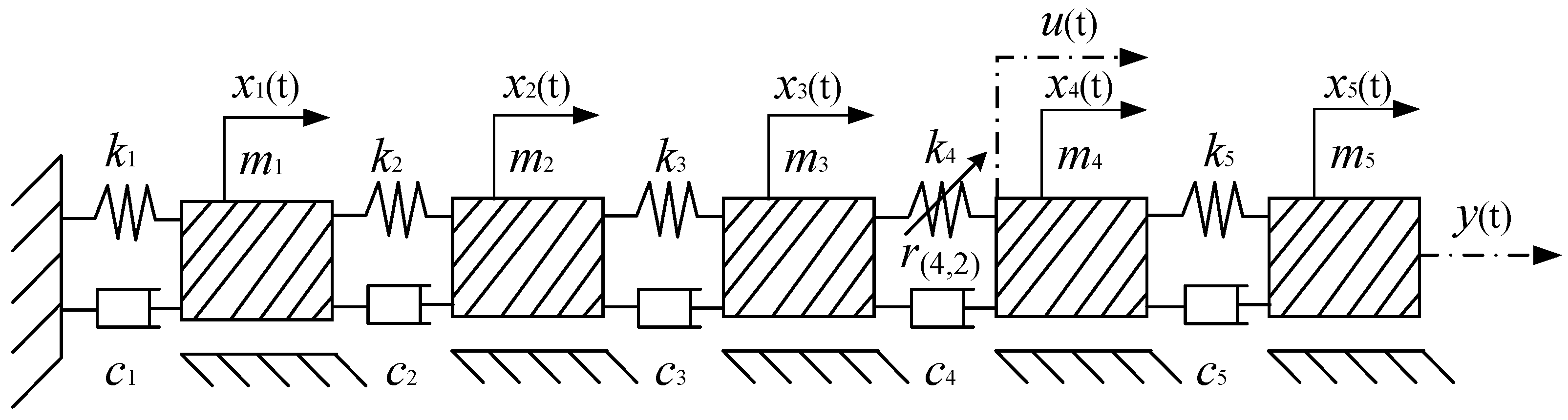
3.1. Dynamic Modeling of One-Dimensional Multi-Degree-of-Freedom Systems
3.2. Structural Damage Detection of MDOF Systems with a Single Nonlinear Spring
- Step 1: Exposure to systematic excitation:
- Step 2: Identification of the NARX model:
- Step 3: Model validation:
- A.
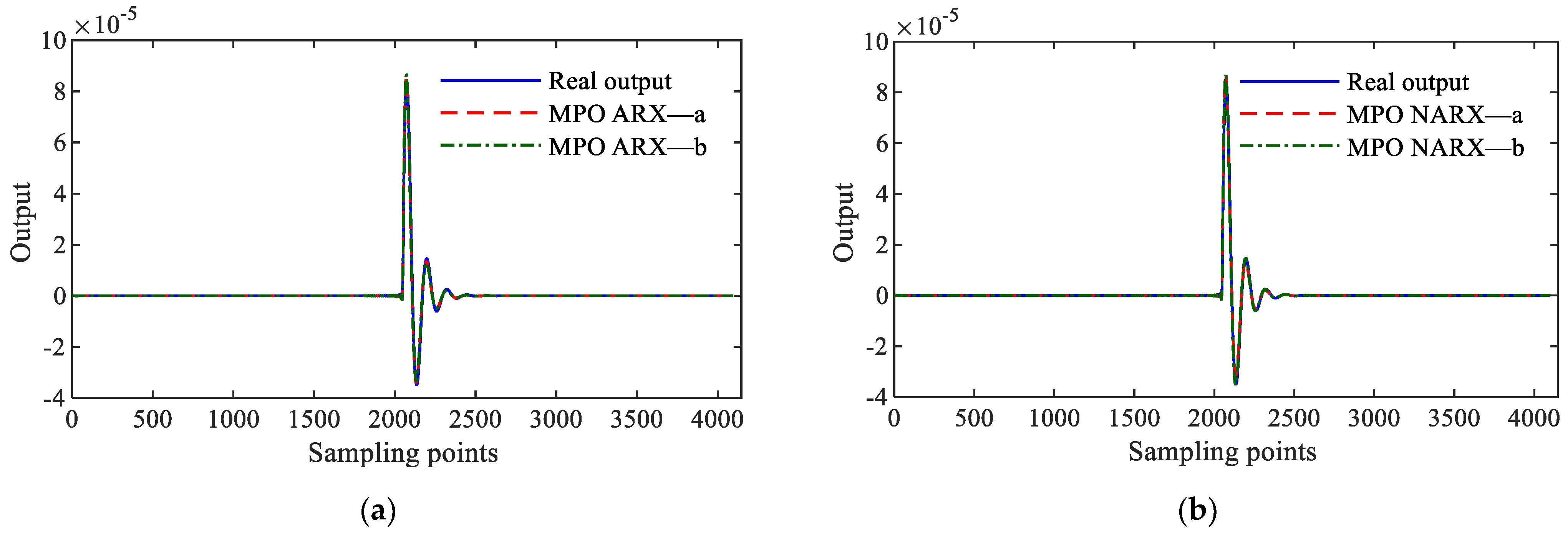
- The validity of the discriminative model is verified using the MPO prediction validation method described in Section 2.2. Figure 4 presents the MPO predictions for the ARX and NARX models of the discriminative MDOF system (16) under shock excitations.
- B.
- The validity of the discriminative model is verified using the MPO prediction validation method described in Section 2.2. Figure 4b illustrates the MPO predictions for the NARX-a and NARX-b models of the discriminative nonlinear MDOF system (23) under various excitations.
- Step 4: Calculate GALEs for the NARX model:
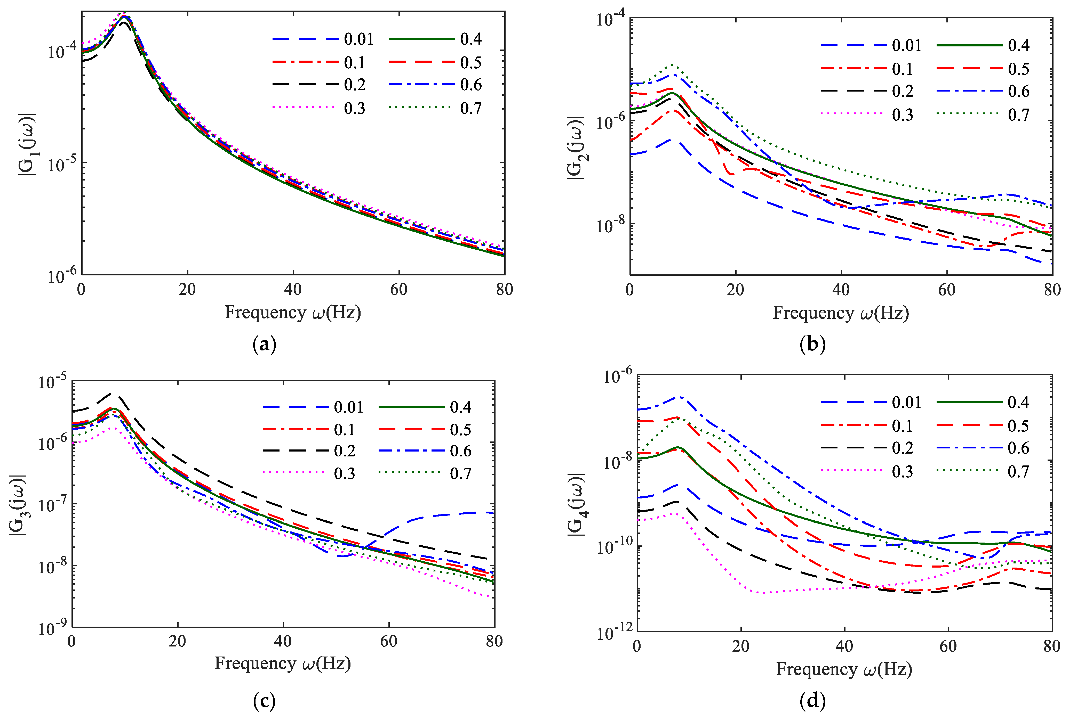
- Step 5: Calculate the NOFRFs of the system:
- Step 6: System condition assessment:
4. Experimental Research
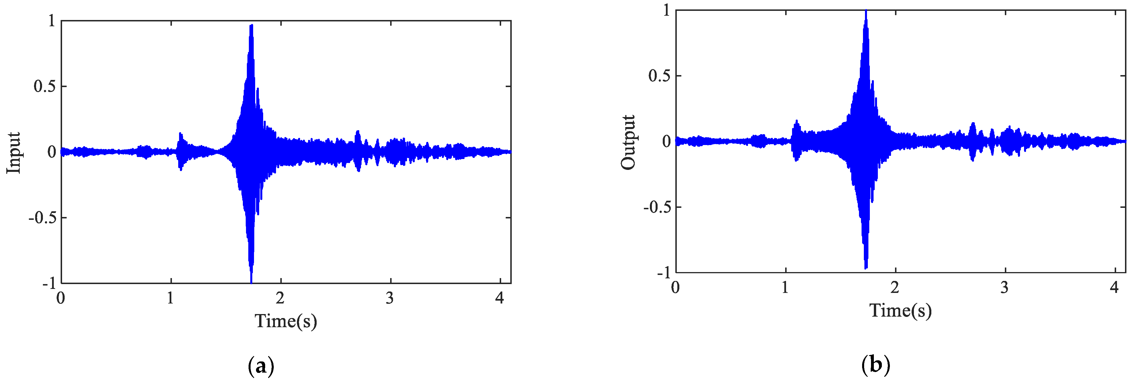
- Step 1: Controlled swept-sine excitation for system identification:
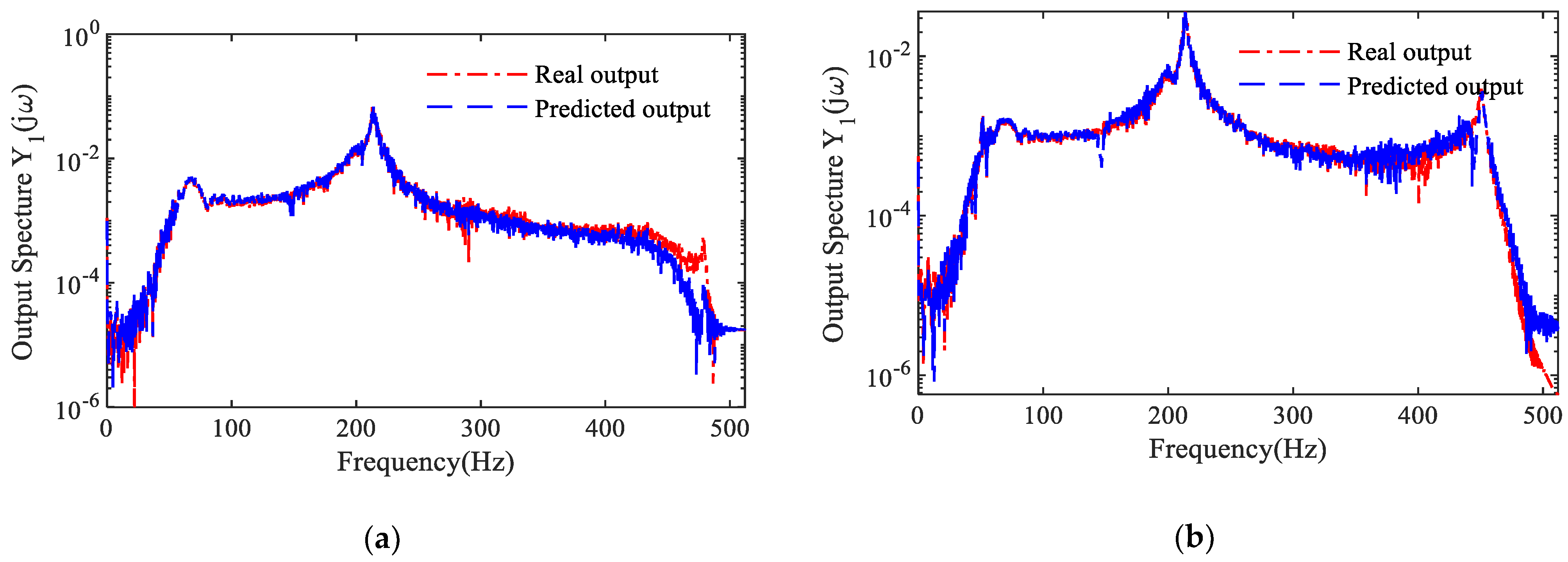
- Step 2: Model validation:
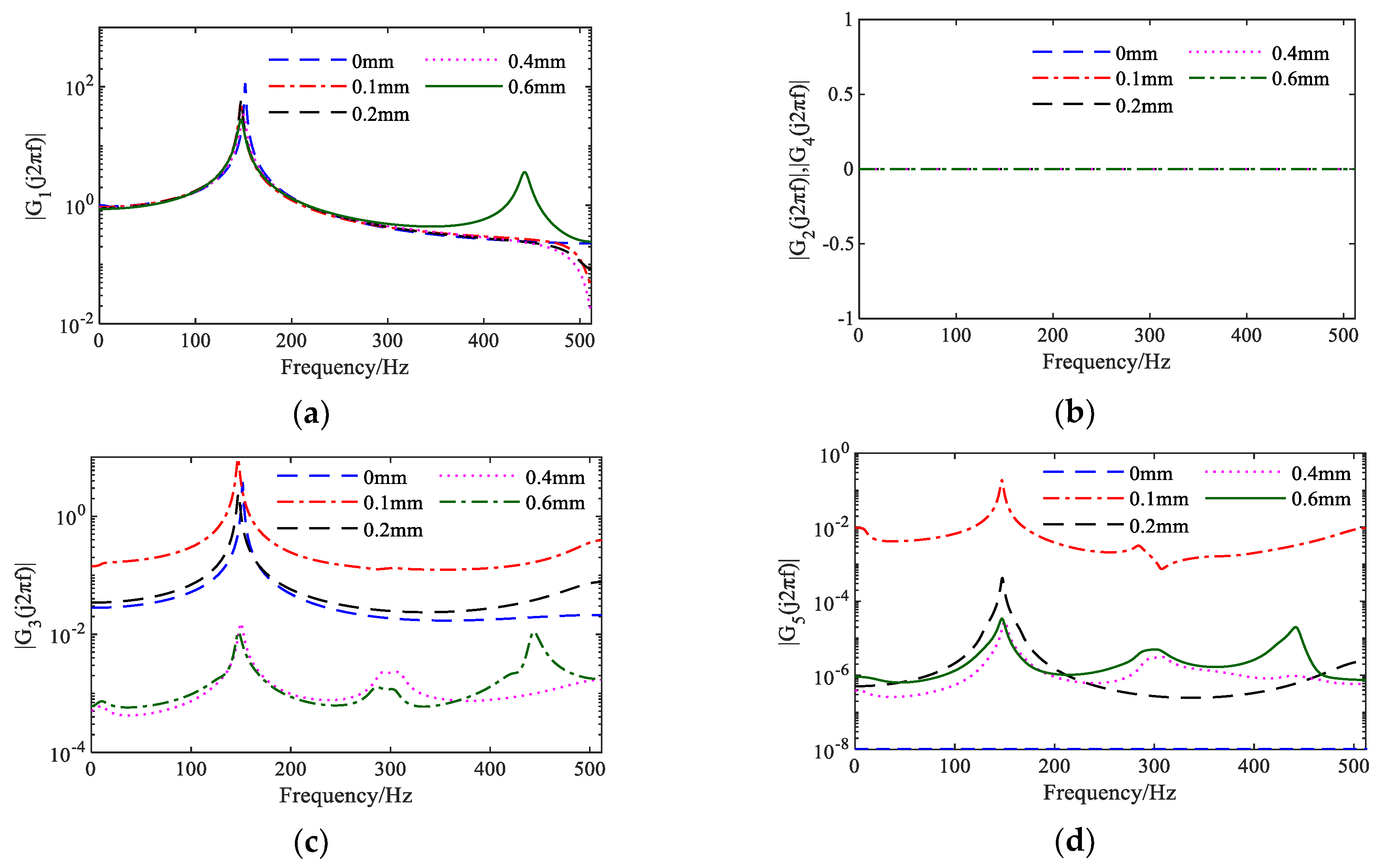
- Step 3: Calculate the NOFRFs of the NARX model:
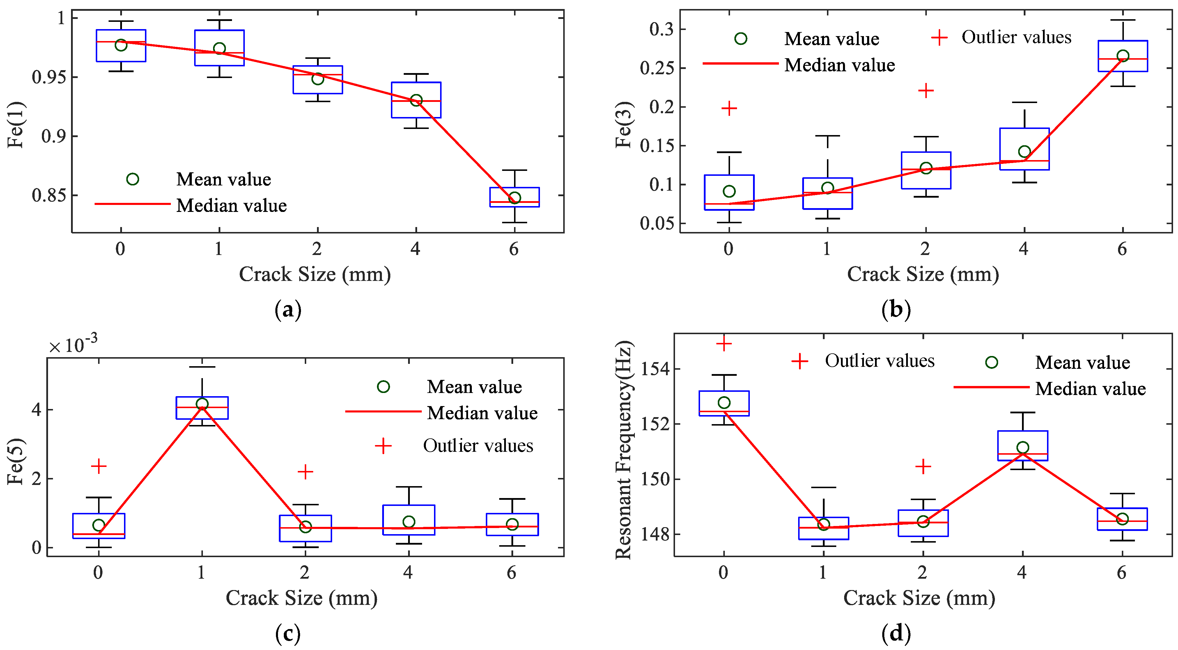
- Step 4: System condition evaluation:
5. Conclusions
Author Contributions
Funding
Institutional Review Board Statement
Informed Consent Statement
Data Availability Statement
Conflicts of Interest
Appendix A
References
- Chen, J.; Yuan, S.; Jin, X. On-line prognosis of fatigue cracking via a regularized particle filter and guided wave monitoring. Mech. Syst. Signal Process. 2019, 131, 1–17. [Google Scholar] [CrossRef]
- Taylor, S.G. Incipient crack detection in a composite wind turbine rotor blade. J. Intell. Mater. Syst. Struct. 2013, 25, 613–620. [Google Scholar] [CrossRef]
- Wang, D.H.; Liao, W.H. Wireless transmission for health monitoring of large structures. IEEE Trans. Instrum. Meas. 2006, 55, 972–981. [Google Scholar] [CrossRef]
- Shan, Q.; Dewhurst, R. Surface-breaking fatigue crack detection using laser ultrasound. Appl. Phys. Lett. 1993, 62, 2649–2651. [Google Scholar] [CrossRef]
- Farrar, C.R.; Doebling, S.W. Damage Detection and Evaluation II. In Modal Analysis and Testing, 2nd ed.; Silva, J.M.M., Maia, N.M.M., Eds.; Springer: Berlin, Germany, 1999; Volume 363, pp. 345–378. [Google Scholar]
- Chen, H.L.; Spyrakos, C.C.; Venkatesh, G. Evaluating structural deterioration by dynamic response. J. Struct. Eng. 1995, 121, 1197–1204. [Google Scholar] [CrossRef]
- Gaetan, K.; Worden, K.; Vakakis, A.F. Past, present and future of nonlinear system identification in structural dynamics. Mech. Syst. Signal Process. 2006, 20, 505–592. [Google Scholar]
- Tsyfansky, S.; Beresnevich, V. Detection of fatigue cracks in flexible geometrically non-linear bars by vibration monitoring. J. Sound Vib. 1998, 213, 159–168. [Google Scholar] [CrossRef]
- Somnay, R.; Ibrahim, R.A.; Banasik, R.C. Nonlinear dynamics of a sliding beam on two supports and its efficacy as a non-traditional isolator. J. Vib. Control 2006, 12, 685–712. [Google Scholar] [CrossRef]
- Peng, Z.K.; Lang, Z.Q.; Wolters, C.; Billings, S.A.; Worden, K. Feasibility study of structural damage detection using NARMAX modelling and Nonlinear Output Frequency Response Function based analysis. Mech. Syst. Signal Process. 2011, 25, 1045–1061. [Google Scholar] [CrossRef]
- Bayma, R.S.; Zhu, Y.P.; Lang, Z.Q. The analysis of nonlinear systems in the frequency domain using Nonlinear Output Frequency Response Functions. Automatica 2018, 94, 452–457. [Google Scholar] [CrossRef]
- Thenozhi, S.; Tang, Y. Nonlinear frequency response based adaptive vibration controller design for a class of nonlinear systems. Mech. Syst. Signal Process. 2018, 99, 930–945. [Google Scholar] [CrossRef]
- Lang, Z.Q.; Billings, S.A. Energy transfer properties of non-linear systems in the frequency domain. Int. J. Control 2005, 78, 345–362. [Google Scholar] [CrossRef]
- Peng, Z.K.; Lang, Z.Q.; Chu, F.L. Numerical analysis of cracked beams using nonlinear output frequency response functions. Comput. Struct. 2008, 86, 1809–1818. [Google Scholar] [CrossRef]
- Zhu, Y.P.; Lang, Z.Q.; Mao, H.L.; Laalej, H. Nonlinear output frequency response functions: A new evaluation approach and applications to railway and manufacturing systems’ condition monitoring. Mech. Syst. Signal Process. 2022, 163, 108179. [Google Scholar] [CrossRef]
- Billings, S.A.; Peyton Jones, J.C. Recursive algorithm for computing the frequency response of a class of non-linear difference equation models. Int. J. Control 1989, 50, 1925–1940. [Google Scholar]
- Chen, S.; Xia, H.; Harris, C.J.; Sharkey, P.M. Sparse mzodeling using orthogonal forward regression with PRESS statistic and regularization. IEEE Trans. Syst. Man Cybern. Part B Cybern. 2004, 34, 898–911. [Google Scholar] [CrossRef]
- Liu, Z.P.; Lang, Z.Q.; Zhu, Y.P.; Gui, Y.; Laalej, H.; Stammers, J. Sensor Data Modeling and Model Frequency Analysis for Detecting Cutting Tool Anomalies in Machining. IEEE Trans. Syst. Man Cybern. Syst. 2023, 53, 2641–2653. [Google Scholar] [CrossRef]
- Bonin, M.; Seghezza, V.; Piroddi, L. NARX model selection based on simulation error minimisation and LASSO. IET Control. Theory Appl. 2010, 4, 1157–1168. [Google Scholar] [CrossRef]
- Efron, B.; Hastie, T.; Johnstone, I.; Tibshirani, R. Least angle regression. Ann. Stat. 2004, 32, 407–451. [Google Scholar] [CrossRef]
- Billings, S.A.; Luo, W. Identification of nonlinear systems using NARX models and forward regression orthogonal least squares (FROLS). Int. J. Control. 2009, 82, 2231–2243. [Google Scholar]
- Zhu, Y.P.; Liu, Z.P.; Zhang, W.B.; Zhang, B. Fast Evaluation of Generalized Associated Linear Equations (GALEs) for Nonlinear Systems Characterization and Compensation. J. Frankl. Inst. 2024, 361, 944–957. [Google Scholar] [CrossRef]
- Zhang, B.; Zhang, W.B.; Peng, Z.K. An analytical study of generalized associated linear equations for a class of nonlinear systems. Chin. J. Theor. Appl. Mech. 2024, 56, 832–846. [Google Scholar]


| Signal Type | Single Harmonic Excitation | Shock Excitation |
|---|---|---|
| ARX-a | 99.81% | 98.92% |
| ARX-b | 99.95% | 99.23% |
| NARX-a | 99.64% | 99.30% |
| NARX-b | 99.57% | 99.37% |
| VAF | 0 mm | 1 mm | 2 mm | 4 mm | 6 mm |
|---|---|---|---|---|---|
| NARX-1 | 99.75% | 99.02% | 99.69% | 99.52% | 99.19% |
| NARX-2 | 99.78% | 98.57% | 99.64% | 94.52% | 99.17% |
Disclaimer/Publisher’s Note: The statements, opinions and data contained in all publications are solely those of the individual author(s) and contributor(s) and not of MDPI and/or the editor(s). MDPI and/or the editor(s) disclaim responsibility for any injury to people or property resulting from any ideas, methods, instructions or products referred to in the content. |
© 2025 by the authors. Licensee MDPI, Basel, Switzerland. This article is an open access article distributed under the terms and conditions of the Creative Commons Attribution (CC BY) license (https://creativecommons.org/licenses/by/4.0/).
Share and Cite
Zhang, W.; Guo, X.; Cheng, L.; Zhang, B. Damage Detection in Beam Structures Based on Frequency-Domain Analysis Methods for Nonlinear Systems. Sensors 2025, 25, 2901. https://doi.org/10.3390/s25092901
Zhang W, Guo X, Cheng L, Zhang B. Damage Detection in Beam Structures Based on Frequency-Domain Analysis Methods for Nonlinear Systems. Sensors. 2025; 25(9):2901. https://doi.org/10.3390/s25092901
Chicago/Turabian StyleZhang, Wenbo, Xiaoyue Guo, Liangliang Cheng, and Bo Zhang. 2025. "Damage Detection in Beam Structures Based on Frequency-Domain Analysis Methods for Nonlinear Systems" Sensors 25, no. 9: 2901. https://doi.org/10.3390/s25092901
APA StyleZhang, W., Guo, X., Cheng, L., & Zhang, B. (2025). Damage Detection in Beam Structures Based on Frequency-Domain Analysis Methods for Nonlinear Systems. Sensors, 25(9), 2901. https://doi.org/10.3390/s25092901