
Extending the Traceability of Dynamic Calibration to the High-Pressure Regime Using a Shock Tube


Abstract
1. Introduction
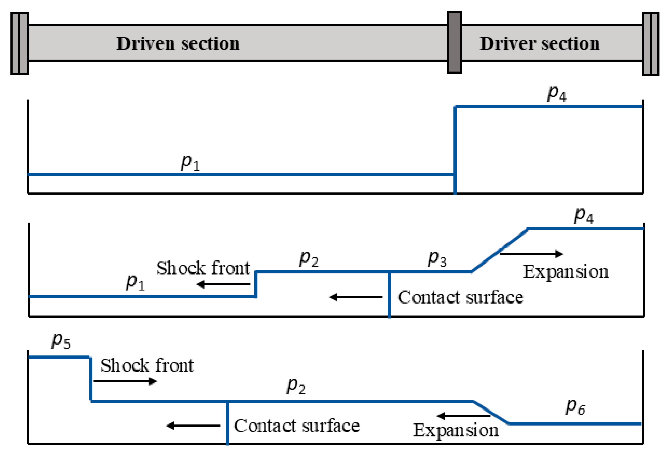
2. Shock Tube Theory
3. Experimental Setup and Procedures
3.1. The Conventional Shock Tube
3.2. The Shock Tube with a Converging Cone
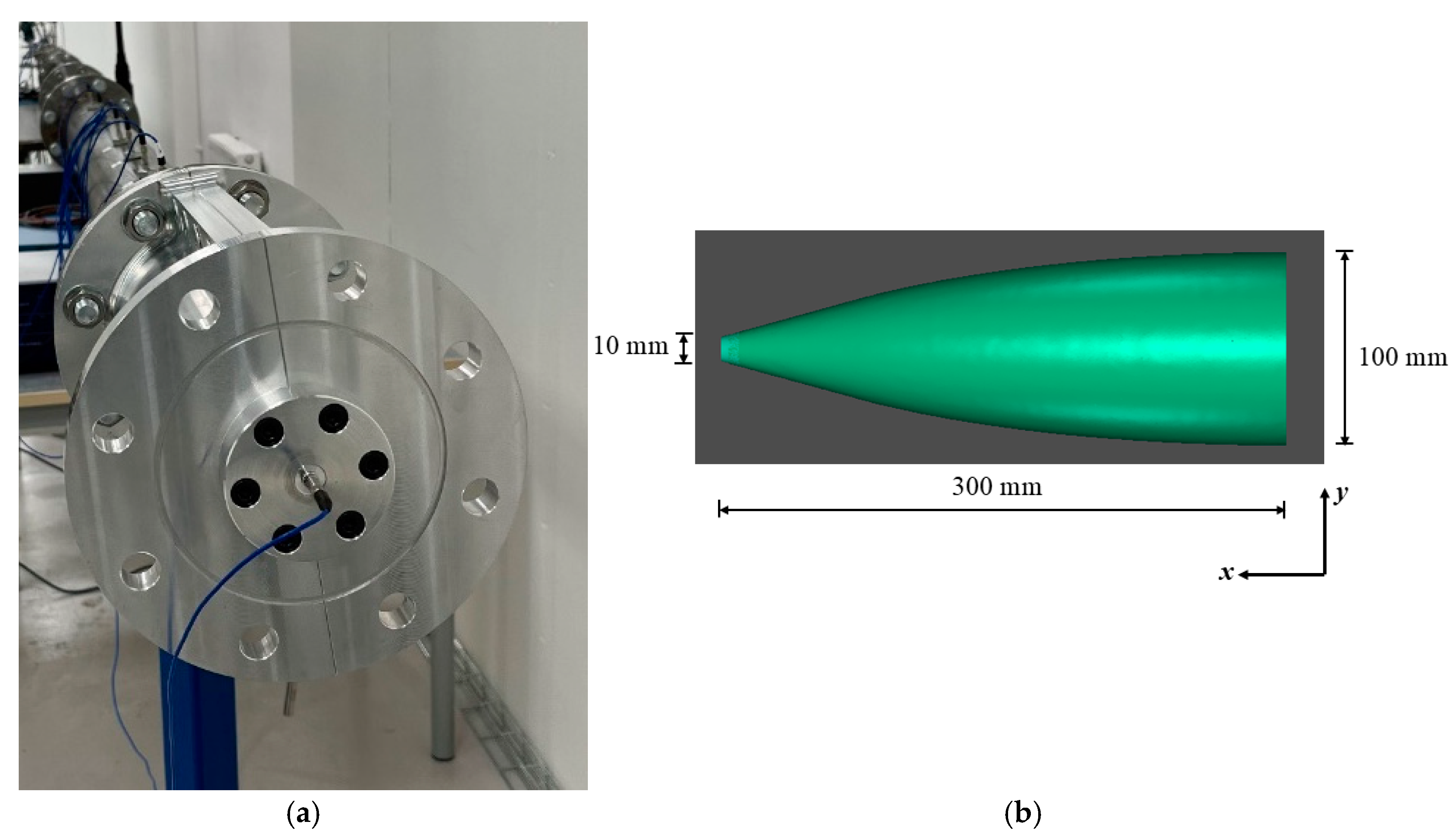
3.2.1. The Configuration of the Converging Cone
3.2.2. Reference Pressure Calculation for the Converging Cone Configuration
3.3. The Shock Tube with an Amplification System
3.3.1. The Design of the Amplification System
3.3.2. Reference Pressure Calculation
3.4. Dynamic Response Calculations
4. Results
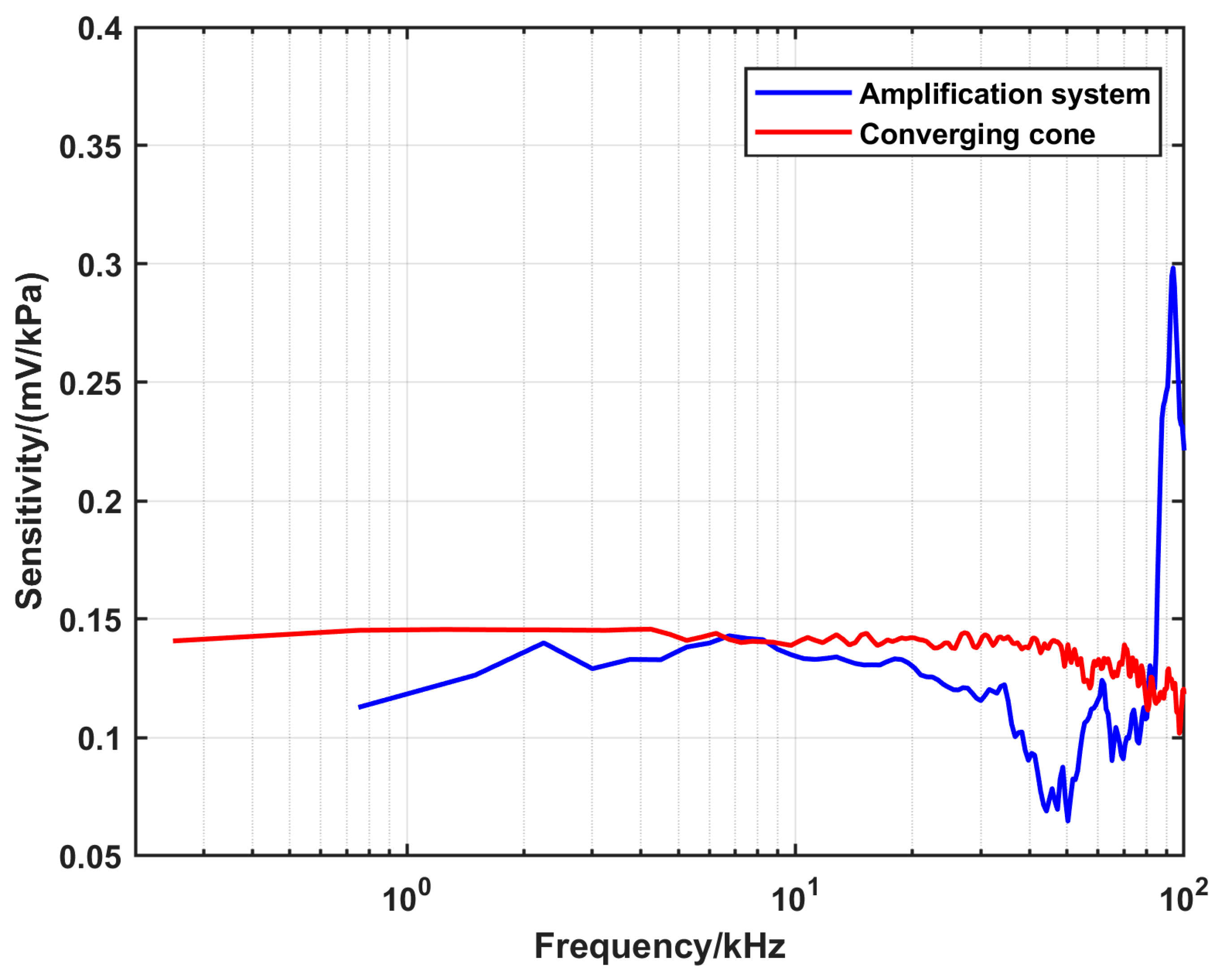
4.1. Characterization of the DUT
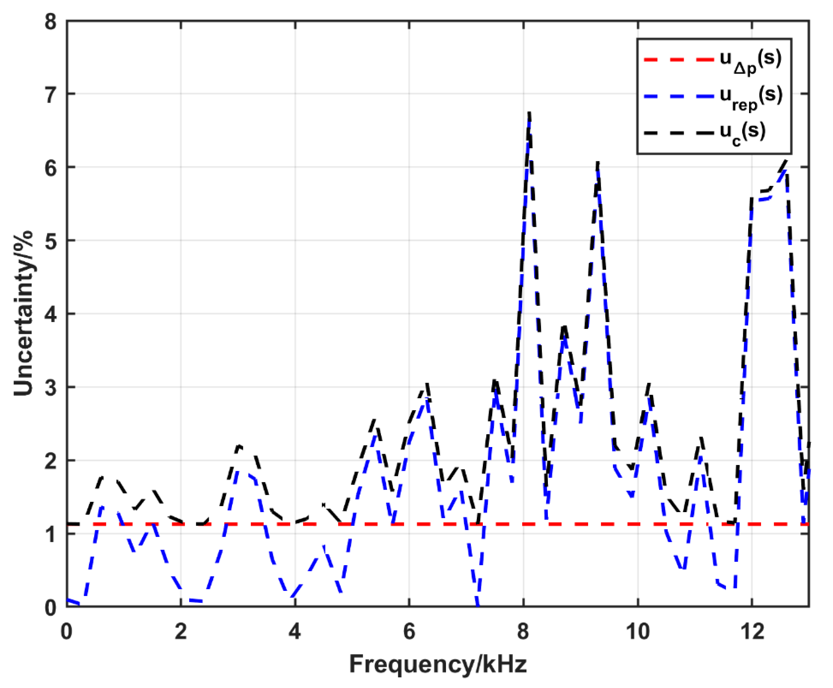
4.2. Uncertainty in Sensitivity Calculations Using the Conventional Tube and the Amplification System
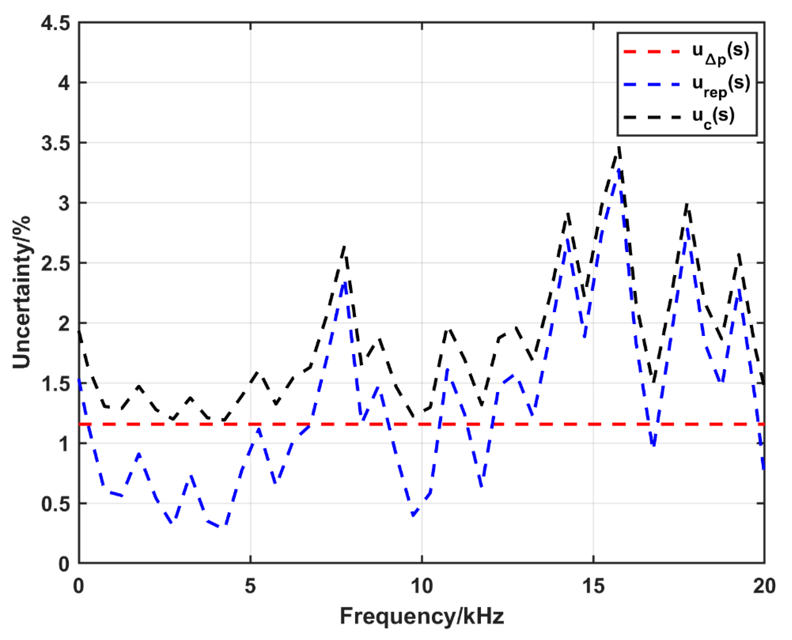
4.3. Uncertainty in Sensitivity in the Case of the Converging Cone
5. Discussion
6. Conclusions
Author Contributions
Funding
Institutional Review Board Statement
Informed Consent Statement
Data Availability Statement
Conflicts of Interest
References
- Broatch, A.; Guardiola, C.; Pla, B.; Bares, P. A direct transform for determining the trapped mass on an internal combustion engine based on the in-cylinder pressure resonance phenomenon. Mech. Syst. Signal Process. 2015, 62–63, 480–489. [Google Scholar] [CrossRef]
- Guardiola, C.; Pla, B.; Bares, P.; Stefanopoulou, A. Cylinder charge composition observation based on in-cylinder pressure measurement. Measurement 2019, 131, 559–568. [Google Scholar] [CrossRef]
- Mohankumar, P.; Ajayan, J.; Yasodharan, R.; Devendran, P.; Sambasivam, R. A review of micromachined sensors for automotive applications. Measurement 2019, 140, 305–322. [Google Scholar] [CrossRef]
- Camussi, R.; Di Marco, A.; Stoica, C.; Bernardini, M.; Stella, F.; De Gregorio, F.; Paglia, F.; Romano, L.; Barbagallo, D. Wind tunnel measurements of the surface pressure fluctuations on the new VEGA-C space launcher. Aerosp. Sci. Technol. 2020, 99, 105772. [Google Scholar] [CrossRef]
- BIPM. The International System of Units (SI), 9th ed.; BIPM: Sevres, France, 2019; ISBN 978-92-822-2272-0. [Google Scholar]
- Salminen, J.; Högström, R.; Saxholm, S.; Lakka, A.; Riski, K.; Heinonen, M. Development of a primary standard for dynamic pressure based on drop weight method covering a range of 10–400 MPa. Metrologia 2018, 55, S52. [Google Scholar] [CrossRef]
- Amer, E.; Jönsson, G.; Arrhén, F. Secondary measurement standard for calibration of dynamic pressure sensor to bridge the gap between existing static and dynamic standards. Measurement 2025, 242, 116253. [Google Scholar] [CrossRef]
- ISA-37. 16.01-2002; A Guide for Dynamic Calibration of Pressure Transducers. The Instrumentation, Systems, and Automation Society: Research Triangle Park, NC, USA, 2002. [Google Scholar]
- Slanina, O.; Quabis, S.; Derksen, S.; Herbst, J.; Wynands, R. Comparing the adiabatic and isothermal pressure dependence of the index of refraction in a drop-weight apparatus. Appl. Phys. B 2020, 126, 175. [Google Scholar] [CrossRef]
- Amer, E.; Jönsson, G.; Arrhén, F. Towards traceable dynamic pressure calibration using a shock tube with an optical probe for accurate phase determination. Metrologia 2022, 59, 035001. [Google Scholar] [CrossRef]
- Amer, E.; Wozniak, M.; Jönsson, G.; Arrhén, F. Evaluation of Shock Tube Retrofitted with Fast-Opening Valve for Dynamic Pressure Calibration. Sensors 2021, 21, 4470. [Google Scholar] [CrossRef] [PubMed]
- Andrej, S.; Jože, K. Characterization of a newly developed diaphragmless shock tube for the primary dynamic calibration of pressure meters. Metrologia 2020, 57, 055009. [Google Scholar]
- Sarraf, C.; Damion, J.-P. Dynamic pressure sensitivity determination with Mach number method. Meas. Sci. Technol. 2018, 29, 054006. [Google Scholar] [CrossRef]
- Sundarapandian, S.; Liverts, M. On using converging shock waves for pressure amplification in shock tubes. Metrologia 2020, 57, 035008. [Google Scholar] [CrossRef]
- Shen, H.-P.S.; Vanderover, J.; Oehlschlaeger, M.A. A shock tube study of the auto-ignition of toluene/air mixtures at high pressures. Proc. Combust. Inst. 2009, 32, 165–172. [Google Scholar] [CrossRef]
- Döntgen, M.; Fuller, M.E.; Peukert, S.; Nativel, D.; Schulz, C.; Alexander Heufer, K.; Franklin Goldsmith, C. Shock tube study of the pyrolysis kinetics of Di- and trimethoxy methane. Combust. Flame 2022, 242, 112186. [Google Scholar] [CrossRef]
- Amadio, A.R.; Crofton, M.W.; Petersen, E.L. Test-time extension behind reflected shock waves using CO2–He and C3H8–He driver mixtures. Shock. Waves 2006, 16, 157–165. [Google Scholar] [CrossRef]
- Campbell, M.F.; Parise, T.; Tulgestke, A.M.; Spearrin, R.M.; Davidson, D.F.; Hanson, R.K. Strategies for obtaining long constant-pressure test times in shock tubes. Shock. Waves 2015, 25, 651–665. [Google Scholar] [CrossRef]
- Oertel, H. Stossrohre; Springer: New York, NY, USA, 1966. [Google Scholar]
- Anderson, J.D. Modern Compressible Flow, 3rd ed.; The Boeing Company: Singapore, 2004. [Google Scholar]
- Kjellander, M.; Tillmark, N.; Apazidis, N. Energy concentration by spherical converging shocks generated in a shock tube. Phys. Fluid 2012, 24, 126103. [Google Scholar] [CrossRef]
- Kjellander, M. Energy Concentration by Converging Shock Waves in Gases. Ph.D. Thesis, Royal Institute of Technology KTH, Stockholm, Sweden, 2012. [Google Scholar]
- OpenFOAM: User Guide. Available online: https://www.openfoam.com/documentation/guides/latest/doc/guide-applications-solvers-compressible-rhoCentralFoam.html (accessed on 9 March 2025).
- Kurganov, A.; Tadmor, E. New High-Resolution Central Schemes for Nonlinear Conservation Laws and Convection–Diffusion Equations. J. Comput. Phys. 2000, 160, 241–282. [Google Scholar] [CrossRef]
- Oakley, J.G.; Bonazza, R. xt.exe Software; Wisconsin Shock Tube Laboratory: Madison, WI, USA, 2004. [Google Scholar]
- Hjelmgren, J. “Dynamic Measurement of Pressure—A Literature Survey” SP Report; SP Swedish National Testing and Research Institute: Borås, Sweden, 2002. [Google Scholar]
- JCGM 100:2008; Evaluation of Measurement Data—Guide to the Expression of Uncertainty in Measurement. Joint Committee for Guides in Metrology: Paris, France, 2008.


| Driven Section | Driver Section | ||||
|---|---|---|---|---|---|
| IC | BC Walls | IC | BC Walls | BC Inlet | |
| P (kPa) | 100 | zeroGradient | Calculated [25] | zeroGradient | waveTransmissive uniform calculated [25] |
| U (m/s) | 0 | fixedValue (0, 0, 0) | Calculated [25] | fixedValue (0, 0, 0) | zeroGradient |
| T (K) | 294.15 | fixedValue 294.15 | Calculated [25] | fixedValue calculated [25] | zeroGradient |
| Configuration | Conventional | Converging Cone | Amplification System (First Trial) | Amplification System |
|---|---|---|---|---|
| Reference pressure profile | Step-like | Blast | Blast | Step-like |
| Reference pressure amplitude (MPa) | 0.1–1.5 | 5–25 | 3–12 | 1–7 |
| Constant pressure time (ms) | 2–3 | ≤0.005 | 0.02 | 0.2–0.3 |
| Calculation of the reference pressure | Analytical solution | Numerical simulation | Numerical simulation | Analytical solution |
| Driven Gas | Driver Gas | p1 (kPa) | p4 (kPa) | Δp (MPa) | Average Sensitivity (mV/kPa) | |
|---|---|---|---|---|---|---|
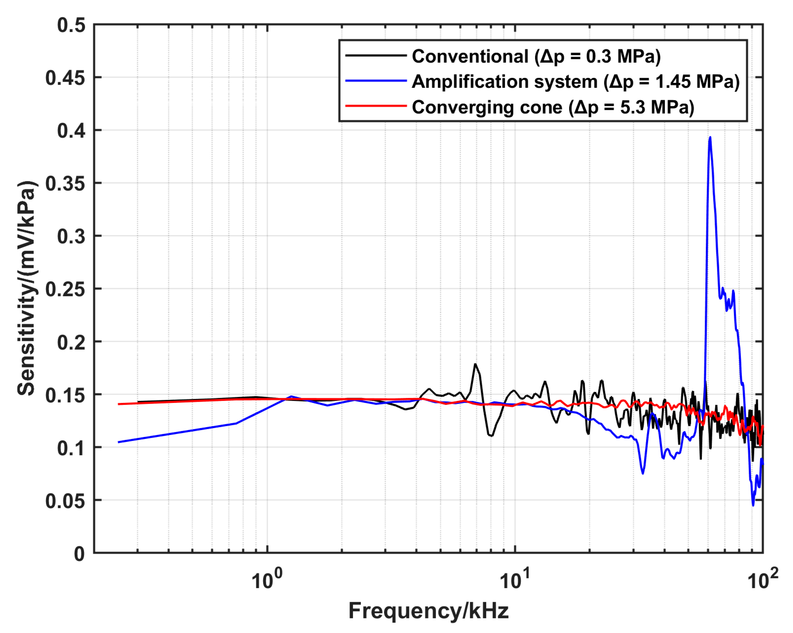
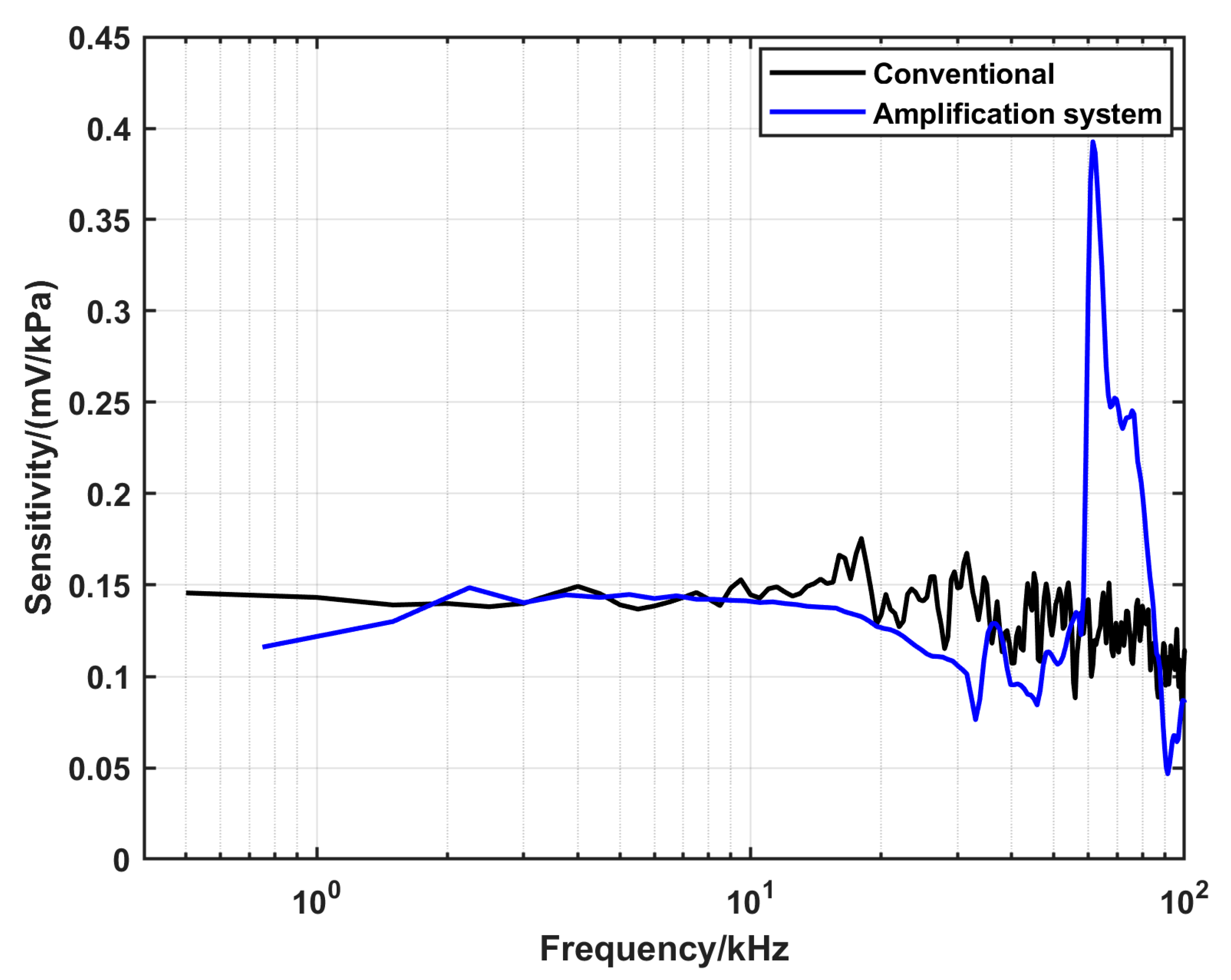
| Conventional | Ar | Ar | 100 | 800 | 0.30 | 0.145 (up to 20 kHz) |
| Amplification system | Ar | Ar | 100 | 800 | 1.45 | 0.142 (from 2 kHz to 13 kHz) |
| Converging cone | Ar | Ar | 100 | 800 | 5.30 | 0.142 (up to 20 kHz) |
| Parameter | Standard Uncertainty, k = 1 | Distribution |
| Temperature (K) | 0.6 | Normal |
| Time (s) | 0.4 × 10⁻⁶ (conventional) 2.5 × 10⁻⁶ (amplification system) | Normal |
| Side-wall sensors positions (m) | 10−4 | Normal |
| Specific heat ratio γ1 | 10−4 | Normal |
| Initial driven pressure p1 (Pa) | 100 | Normal |
| The Input Parameters | The Standard Uncertainty in the Input Parameters (k = 1) | The Corresponding Standard Uncertainty in p5 (k = 1) (kPa) |
|---|---|---|
| P2 (kPa) | 0.6 | 18.2 |
| U2 (m/s) | 0.4 | 11.0 |
| T2 (K) | 0.5 | 0.1 |
| Cone dimensions (m) | 5 × 10⁻⁵ | 0.4% of p5 (22 kPa) |
Disclaimer/Publisher’s Note: The statements, opinions and data contained in all publications are solely those of the individual author(s) and contributor(s) and not of MDPI and/or the editor(s). MDPI and/or the editor(s) disclaim responsibility for any injury to people or property resulting from any ideas, methods, instructions or products referred to in the content. |
© 2025 by the authors. Licensee MDPI, Basel, Switzerland. This article is an open access article distributed under the terms and conditions of the Creative Commons Attribution (CC BY) license (https://creativecommons.org/licenses/by/4.0/).
Share and Cite
Amer, E.; Jönsson, G.; Penttinen, O.; Arrhén, F. Extending the Traceability of Dynamic Calibration to the High-Pressure Regime Using a Shock Tube. Sensors 2025, 25, 2453. https://doi.org/10.3390/s25082453
Amer E, Jönsson G, Penttinen O, Arrhén F. Extending the Traceability of Dynamic Calibration to the High-Pressure Regime Using a Shock Tube. Sensors. 2025; 25(8):2453. https://doi.org/10.3390/s25082453
Chicago/Turabian StyleAmer, Eynas, Gustav Jönsson, Olle Penttinen, and Fredrik Arrhén. 2025. "Extending the Traceability of Dynamic Calibration to the High-Pressure Regime Using a Shock Tube" Sensors 25, no. 8: 2453. https://doi.org/10.3390/s25082453
APA StyleAmer, E., Jönsson, G., Penttinen, O., & Arrhén, F. (2025). Extending the Traceability of Dynamic Calibration to the High-Pressure Regime Using a Shock Tube. Sensors, 25(8), 2453. https://doi.org/10.3390/s25082453