
Identification of Defects in Low-Speed and Heavy-Load Mechanical Systems Using Multi-Fusion Analytic Mode Decomposition Method


Abstract
1. Introduction
2. Theoretical Descriptions
- (1)
- Synchronously collect multi-channel signals.
- (2)
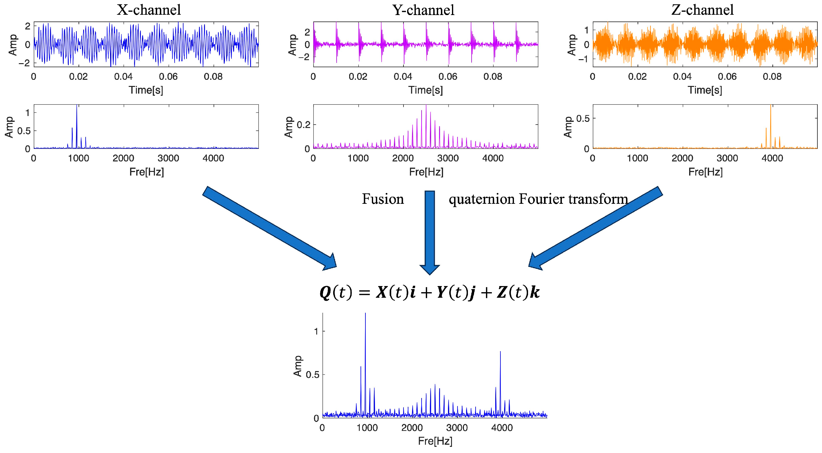
- Use quaternion theory to fuse multiple channels or multiple groups of signals into quaternion signals.
- (3)
- Calculate the spectrum of multiple groups or multi-channel signals after fusion in the frequency domain.
- (4)
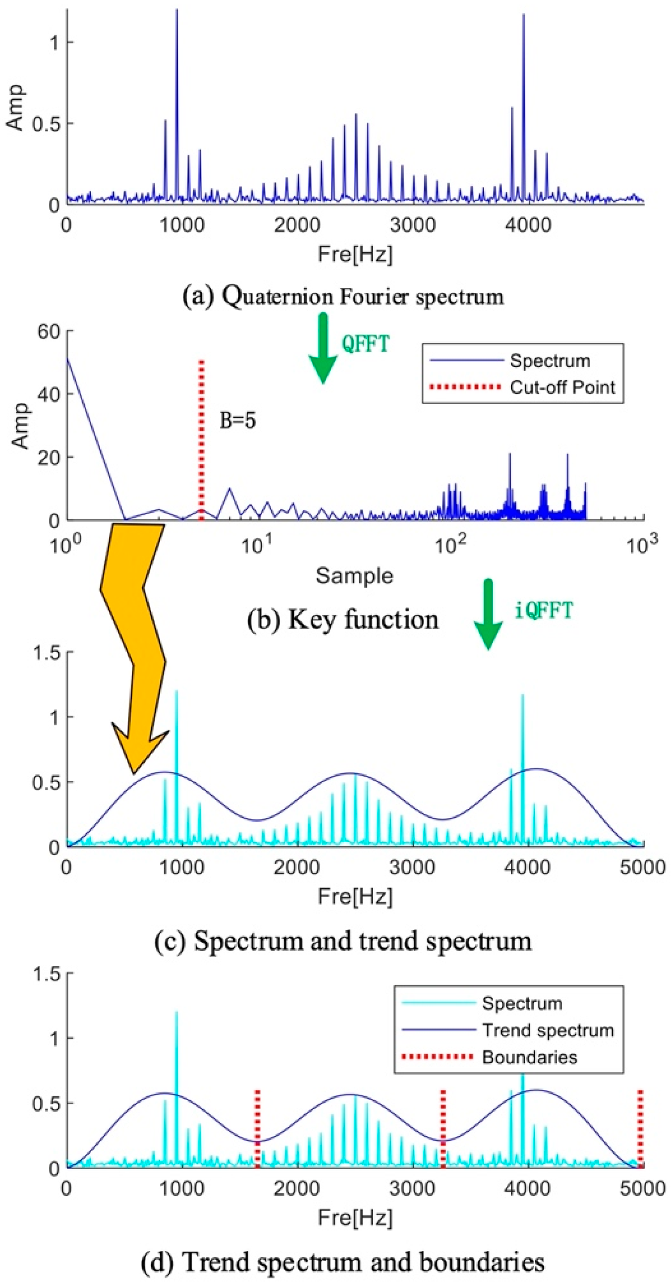
- Acquire the trend spectrum and apply the Fourier transform to the fused spectrum.
- (5)
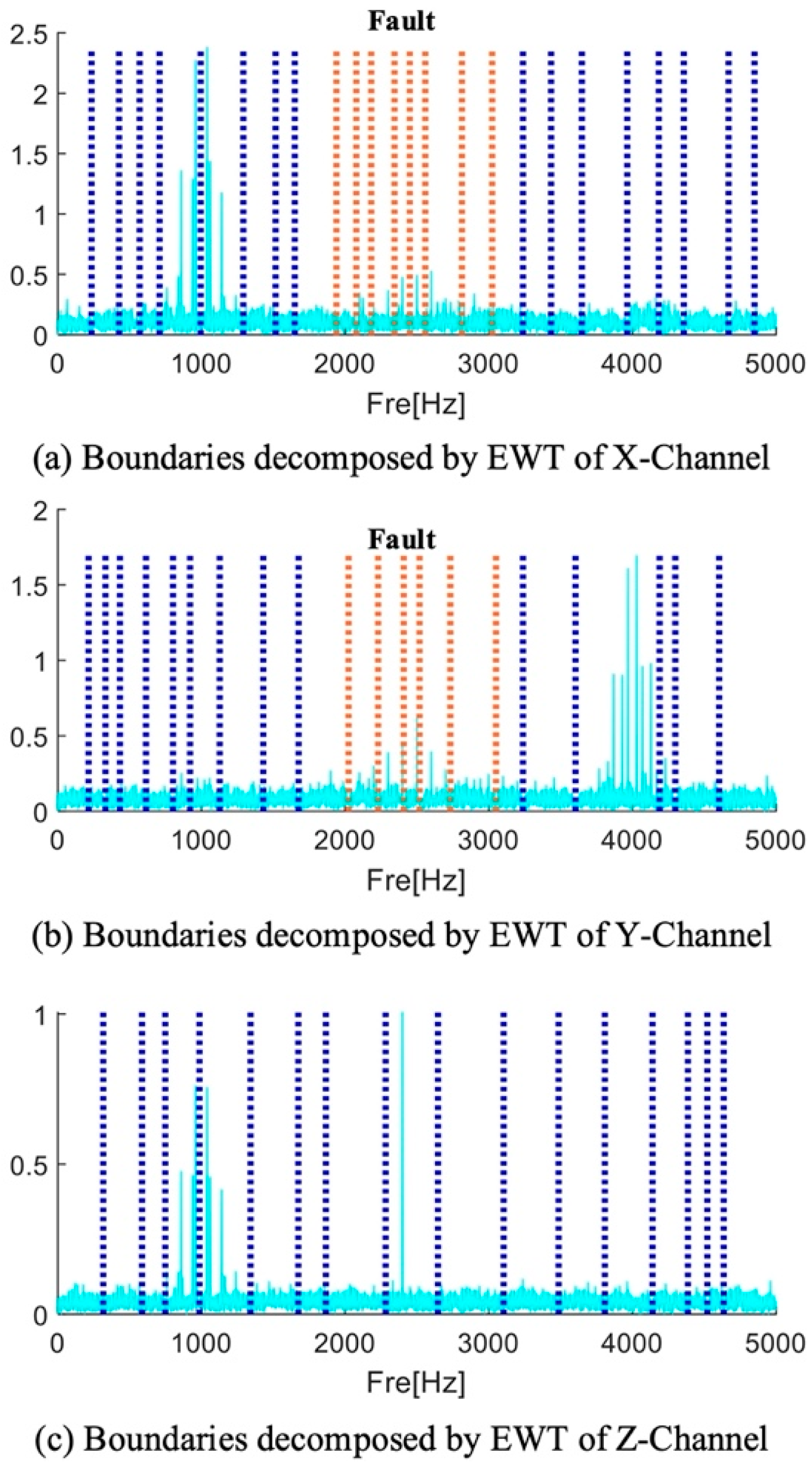
- Obtain multiple frequency band components and split the fused spectrum into frequency bands using the trend spectrum.
- (6)
- Perform model decomposition iteratively to obtain several components.
2.1. Multi-Signal Frequency Domain Fusion Method
2.2. Spectrum Segmentation Method Based on Multi-Signal Frequency Domain Fusion
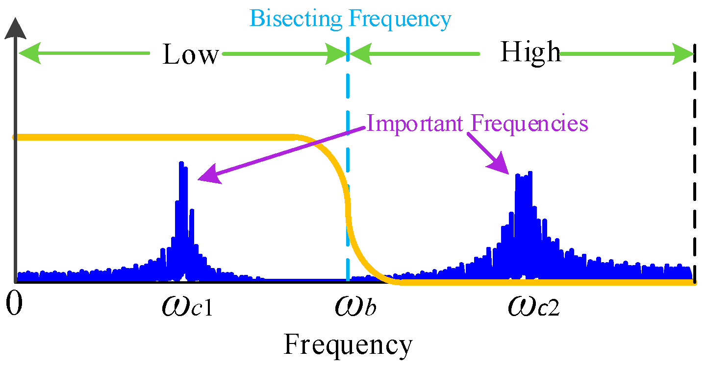
2.3. Multi-Fusion Analytic Mode Decomposition
3. Simulation Verification Analysis
4. Experimental Analysis
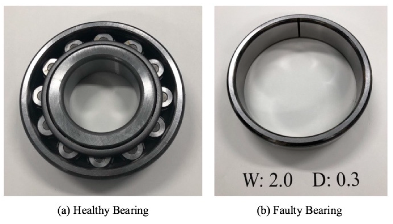
4.1. Bearing Outer Ring
4.2. Bearing Inner Ring
5. Conclusions
Author Contributions
Funding
Institutional Review Board Statement
Informed Consent Statement
Data Availability Statement
Conflicts of Interest
References
- Tang, H.; Liao, Z.; Chen, P.; Zuo, D.; Yi, S. Robust Deep Learning Network for Low-speed Machinery Fault Diagnosis based on Multi-kernel and RPCA. IEEE Trans. Mechatron. 2021, 27, 1522–1532. [Google Scholar] [CrossRef]
- Huo, W.; Jiang, Z.; Sheng, Z.; Zhang, K.; Xu, Y. Cyclostationarity blind deconvolution via eigenvector screening and its applications to the condition monitoring of rotating machinery. Mech. Syst. Signal Process. 2025, 222, 111782. [Google Scholar] [CrossRef]
- Zhang, K.; Liu, Y.; Zhang, L.; Ma, C.; Xu, Y. Frequency slice graph spectrum model and its application in bearing fault feature extraction. Mech. Syst. Signal Process. 2025, 226, 112383. [Google Scholar] [CrossRef]
- Chen, T.; Guo, L.; Feng, T.; Gao, H.; Yu, Y. IESMGCFFOgram: A new method for multicomponent vibration signal demodulation and rolling bearing fault diagnosis. Mech. Syst. Signal Process. 2023, 204, 110800. [Google Scholar] [CrossRef]
- Ma, C.; Zhang, W.; Shi, M.; Zou, X.; Xu, Y.; Zhang, K. Feature identification based on cepstrum-assisted frequency slice function for bearing fault diagnosis. Measurement 2025, 246, 116753. [Google Scholar] [CrossRef]
- Wang, H.; Yan, C.; Liu, Y.; Li, S.; Meng, J. The LFIgram: A Targeted Method of Optimal Demodulation Band Selection for Compound Faults Diagnosis of Rolling Bearing. IEEE Sens. J. 2024, 24, 6687–6699. [Google Scholar] [CrossRef]
- Glowacz, A. Acoustic based fault diagnosis of three-phase induction motor. Appl. Acoust. 2018, 137, 82–89. [Google Scholar] [CrossRef]
- Glowacz, A.; Glowacz, Z. Diagnosis of stator faults of the single-phase induction motor using acoustic signals. Appl. Acoust. 2017, 117, 20–27. [Google Scholar] [CrossRef]
- Lu, W.; Jiang, W.; Wu, H.; Hou, J. A fault diagnosis scheme of rolling element bearing based on near-field acoustic holography and gray level co-occurrence matrix. J. Sound Vib. 2012, 331, 3663–3674. [Google Scholar] [CrossRef]
- Hu, Y.; Tu, X.; Li, F.; Li, H.; Meng, G. An adaptive and tacholess order analysis method based on enhanced empirical wavelet transform for fault detection of bearings with varying speeds. J. Sound Vib. 2017, 409, 241–255. [Google Scholar] [CrossRef]
- Zhang, K.; Xu, Y.; Liao, Z.; Song, L.; Chen, P. A novel Fast Entrogram and its applications in rolling bearing fault diagnosis. Mech. Syst. Signal Process. 2021, 154, 107582. [Google Scholar] [CrossRef]
- Kumar, A.; Gandhi, C.; Zhou, Y.; Kumar, R.; Xiang, J. Variational mode decomposition based symmetric single valued neutrosophic cross entropy measure for the identification of bearing defects in a centrifugal pump. Appl. Acoust. 2020, 165, 107294. [Google Scholar] [CrossRef]
- Tao, Y.; Ge, C.; Feng, H.; Xue, H.; Yao, M.; Tang, H.; Liao, Z.; Chen, P. A novel approach for adaptively separating and extracting compound fault features of the in-wheel motor bearing. ISA Trans. 2025, in press. [CrossRef]
- Feng, H.; Tao, Y.; Feng, J.; Zhang, Y.; Xue, H.; Wang, T.; Xu, X.; Chen, P. Fault-Tolerant Collaborative Control of Four-Wheel-Drive Electric Vehicle for One or More In-Wheel Motors’ Faults. Sensors 2025, 25, 1540. [Google Scholar] [CrossRef]
- Chen, J.; Li, Z.; Pan, J.; Chen, G.; Zi, Y.; Yuan, J.; Chen, B.; He, Z. Wavelet transform based on inner product in fault diagnosis of rotating machinery: A review. Mech. Syst. Signal Process. 2016, 70–71, 1–35. [Google Scholar] [CrossRef]
- Lei, Y.; Lin, J.; He, Z.; Zuo, M.J. A review on empirical mode decomposition in fault diagnosis of rotating machinery. Mech. Syst. Signal Process. 2013, 35, 108–126. [Google Scholar] [CrossRef]
- Xue, R.; Wang, X.; Yang, Q.; Dong, F.; Zhang, Y.; Cao, J.; Song, G. Grain size characterization of aluminum based on ensemble empirical mode decomposition using a laser ultrasonic technique. Appl. Acoust. 2019, 156, 378–386. [Google Scholar] [CrossRef]
- Jiang, X.; Song, Q.; Wang, H.; Du, G.; Guo, J.; Shen, C.; Zhu, Z. Central frequency mode decomposition and its applications to the fault diagnosis of rotating machines. Mech. Mach. Theory 2022, 174, 104919. [Google Scholar] [CrossRef]
- Yao, J.; Liu, C.; Song, K.; Feng, C.; Jiang, D. Fault diagnosis of planetary gearbox based on acoustic signals. Appl. Acoust. 2021, 181, 108151. [Google Scholar] [CrossRef]
- Chen, G.; Wang, Z. A signal decomposition theorem with Hilbert transform and its application to narrowband time series with closely spaced frequency components. Mech. Syst. Signal Process. 2012, 28, 258–279. [Google Scholar] [CrossRef]
- Wang, Z.-C.; Ren, W.-X.; Liu, J.-L. A synchrosqueezed wavelet transform enhanced by extended analytical mode decomposition method for dynamic signal reconstruction. J. Sound Vib. 2013, 332, 6016–6028. [Google Scholar] [CrossRef]
- Qu, H.; Li, T.; Chen, G. Multiple analytical mode decompositions (M-AMD) for high accuracy parameter identification of nonlinear oscillators from free vibration. Mech. Syst. Signal Process. 2018, 117, 483–497. [Google Scholar] [CrossRef]
- Qu, H.; Li, T.; Wang, R.; Li, J.; Guan, Z.; Chen, G. Application of adaptive wavelet transform based multiple analytical mode decomposition for damage progression identification of Cable-Stayed bridge via shake table test. Mech. Syst. Signal Process. 2021, 149, 107055. [Google Scholar] [CrossRef]
- Wu, X.; Tian, M.; Zhu, Y.; Zhao, Q.; Liu, F. A time frequency domain digital implementation of flickermeter using analytical mode decomposition. Int. Trans. Electr. Energy Syst. 2019, 29, 12016. [Google Scholar] [CrossRef]
- Qu, Q.; Dong, Y.; Zheng, Y. Recursive Dynamic inner PrincipalComponent Analysis for Adaptive ProcessModeling. IFAC-PapersOnLine 2024, 58, 682–687. [Google Scholar] [CrossRef]
- Zhou, R.; Zhang, Z.; Fu, H.; Zhang, L.; Li, L.; Huang, G.; Li, F.; Yang, X.; Dong, Y.; Zhang, Y.-T.; et al. PR-PL: A Novel Prototypical Representation Based Pairwise Learning Framework for Emotion Recognition Using EEG Signals. IEEE Trans. Affect. Comput. 2023, 15, 657–670. [Google Scholar] [CrossRef]
- Yin, C.; Li, Y.; Wang, Y.; Dong, Y. Physics-guided degradation trajectory modeling for remaining useful life prediction of rolling bearings. Mech. Syst. Signal Process. 2024, 224, 112192. [Google Scholar] [CrossRef]
- Zhang, K.; Xu, Y.; Chen, P. Feature extraction by enhanced analytical mode decomposition based on order statistics filter. Measurement 2021, 173, 108620. [Google Scholar] [CrossRef]
- Wang, Z.-C.; Ge, B.; Ren, W.-X.; Hou, J.; Li, D.; He, W.-Y.; Chen, T. Discrete analytical mode decomposition with automatic bisecting frequency selection for structural dynamic response analysis and modal identification. J. Sound Vib. 2020, 484, 115520. [Google Scholar] [CrossRef]
- Zhao, Y.; Zhang, J.; Zhao, Q. Online Monitoring of Low-Frequency Oscillation Based on the Improved Analytical Modal Decomposition Method. IEEE Access 2020, 8, 215256–215266. [Google Scholar] [CrossRef]
- Bendoumia, R.; Djendi, M. Acoustic noise reduction by new two-channel proportionate forward symmetric adaptive decorrelating algorithms in sparse systems. Appl. Acoust. 2018, 137, 69–81. [Google Scholar] [CrossRef]
- Jeon, O.; Ryu, H.; Kim, H.G.; Wang, S. Vibration localization prediction and optimal exciter placement for improving the sound field op-timization performance of multi-channel distributed mode loudspeakers. J. Sound Vib. 2020, 481, 115424. [Google Scholar] [CrossRef]
- Hamdan, E.C.; Fazi, F.M. A modal analysis of multichannel crosstalk cancellation systems and their relationship to amplitude panning. J. Sound Vib. 2020, 490, 115743. [Google Scholar] [CrossRef]
- Salah, E.; Amine, K.; Redouane, K.; Fares, K. A Fourier transform based audio watermarking algorithm. Appl. Acoust. 2021, 172, 107652. [Google Scholar] [CrossRef]
- Martins, P.V.; Silva, O.M.; Lenzi, A. Insertion loss analysis of slender beams with periodic curvatures using quaternion-based parametrization, FE method and wave propagation approach. J. Sound Vib. 2019, 455, 82–95. [Google Scholar] [CrossRef]
- Jiang, X.; Li, X.; Wang, Q.; Song, Q.; Liu, J.; Zhu, Z. Multi-sensor data fusion-enabled semi-supervised optimal temperature-guided PCL framework for machinery fault diagnosis. Inf. Fusion 2024, 101, 102005. [Google Scholar] [CrossRef]
- Yi, C.; Lv, Y.; Dang, Z.; Xiao, H.; Yu, X. Quaternion singular spectrum analysis using convex optimization and its application to fault diagnosis of rolling bearing. Measurement 2017, 103, 321–332. [Google Scholar] [CrossRef]
- Ma, Y.; Cheng, J.; Hu, N.; Cheng, Z.; Yang, Y. Symplectic quaternion singular mode decomposition with application in gear fault diagnosis. Mech. Mach. Theory 2021, 160, 104266. [Google Scholar] [CrossRef]
- Hamilton, W.R., II. On quaternions; or on a new system of imaginaries in algebra. J. Comput. Educ. 1844, 25, 10–13. [Google Scholar] [CrossRef]
- Ortolani, F.; Comminiello, D.; Scarpiniti, M.; Uncini, A. Frequency domain quaternion adaptive filters: Algorithms and convergence performance. Signal Process. 2017, 136, 69–80. [Google Scholar] [CrossRef]
- Ell, T.A.; Le Bihan, N.; Sangwine, S.J. Quaternion Fourier Transforms for Signal and Image Processing; Wiley: London, UK, 2014. [Google Scholar]
- Sangwine, S.J. The Discrete Quaternion Fourier Transform. In Proceedings of the 1997 Sixth International Conference on Image Processing and Its Applications, Dublin, Ireland, 14–17 July 1997; Volume 2, pp. 790–793. [Google Scholar]
- Ell, T.A.; Sangwine, S.J. Decomposition of 2D hypercomplex Fourier transforms into pairs of complex Fourier transforms. In Proceedings of the 10th European Signal Processing Conference (EUSIPCO), Tampere, Finland, 4–8 September 2000. [Google Scholar]
- Gilles, J. Empirical Wavelet Transform. IEEE Trans. Signal Process. 2013, 61, 3999–4010. [Google Scholar] [CrossRef]
- Antoni, J. Fast computation of the kurtogram for the detection of transient faults. Mech. Syst. Signal Process. 2007, 21, 108–124. [Google Scholar] [CrossRef]


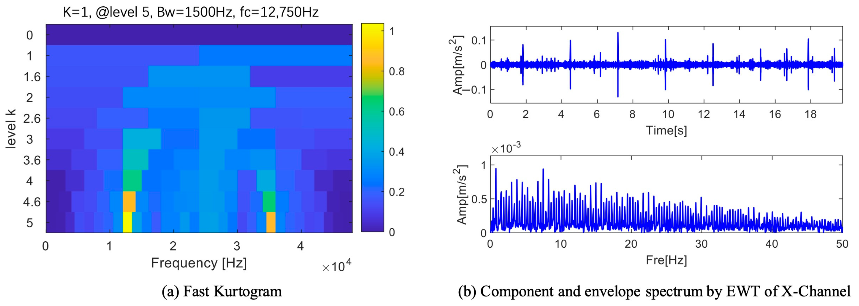
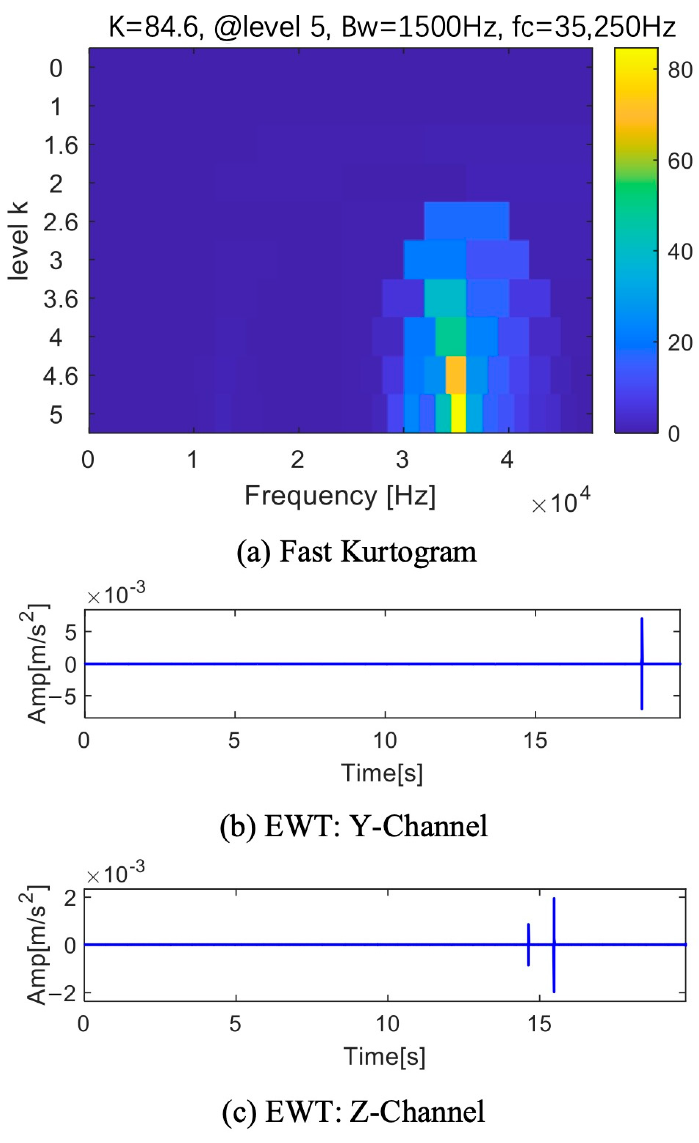
| Number | EWT X-Channel | EWT Y-Channel | EWT Z-Channel | FK Lv4 | MFAMD |
|---|---|---|---|---|---|
| Total Boundaries | 6 | 5 | 2 | 3 | 2 |
| Effective impact | 1 | 1 | 1 | 0 | 6 |
| Channel | Important Frequencies (Hz) | ||
|---|---|---|---|
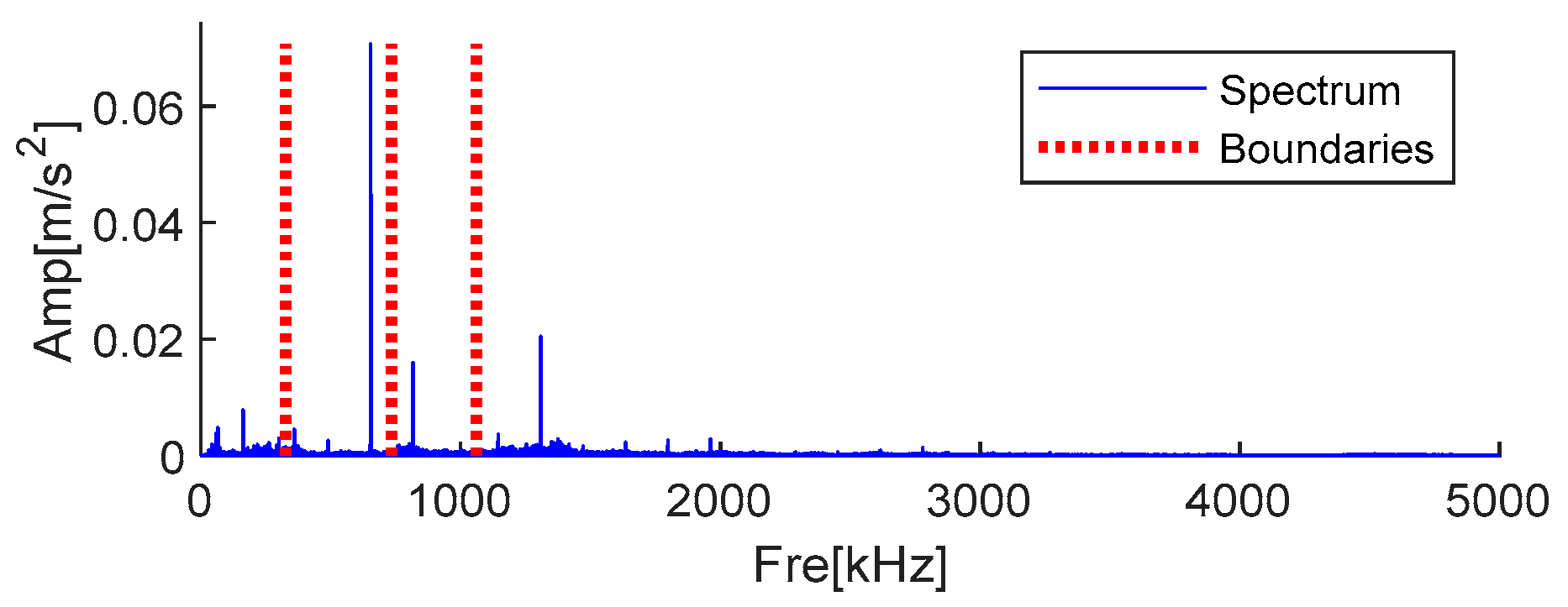
| X | 653.912 | 817.415 | 1307.870 |
| Y | 653.760 | 817.112 | 1307.520 |
| Z | 653.608 | 816.960 | 1307.170 |
Disclaimer/Publisher’s Note: The statements, opinions and data contained in all publications are solely those of the individual author(s) and contributor(s) and not of MDPI and/or the editor(s). MDPI and/or the editor(s) disclaim responsibility for any injury to people or property resulting from any ideas, methods, instructions or products referred to in the content. |
© 2025 by the authors. Licensee MDPI, Basel, Switzerland. This article is an open access article distributed under the terms and conditions of the Creative Commons Attribution (CC BY) license (https://creativecommons.org/licenses/by/4.0/).
Share and Cite
Liu, Y.; Zhang, K.; Yang, M.; Zhang, X.; Xu, Y. Identification of Defects in Low-Speed and Heavy-Load Mechanical Systems Using Multi-Fusion Analytic Mode Decomposition Method. Sensors 2025, 25, 1848. https://doi.org/10.3390/s25061848
Liu Y, Zhang K, Yang M, Zhang X, Xu Y. Identification of Defects in Low-Speed and Heavy-Load Mechanical Systems Using Multi-Fusion Analytic Mode Decomposition Method. Sensors. 2025; 25(6):1848. https://doi.org/10.3390/s25061848
Chicago/Turabian StyleLiu, Yanlei, Kun Zhang, Miaorui Yang, Xu Zhang, and Yonggang Xu. 2025. "Identification of Defects in Low-Speed and Heavy-Load Mechanical Systems Using Multi-Fusion Analytic Mode Decomposition Method" Sensors 25, no. 6: 1848. https://doi.org/10.3390/s25061848
APA StyleLiu, Y., Zhang, K., Yang, M., Zhang, X., & Xu, Y. (2025). Identification of Defects in Low-Speed and Heavy-Load Mechanical Systems Using Multi-Fusion Analytic Mode Decomposition Method. Sensors, 25(6), 1848. https://doi.org/10.3390/s25061848