Figure 1.
The process of wavelet threshold denoising.
Figure 1.
The process of wavelet threshold denoising.
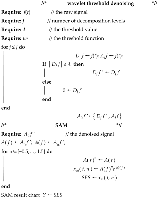
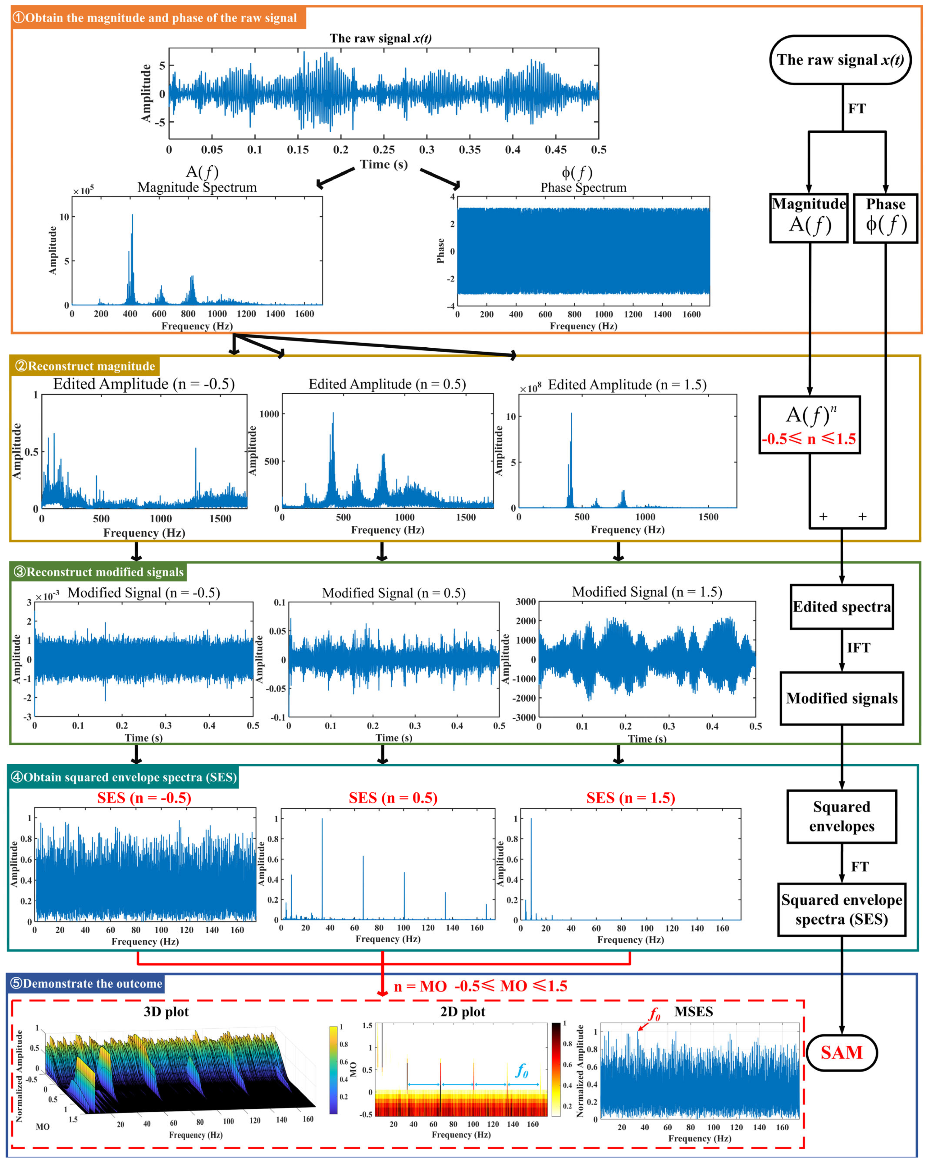
Figure 2.
The diagram of SAM.
Figure 2.
The diagram of SAM.
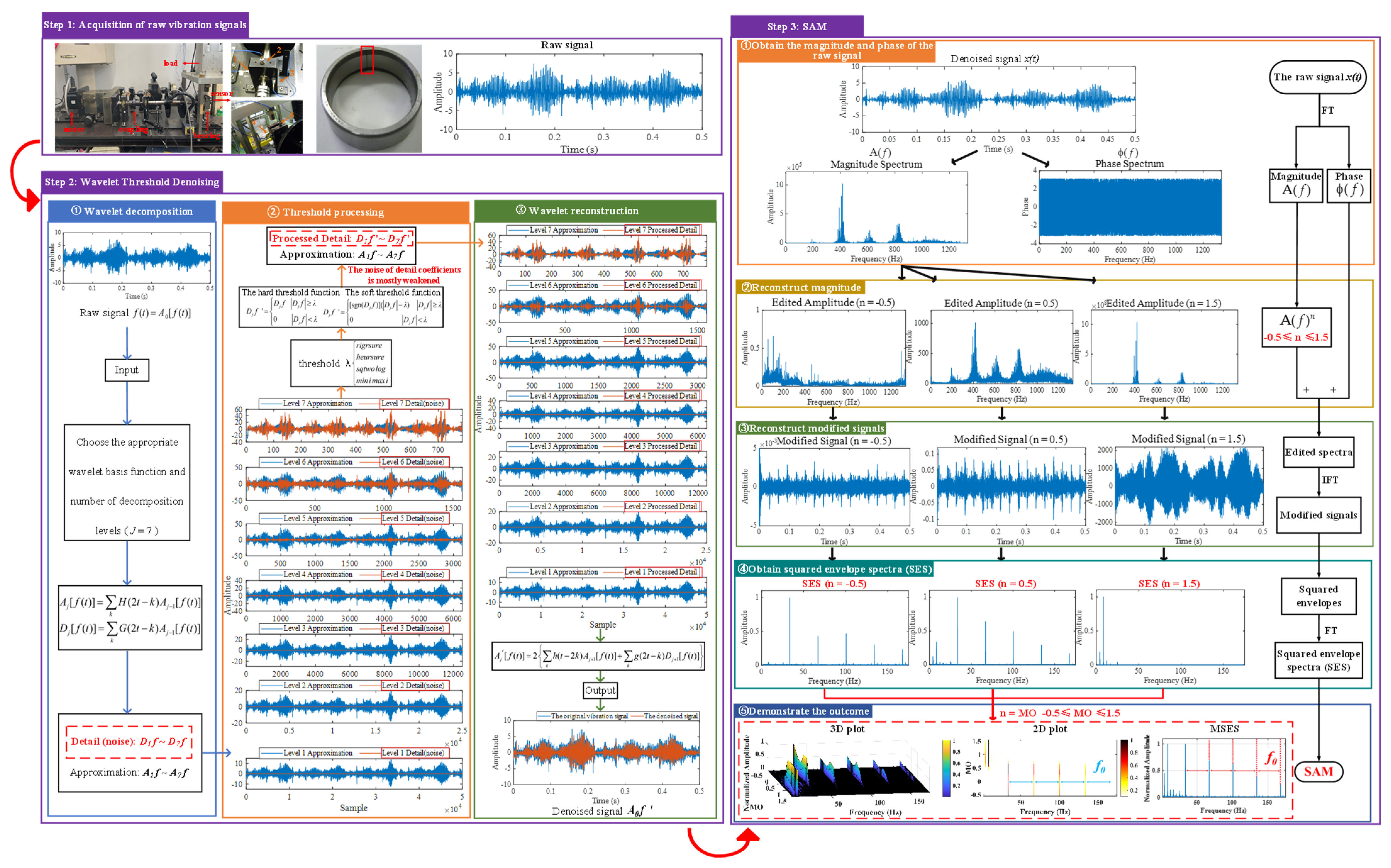
Figure 3.
The process of the proposed method.
Figure 3.
The process of the proposed method.
Figure 4.
Simulated signal. (a) The bearing outer ring fault impulse signal. (b) The harmonic interference signal. (c) The Gaussian white noise. (d) Comparison between the simulated signal and the bearing outer ring fault impulse signal.
Figure 4.
Simulated signal. (a) The bearing outer ring fault impulse signal. (b) The harmonic interference signal. (c) The Gaussian white noise. (d) Comparison between the simulated signal and the bearing outer ring fault impulse signal.
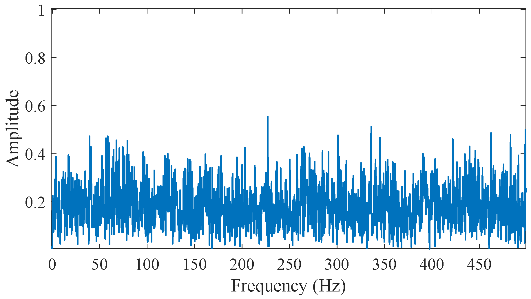
Figure 5.
The envelope spectrum of the raw simulated signal.
Figure 5.
The envelope spectrum of the raw simulated signal.
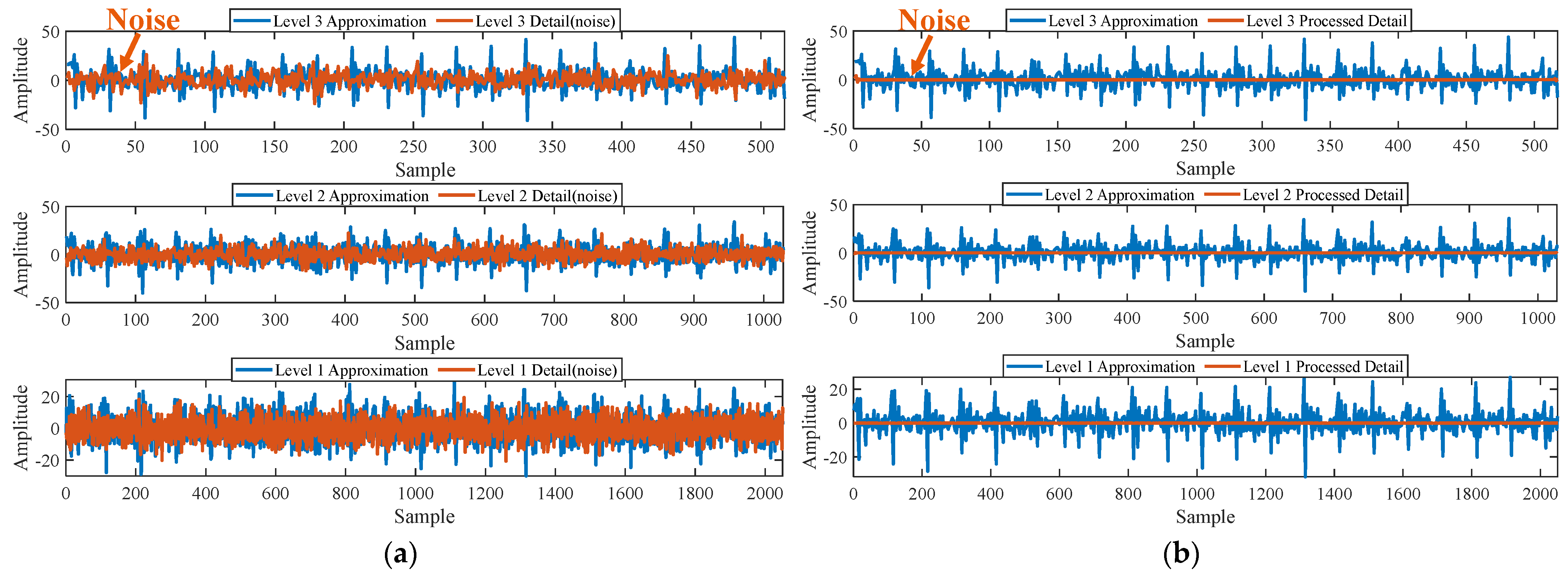
Figure 6.
(a) The approximate part and the detailed part of the wavelet coefficients at levels 1 to 3. (b) The approximate part and the processed detailed part of the wavelet coefficients at levels 1 to 3.
Figure 6.
(a) The approximate part and the detailed part of the wavelet coefficients at levels 1 to 3. (b) The approximate part and the processed detailed part of the wavelet coefficients at levels 1 to 3.
Figure 7.
Comparison between the simulated signal and the denoised signal.
Figure 7.
Comparison between the simulated signal and the denoised signal.
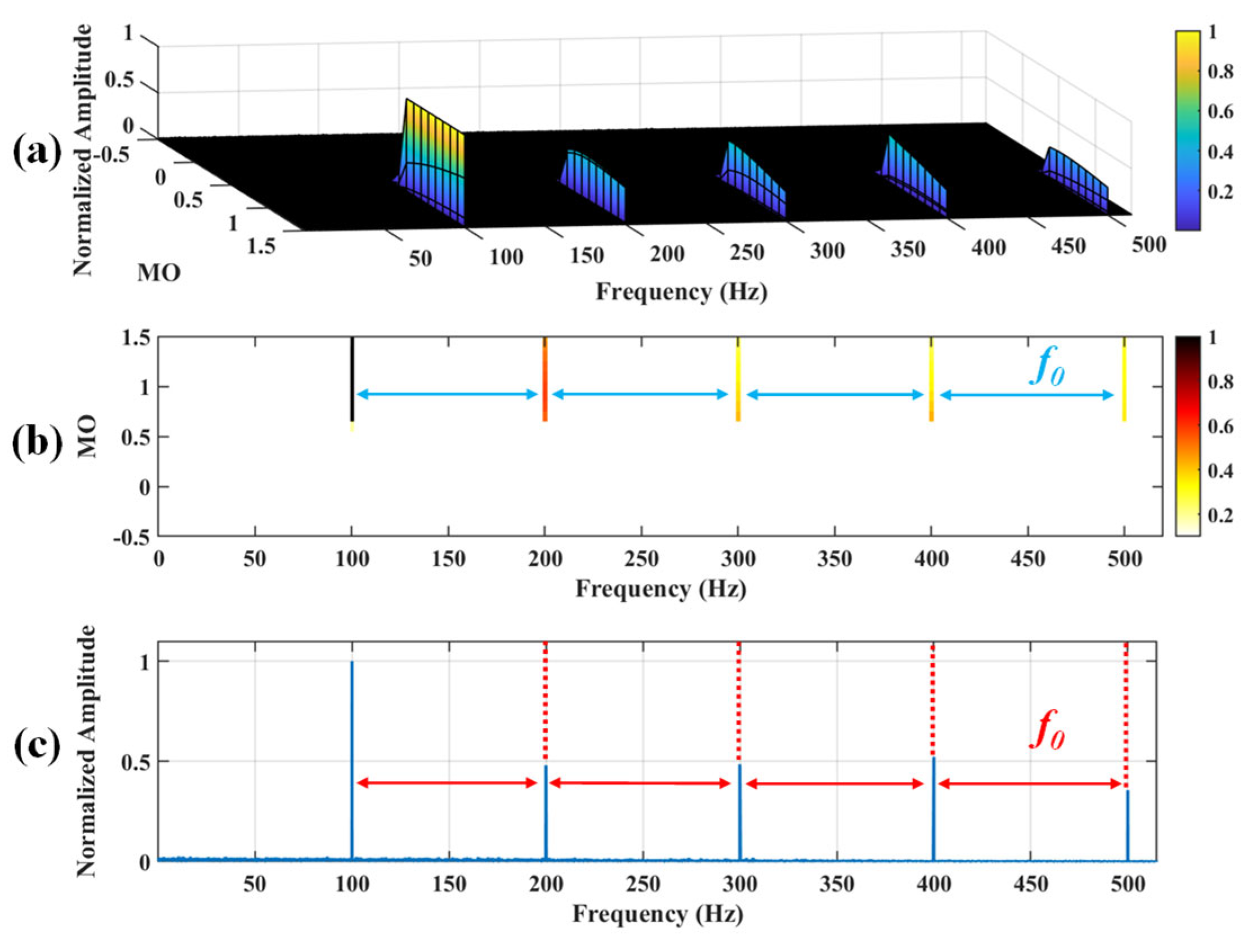
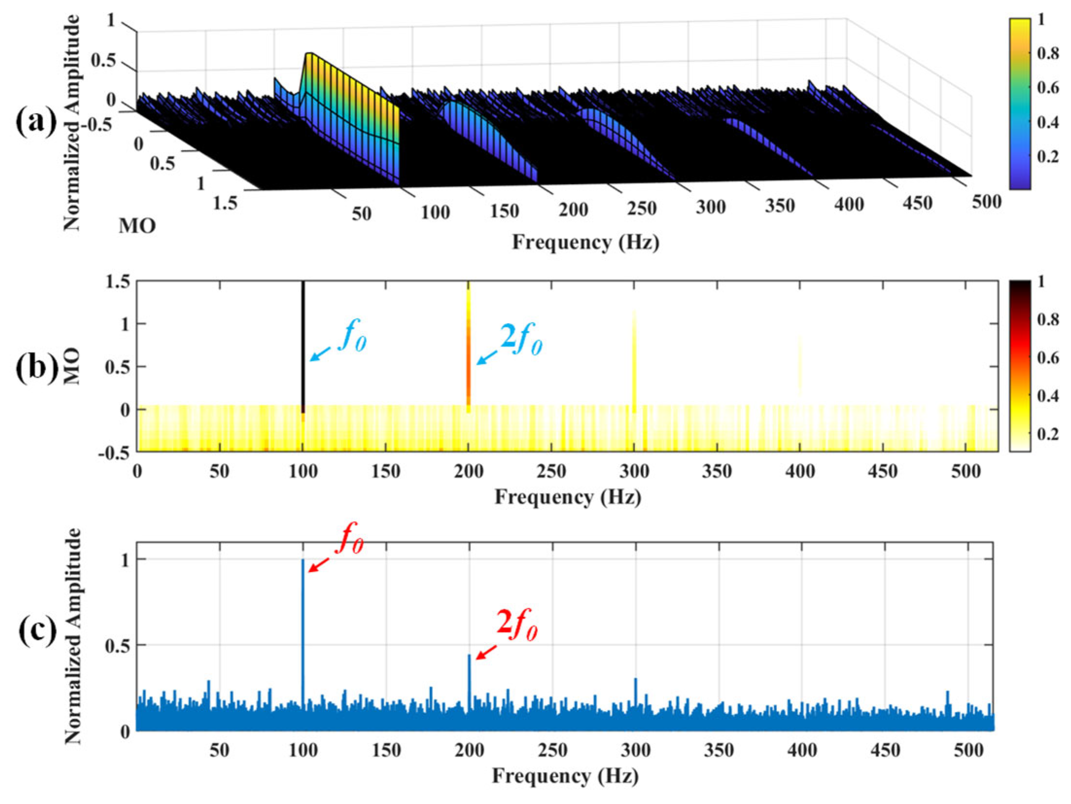
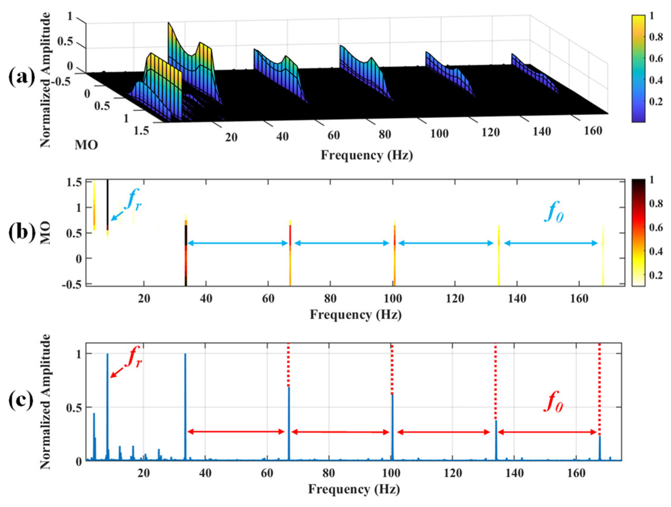
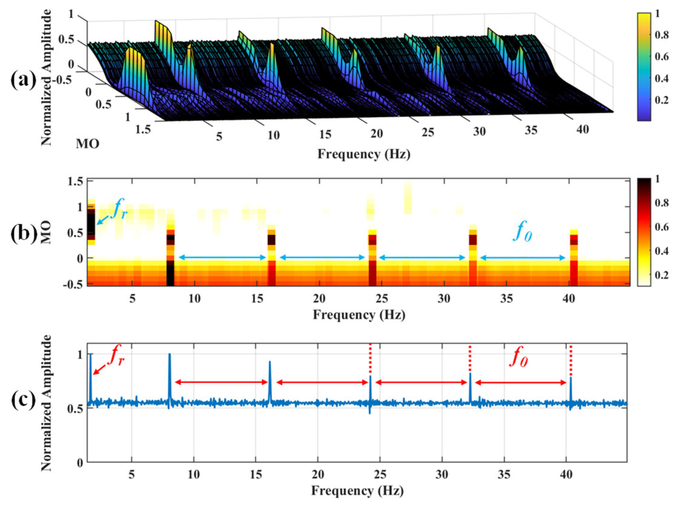
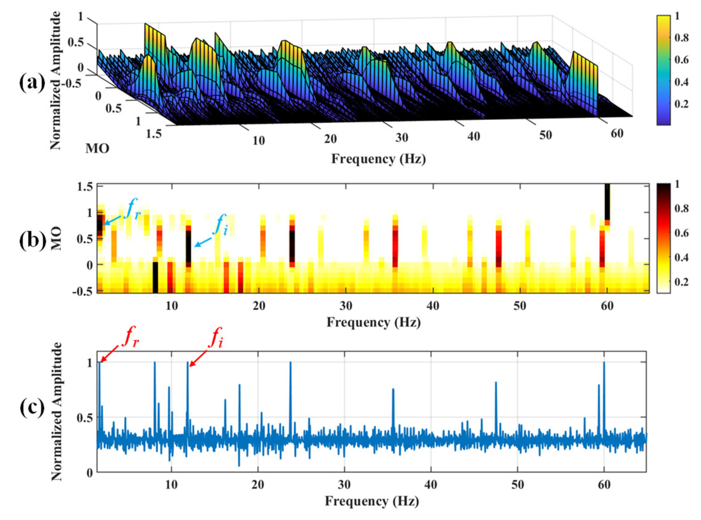
Figure 8.
The demonstration of WTD-SAM. (a) The 3D plot. (b) The 2D plot. (c) The MSES.
Figure 8.
The demonstration of WTD-SAM. (a) The 3D plot. (b) The 2D plot. (c) The MSES.
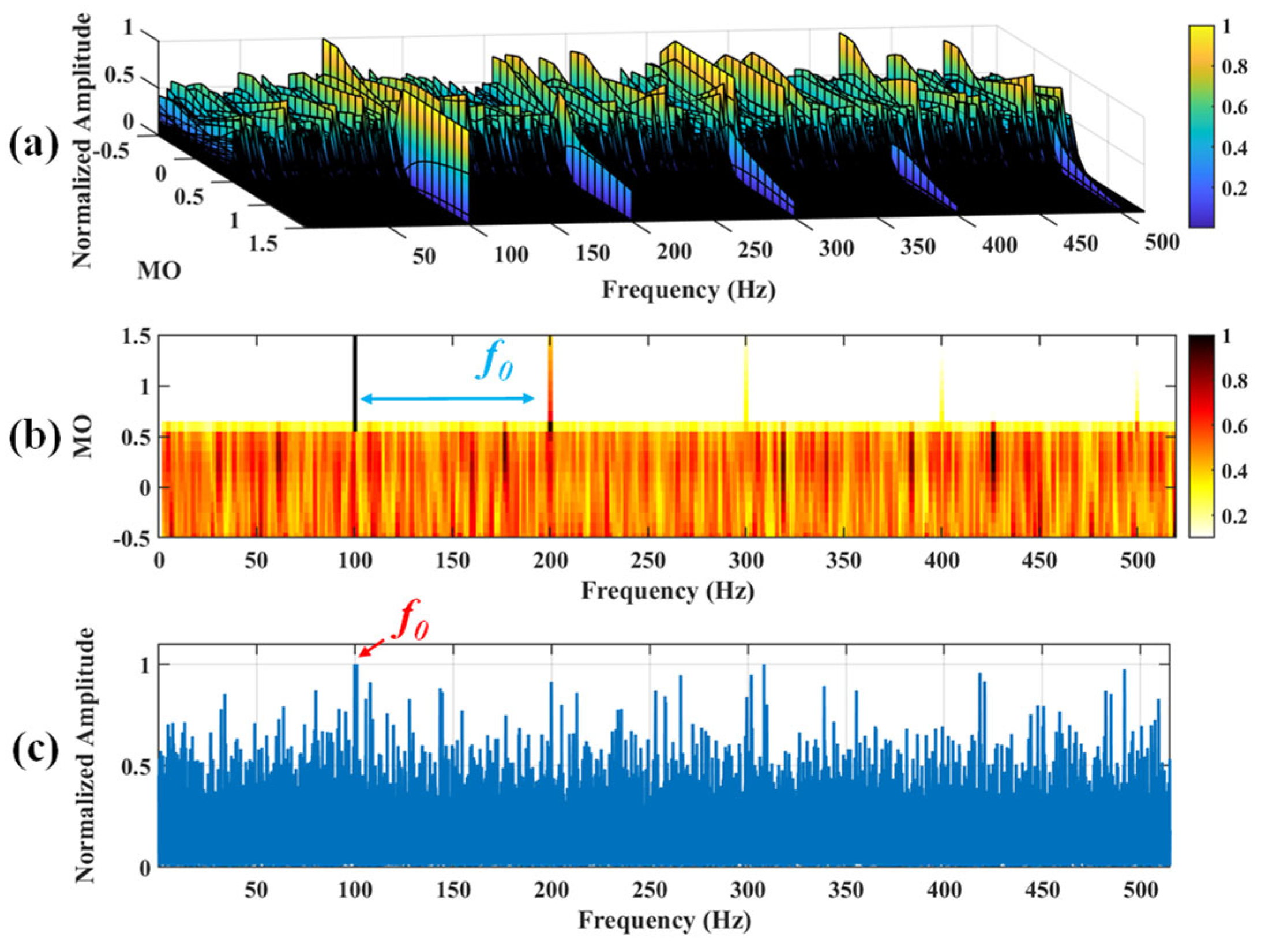
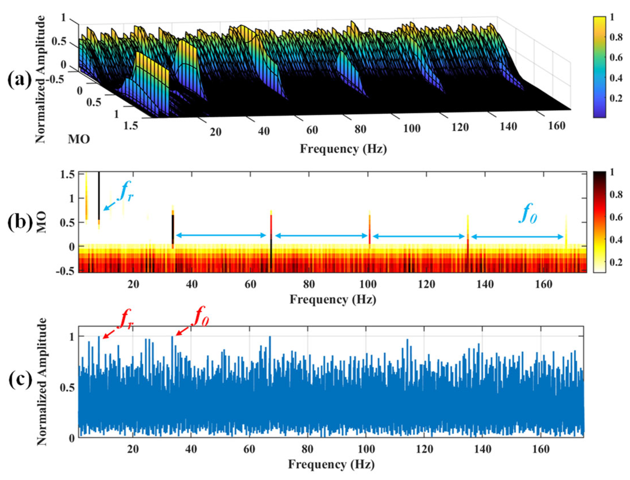
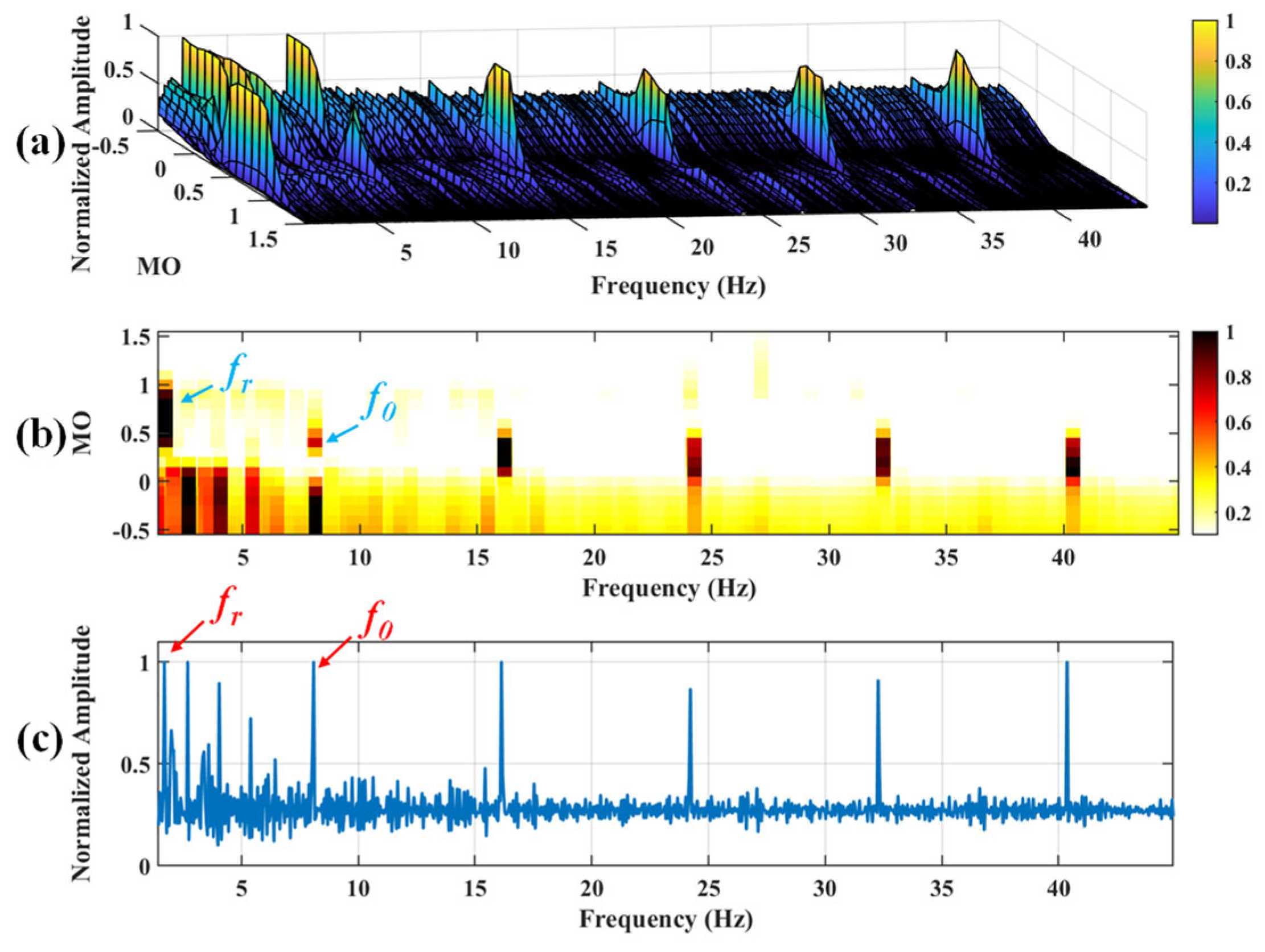
Figure 9.
The demonstration of SAM. (a) The 3D plot. (b) The 2D plot. (c) The MSES.
Figure 9.
The demonstration of SAM. (a) The 3D plot. (b) The 2D plot. (c) The MSES.
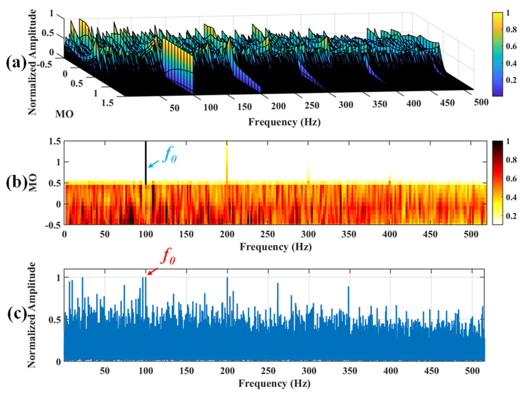
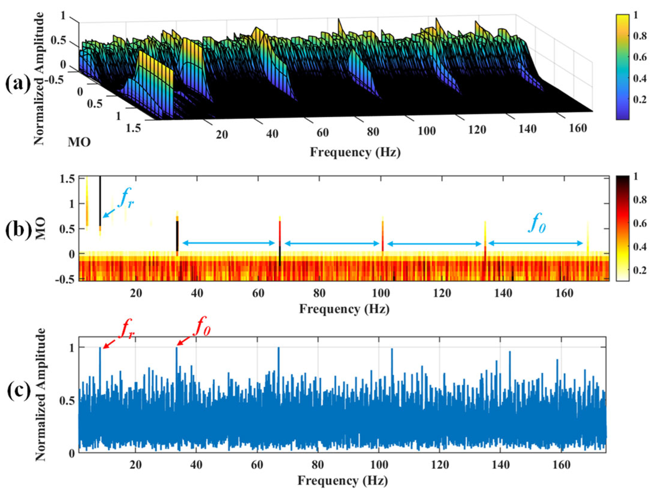
Figure 10.
The demonstration of VMD-SAM. (a) The 3D plot. (b) The 2D plot. (c) The MSES.
Figure 10.
The demonstration of VMD-SAM. (a) The 3D plot. (b) The 2D plot. (c) The MSES.
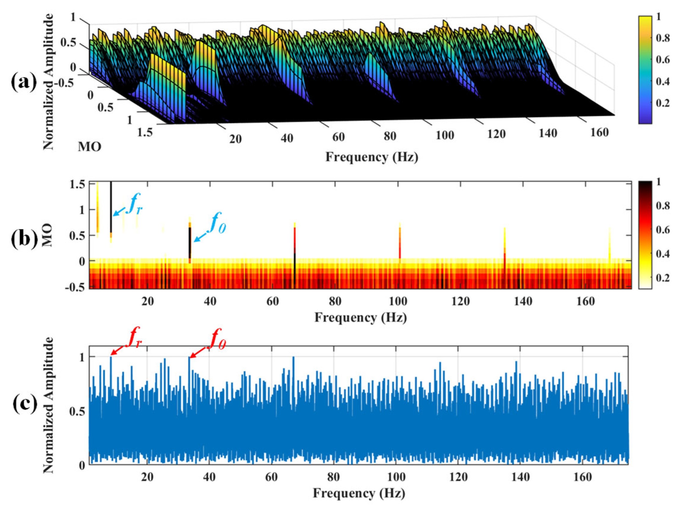
Figure 11.
The demonstration of EMD-SAM. (a) The 3D plot. (b) The 2D plot. (c) The MSES.
Figure 11.
The demonstration of EMD-SAM. (a) The 3D plot. (b) The 2D plot. (c) The MSES.
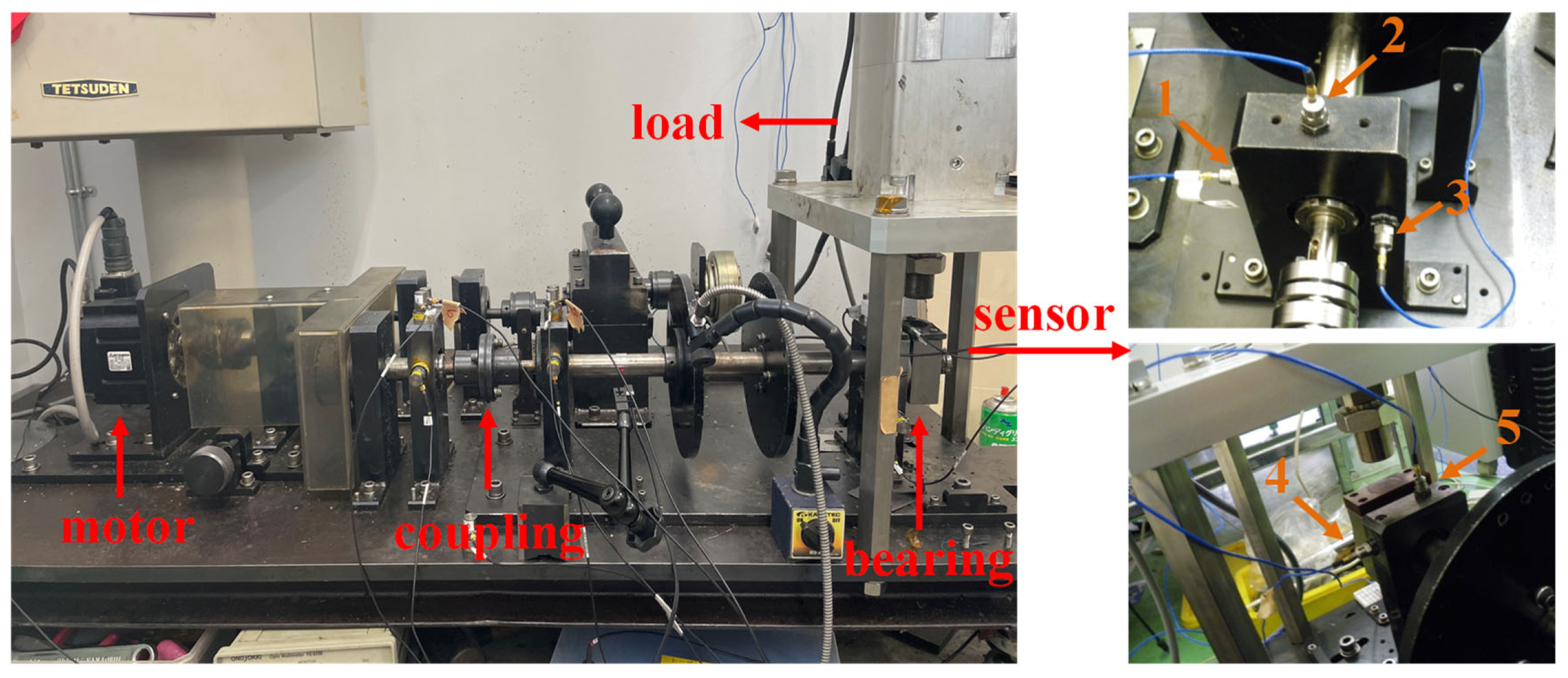
Figure 12.
Experimental platforms.
Figure 12.
Experimental platforms.
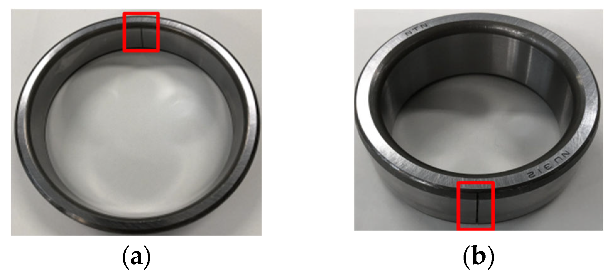
Figure 13.
(a) Bearing outer fault. (b) Bearing inner fault.
Figure 13.
(a) Bearing outer fault. (b) Bearing inner fault.
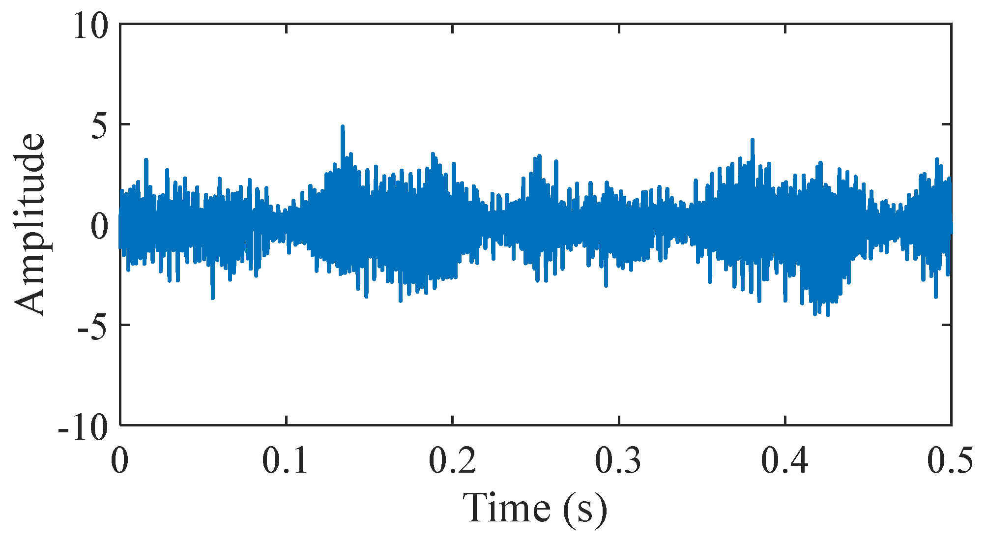
Figure 14.
The bearing signal under normal conditions.
Figure 14.
The bearing signal under normal conditions.
Figure 15.
(a) The approximate part and the detailed part of the wavelet coefficients at levels 1 to 7. (b) The approximate part and the processed detailed part of the wavelet coefficients at levels 1 to 7.
Figure 15.
(a) The approximate part and the detailed part of the wavelet coefficients at levels 1 to 7. (b) The approximate part and the processed detailed part of the wavelet coefficients at levels 1 to 7.
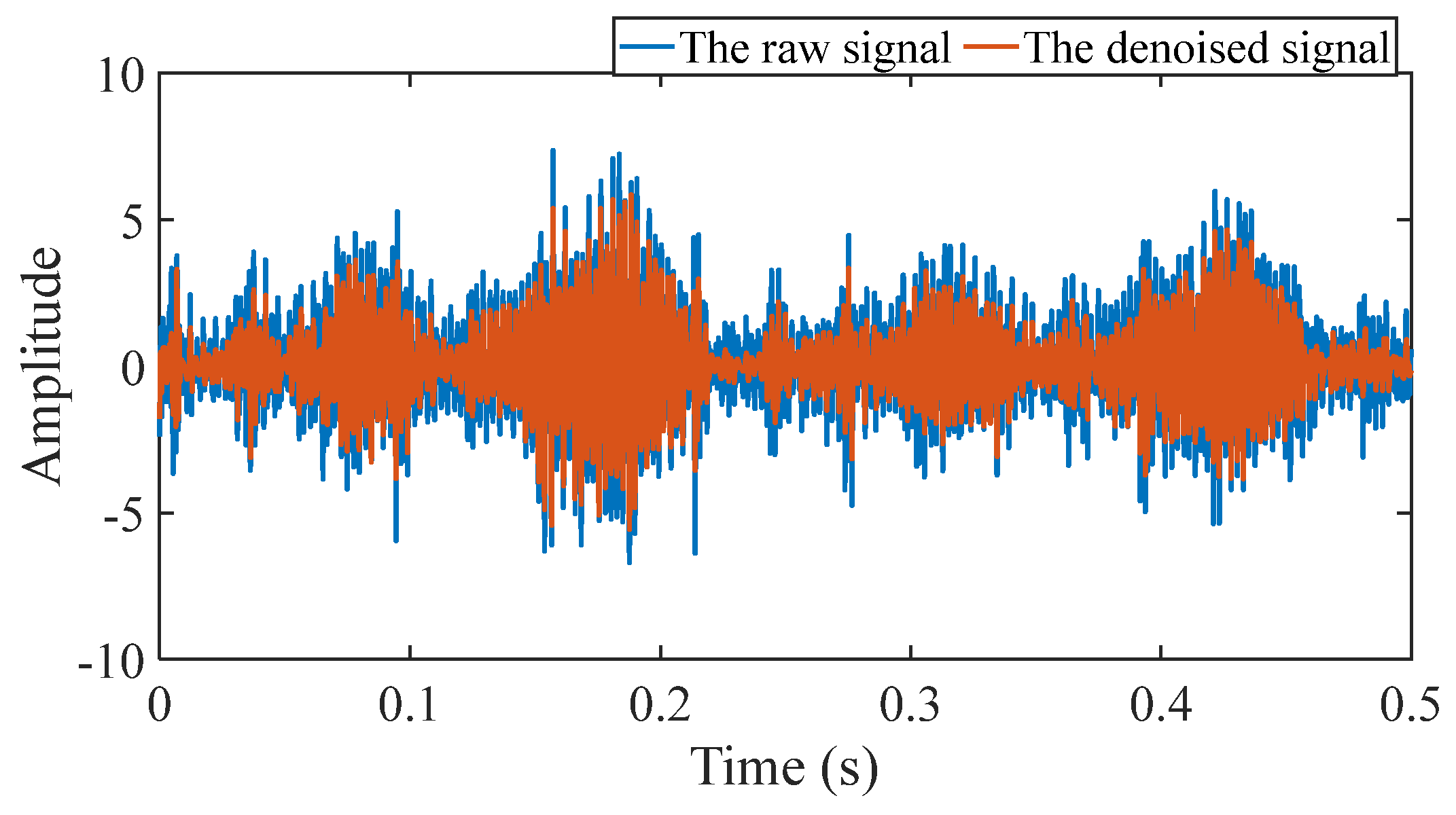
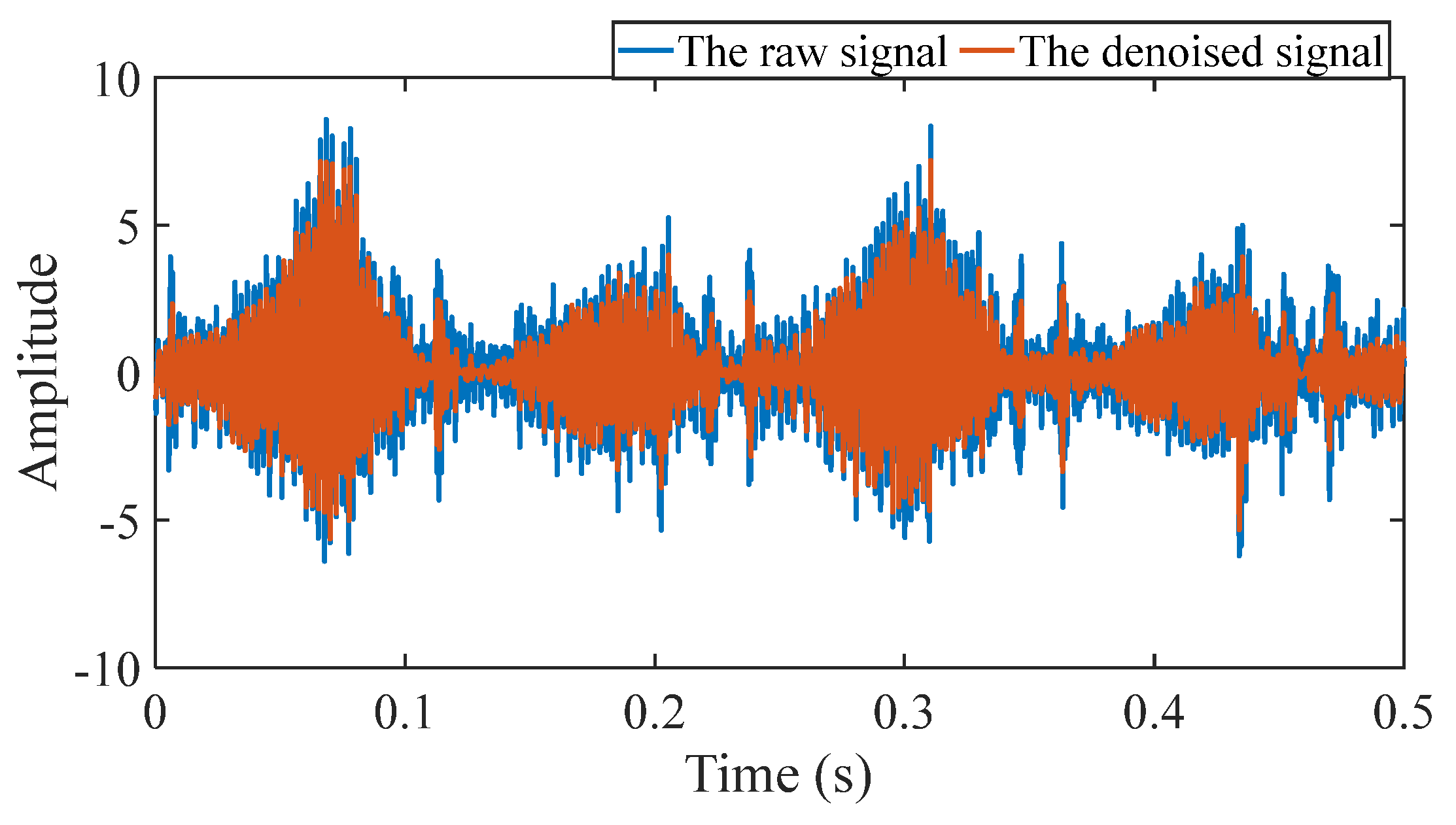
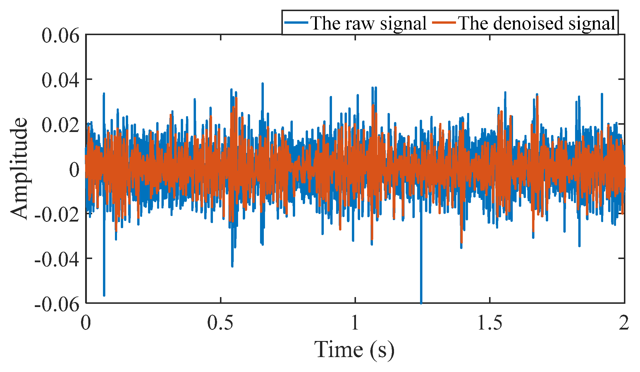
Figure 16.
Comparison between the raw signal and the denoised signal.
Figure 16.
Comparison between the raw signal and the denoised signal.
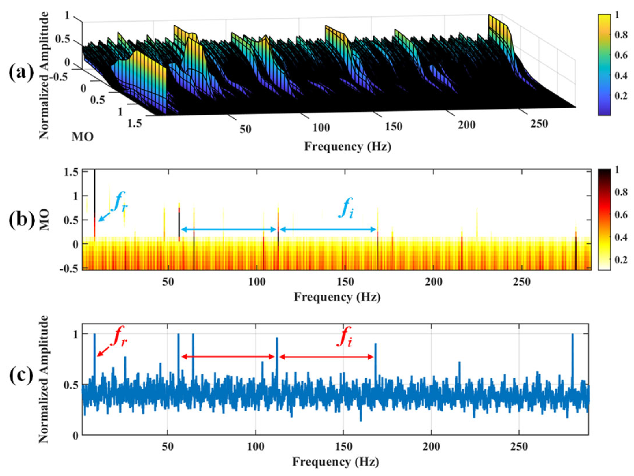
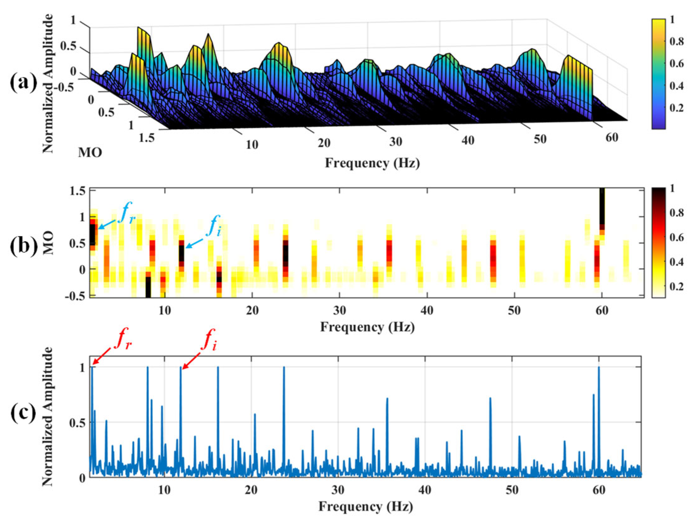
Figure 17.
The demonstration of WTD-SAM. (a) The 3D plot. (b) The 2D plot. (c) The MSES.
Figure 17.
The demonstration of WTD-SAM. (a) The 3D plot. (b) The 2D plot. (c) The MSES.
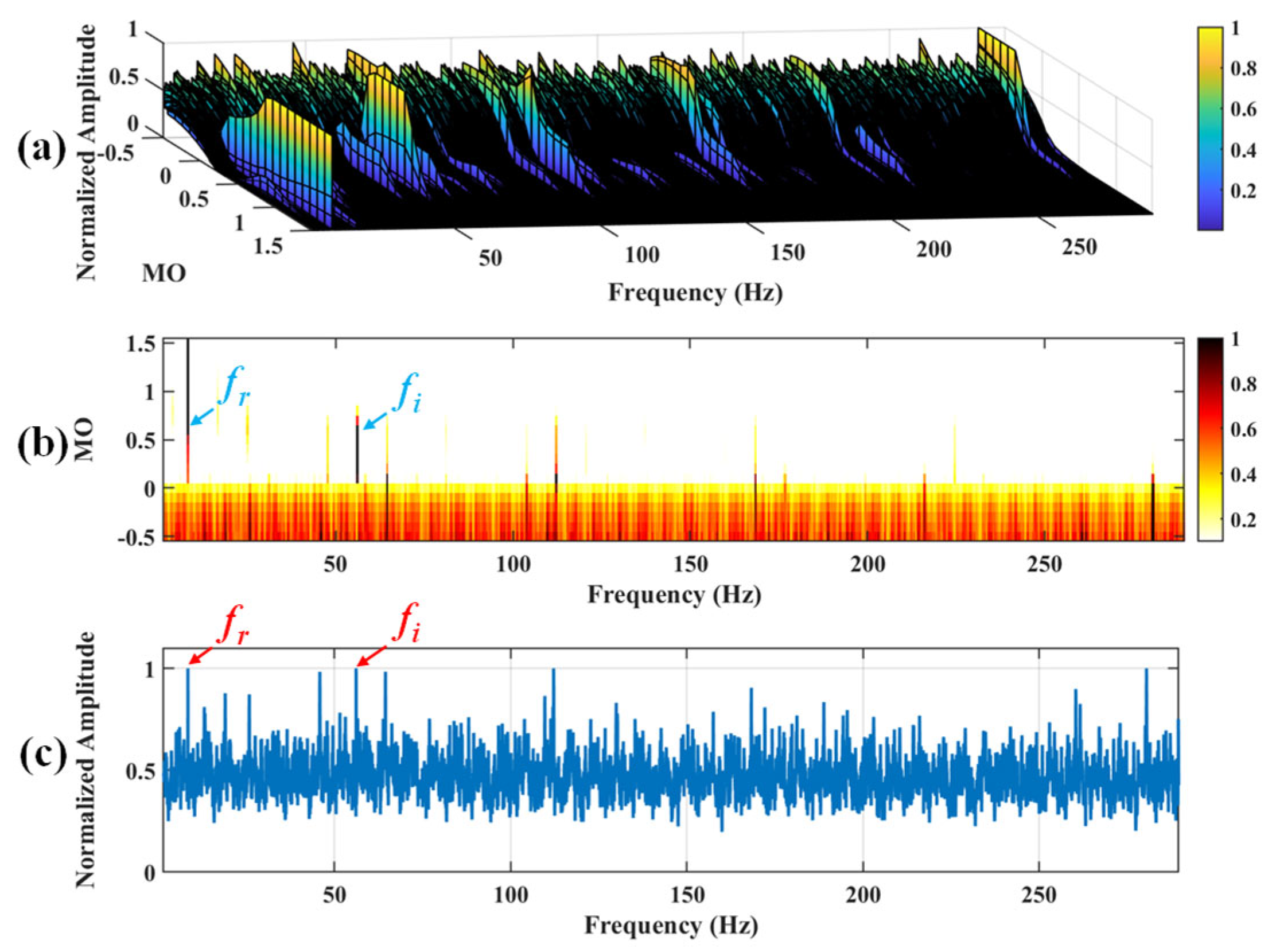
Figure 18.
The demonstration of SAM. (a) The 3D plot. (b) The 2D plot. (c) The MSES.
Figure 18.
The demonstration of SAM. (a) The 3D plot. (b) The 2D plot. (c) The MSES.
Figure 19.
The demonstration of VMD-SAM. (a) The 3D plot. (b) The 2D plot. (c) The MSES.
Figure 19.
The demonstration of VMD-SAM. (a) The 3D plot. (b) The 2D plot. (c) The MSES.
Figure 20.
The demonstration of EMD-SAM. (a) The 3D plot. (b) The 2D plot. (c) The MSES.
Figure 20.
The demonstration of EMD-SAM. (a) The 3D plot. (b) The 2D plot. (c) The MSES.
Figure 21.
(a) The approximate part and the detailed part of the wavelet coefficients at levels 1 to 7. (b) The approximate part and the processed detailed part of the wavelet coefficients at levels 1 to 7.
Figure 21.
(a) The approximate part and the detailed part of the wavelet coefficients at levels 1 to 7. (b) The approximate part and the processed detailed part of the wavelet coefficients at levels 1 to 7.
Figure 22.
Comparison between the raw signal and the denoised signal.
Figure 22.
Comparison between the raw signal and the denoised signal.
Figure 23.
The demonstration of WTD-SAM. (a) The 3D plot. (b) The 2D plot. (c) The MSES.
Figure 23.
The demonstration of WTD-SAM. (a) The 3D plot. (b) The 2D plot. (c) The MSES.
Figure 24.
The demonstration of SAM. (a) The 3D plot. (b) The 2D plot. (c) The MSES.
Figure 24.
The demonstration of SAM. (a) The 3D plot. (b) The 2D plot. (c) The MSES.
Figure 25.
The demonstration of VMD-SAM. (a) The 3D plot. (b) The 2D plot. (c) The MSES.
Figure 25.
The demonstration of VMD-SAM. (a) The 3D plot. (b) The 2D plot. (c) The MSES.
Figure 26.
The demonstration of EMD-SAM. (a) The 3D plot. (b) The 2D plot. (c) The MSES.
Figure 26.
The demonstration of EMD-SAM. (a) The 3D plot. (b) The 2D plot. (c) The MSES.
Figure 27.
Experimental platforms.
Figure 27.
Experimental platforms.
Figure 28.
(a) Bearing outer fault. (b) Bearing inner fault.
Figure 28.
(a) Bearing outer fault. (b) Bearing inner fault.
Figure 29.
The bearing signal under normal conditions.
Figure 29.
The bearing signal under normal conditions.
Figure 30.
(a) The approximate part and the detailed part of the wavelet coefficients at levels 1 to 8. (b) The approximate part and the processed detailed part of the wavelet coefficients at levels 1 to 8.
Figure 30.
(a) The approximate part and the detailed part of the wavelet coefficients at levels 1 to 8. (b) The approximate part and the processed detailed part of the wavelet coefficients at levels 1 to 8.
Figure 31.
Comparison between the raw signal and the denoised signal.
Figure 31.
Comparison between the raw signal and the denoised signal.
Figure 32.
The demonstration of WTD-SAM. (a) The 3D plot. (b) The 2D plot. (c) The MSES.
Figure 32.
The demonstration of WTD-SAM. (a) The 3D plot. (b) The 2D plot. (c) The MSES.
Figure 33.
The demonstration of SAM. (a) The 3D plot. (b) The 2D plot. (c) The MSES.
Figure 33.
The demonstration of SAM. (a) The 3D plot. (b) The 2D plot. (c) The MSES.
Figure 34.
The demonstration of VMD-SAM. (a) The 3D plot. (b) The 2D plot. (c) The MSES.
Figure 34.
The demonstration of VMD-SAM. (a) The 3D plot. (b) The 2D plot. (c) The MSES.
Figure 35.
The demonstration of EMD-SAM. (a) The 3D plot. (b) The 2D plot. (c) The MSES.
Figure 35.
The demonstration of EMD-SAM. (a) The 3D plot. (b) The 2D plot. (c) The MSES.
Figure 36.
(a) The approximate part and the detailed part of the wavelet coefficients at levels 1 to 8. (b) The approximate part and the processed detailed part of the wavelet coefficients at levels 1 to 8.
Figure 36.
(a) The approximate part and the detailed part of the wavelet coefficients at levels 1 to 8. (b) The approximate part and the processed detailed part of the wavelet coefficients at levels 1 to 8.
Figure 37.
Comparison between the raw signal and the denoised signal.
Figure 37.
Comparison between the raw signal and the denoised signal.
Figure 38.
The demonstration of WTD-SAM. (a) The 3D plot. (b) The 2D plot. (c) The MSES.
Figure 38.
The demonstration of WTD-SAM. (a) The 3D plot. (b) The 2D plot. (c) The MSES.
Figure 39.
The demonstration of SAM. (a) The 3D plot. (b) The 2D plot. (c) The MSES.
Figure 39.
The demonstration of SAM. (a) The 3D plot. (b) The 2D plot. (c) The MSES.
Figure 40.
The demonstration of VMD-SAM. (a) The 3D plot. (b) The 2D plot. (c) The MSES.
Figure 40.
The demonstration of VMD-SAM. (a) The 3D plot. (b) The 2D plot. (c) The MSES.
Figure 41.
The demonstration of EMD-SAM. (a) The 3D plot. (b) The 2D plot. (c) The MSES.
Figure 41.
The demonstration of EMD-SAM. (a) The 3D plot. (b) The 2D plot. (c) The MSES.
Table 1.
Parameters of bearings.
Table 1.
Parameters of bearings.
| Parameter | Value |
|---|
| Defect on outer | 0.3 × 0.05 (width × depth) |
| Defect on inner | 0.3 × 0.05 (width × depth) |
Table 2.
The fault feature frequency of the bearing.
Table 2.
The fault feature frequency of the bearing.
| Speed | f0 | fi |
|---|
| 500 RPM | 36.5956 Hz | 55.0711 Hz |
Table 3.
Parameters of bearings.
Table 3.
Parameters of bearings.
| Parameter | Value |
|---|
| Defect on outer | 0.6 × 0.3 (width × depth) |
| Defect on inner | 0.6 × 0.3 (width × depth) |
Table 4.
The fault feature frequency of the bearing.
Table 4.
The fault feature frequency of the bearing.
| Speed | f0 | fi |
| 100 RPM | 8 Hz | 12 Hz |
Table 5.
The comparison of EFF index.
Table 5.
The comparison of EFF index.
| Speed | Fault Type | WTD-SAM | SAM | VMD-SAM | EMD-SAM |
|---|
| 500 RPM | Outer fault | 62.09 | 6.70 | 7.72 | 6.97 |
| Inner fault | 53.27 | 9.41 | 8.70 | 32.60 |
| 100 RPM | Outer fault | 36.28 | 18.31 | 20.67 | 14.23 |
| Inner fault | 35.73 | 20.23 | 20.29 | 18.06 |
Table 6.
Comparison of time calculation by different methods.
Table 6.
Comparison of time calculation by different methods.
| Speed | Fault Type | WTD-SAM | SAM | VMD-SAM | EMD-SAM |
|---|
| 500 RPM | Outer fault | 3.52 s | 3.02 s | 115.84 s | 4.31 s |
| Inner fault | 3.89 s | 3.16 s | 34.33 s | 4.53 s |
| 100 RPM | Outer fault | 3.94 s | 3.28 s | 49.30 s | 4.89 s |
| Inner fault | 3.51 s | 2.98 s | 47.95 s | 4.33 s |


 ,
, 


