

Evaluation of Long-Term Performance of Six PM2.5 Sensor Types

 ,
, 
Abstract
1. Introduction
2. Materials and Methods
2.1. Study Design Overview
2.2. Sensors Selected
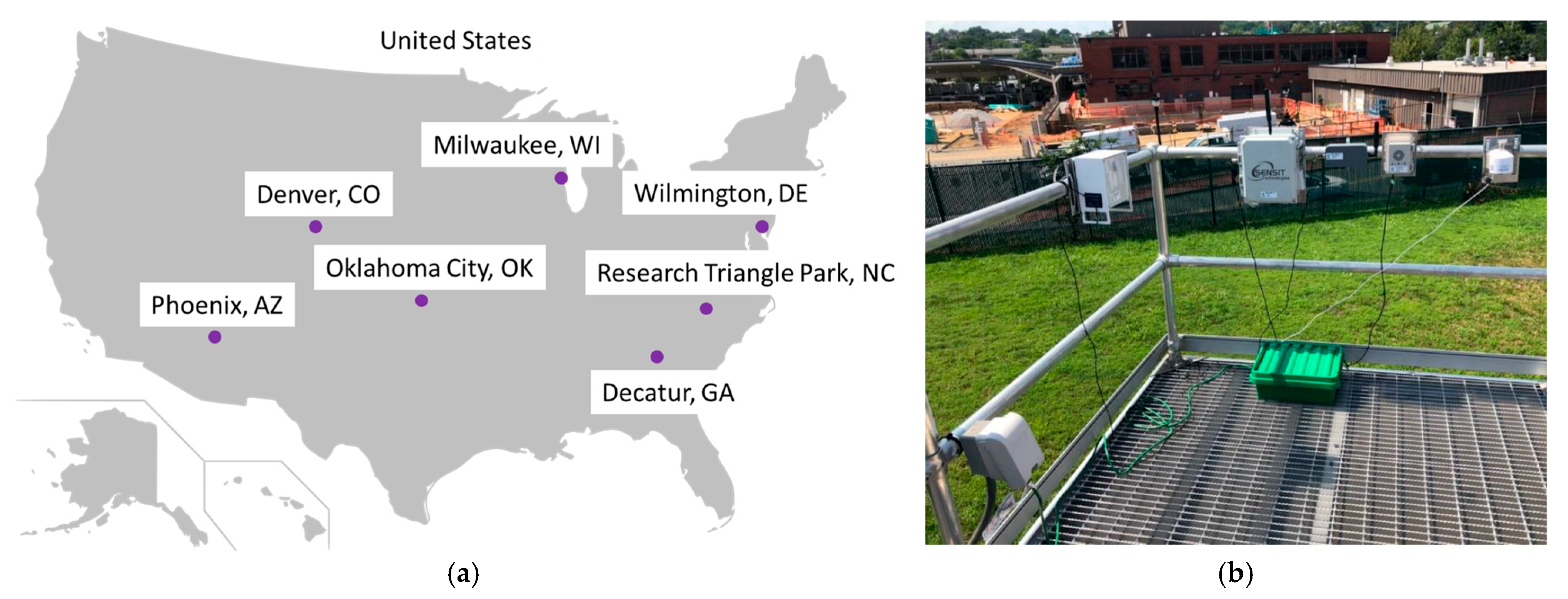
2.3. Long-Term Monitoring Sites Selected
2.4. Data Processing and Analysis
3. Results and Discussion
3.1. Common Failure Points
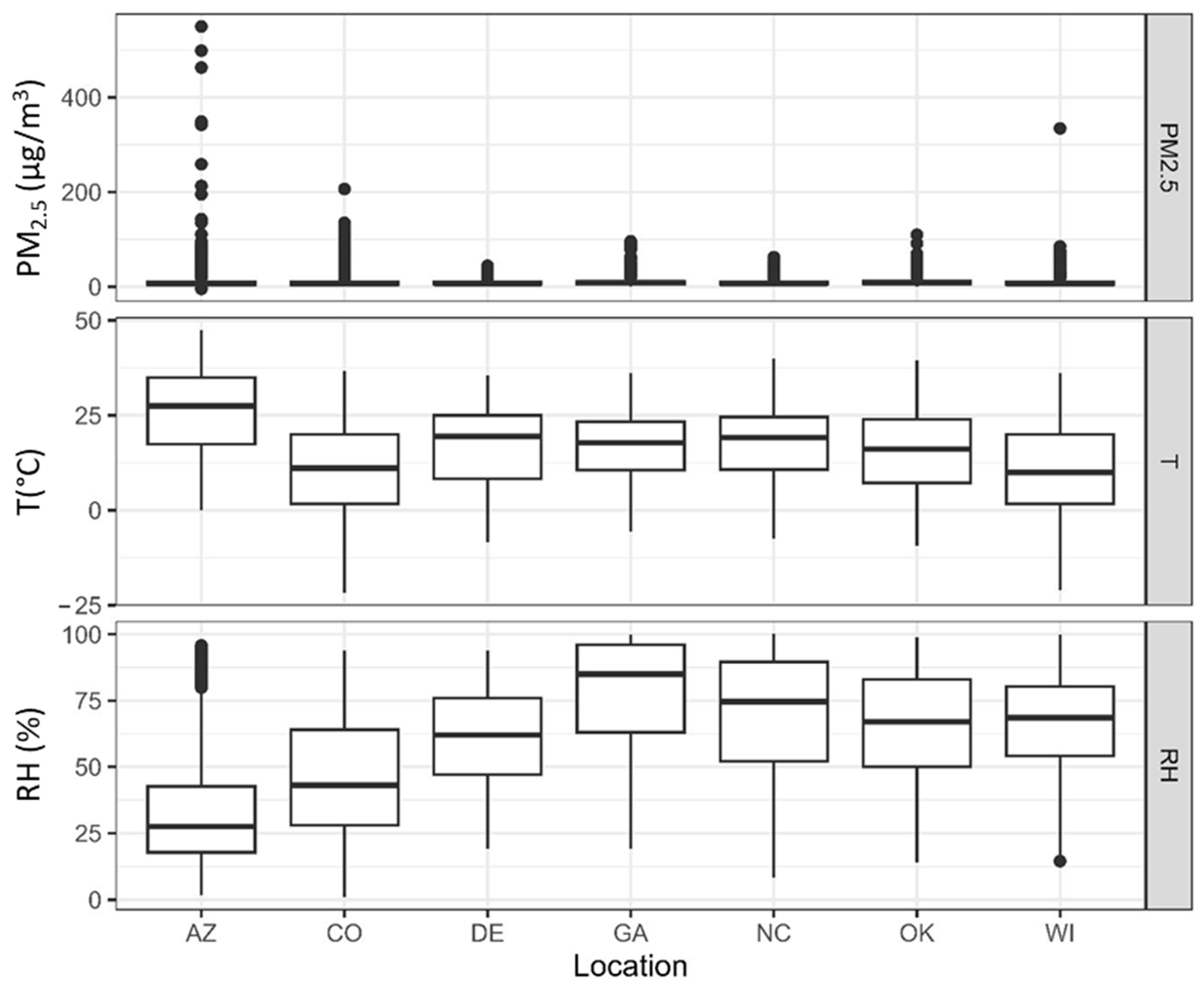
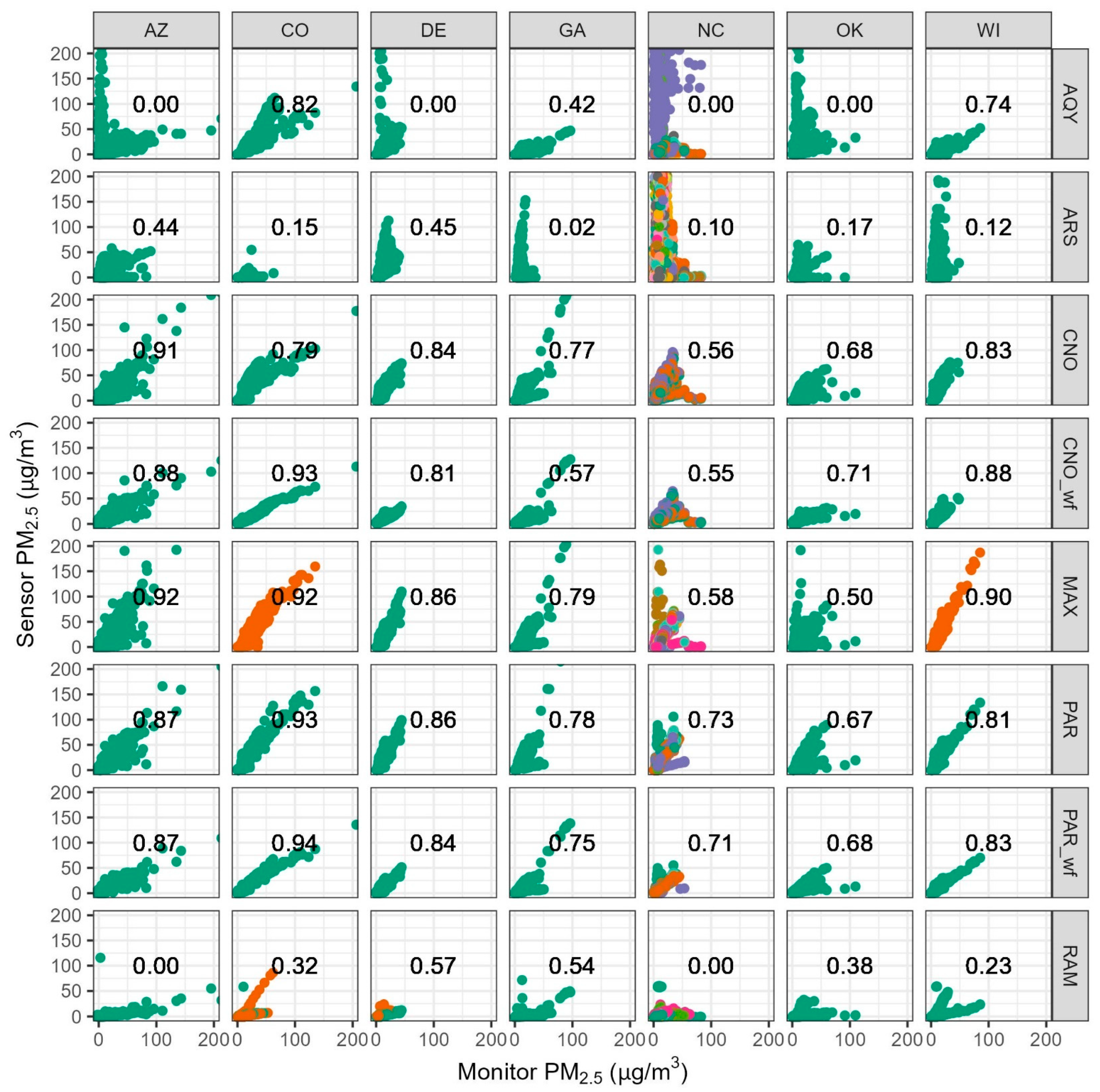
3.2. Overall Performance by Site
3.3. Common Data Issues
3.3.1. Zero
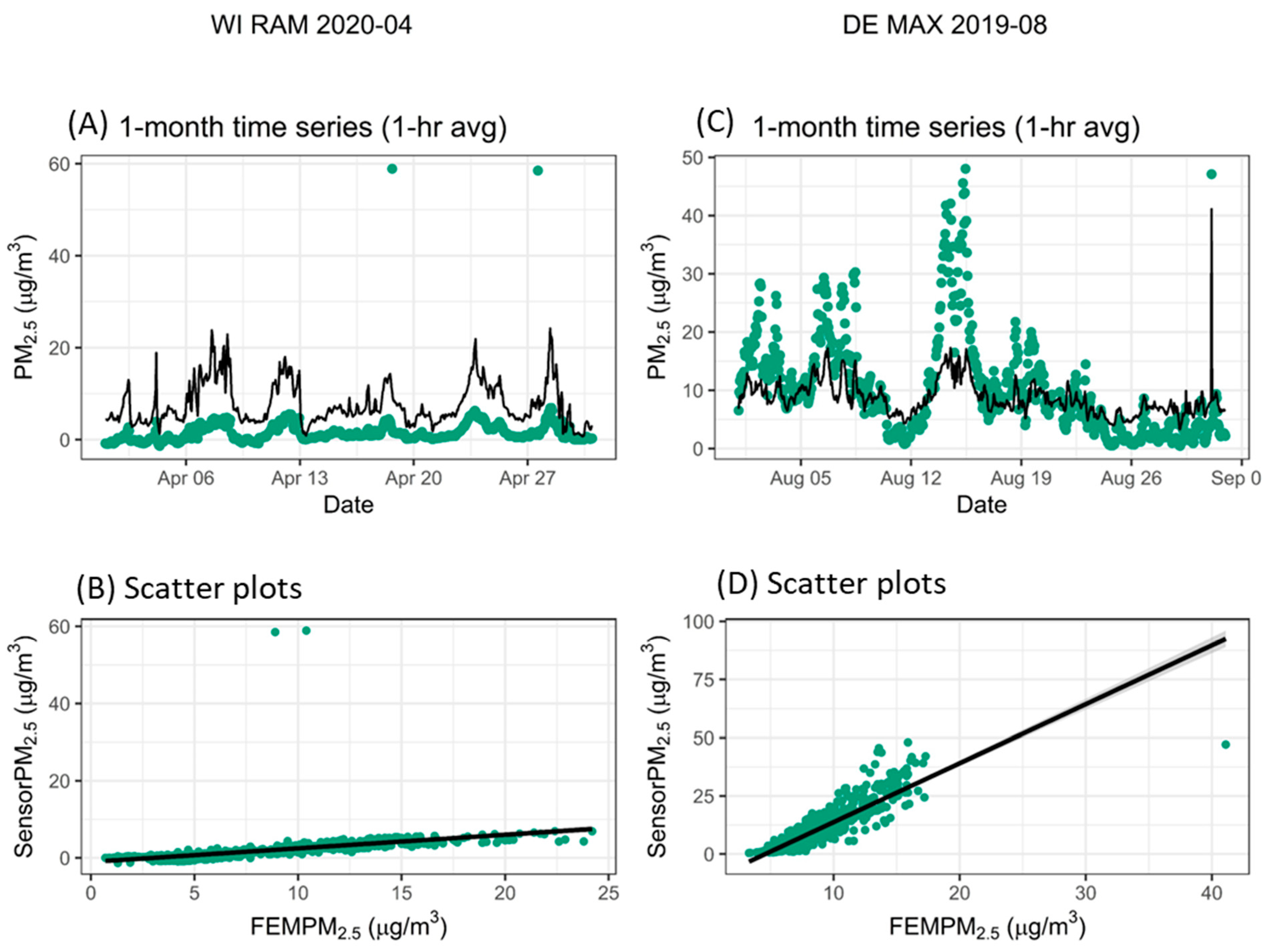
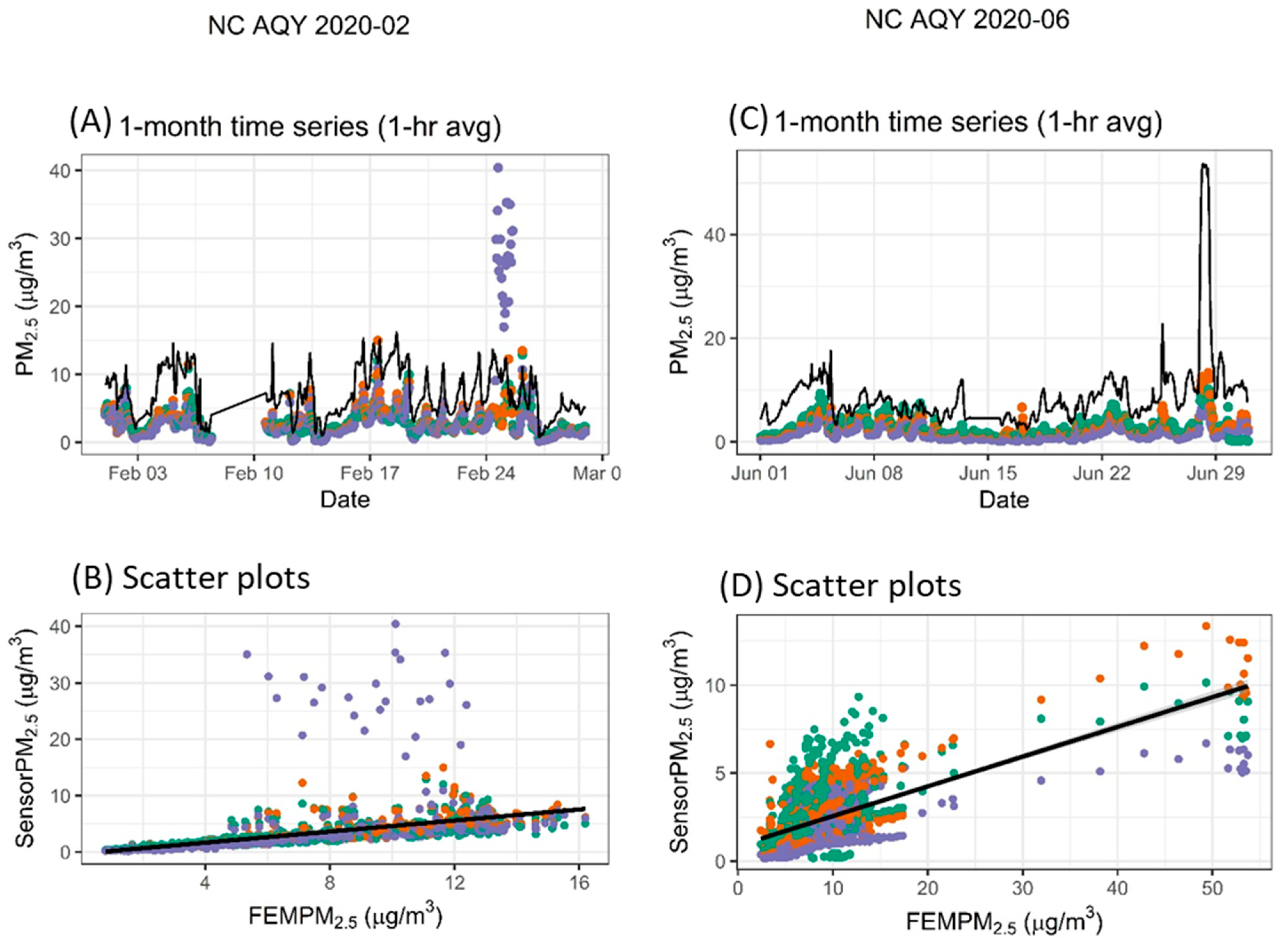
3.3.2. Outlier
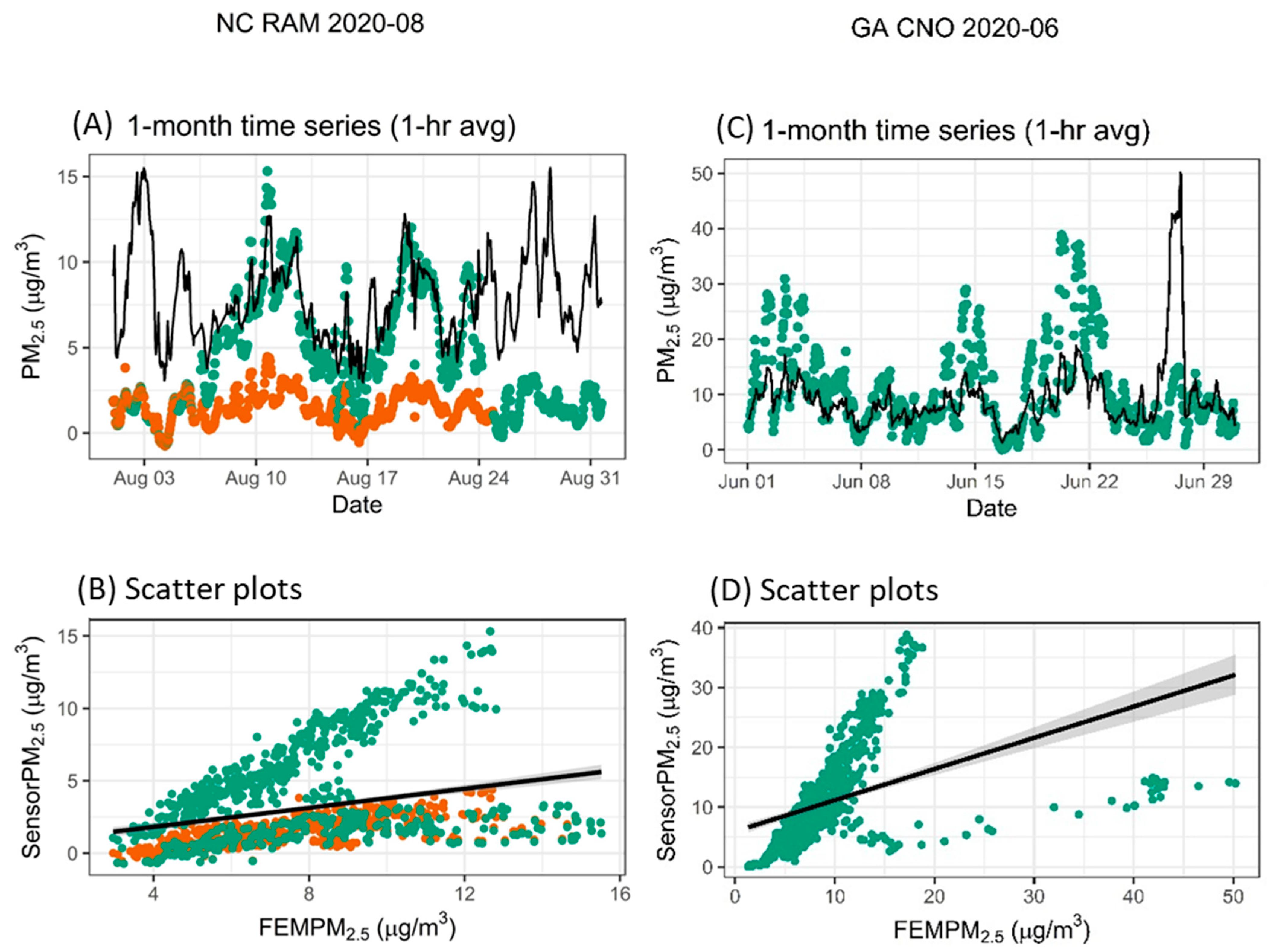
3.3.3. Baseline Shift
3.3.4. Variable Relationship Between Sensor and Monitor
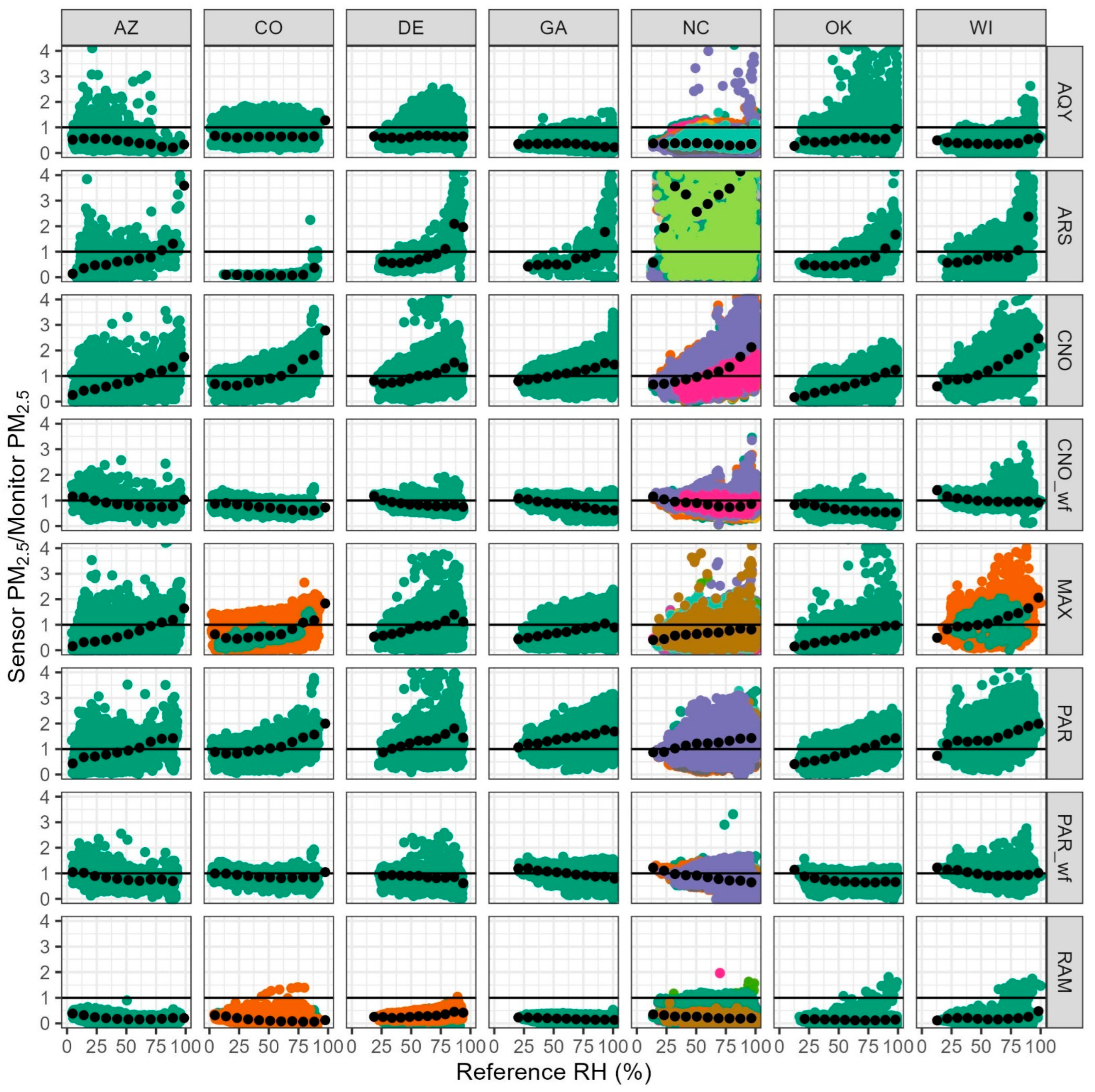
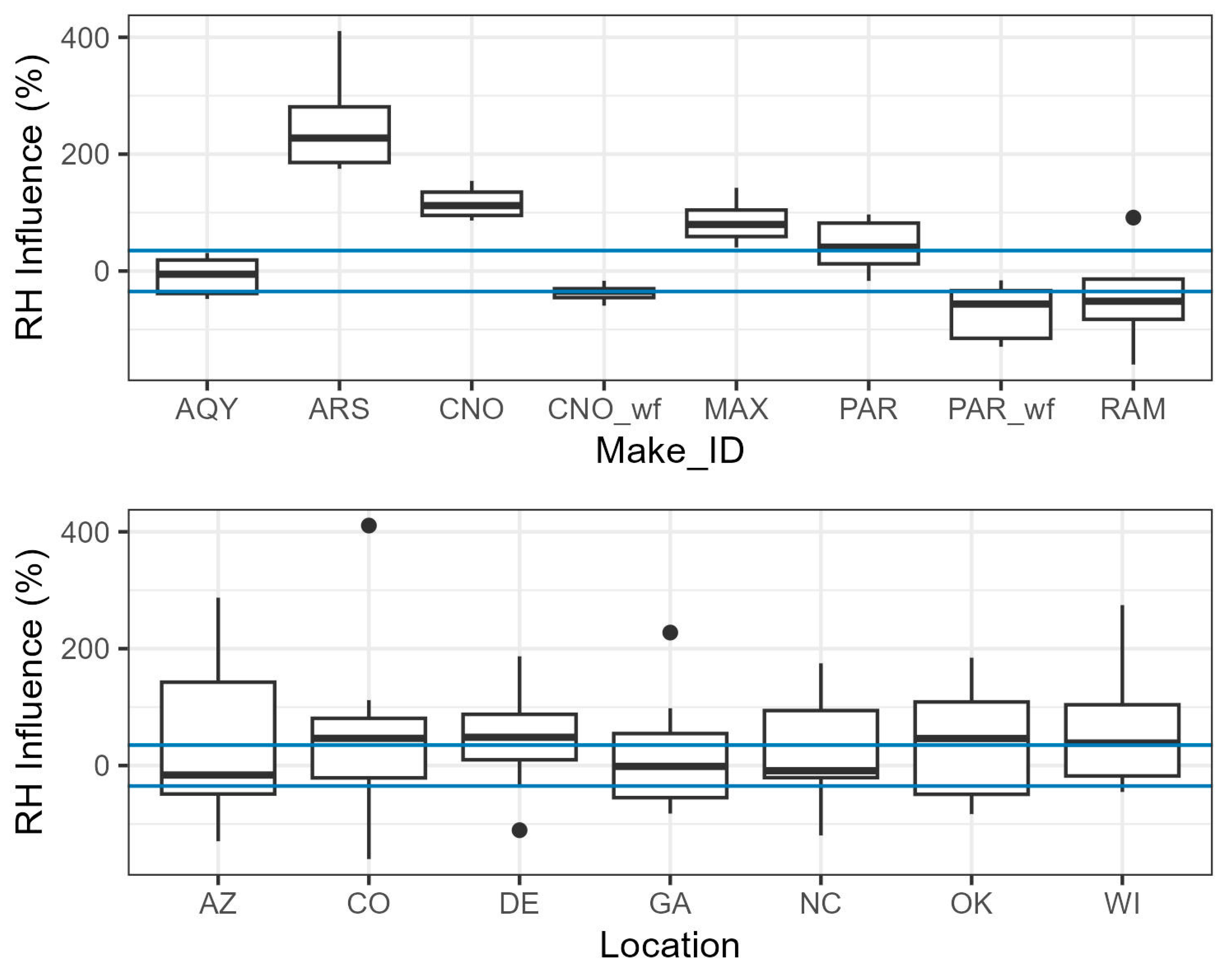
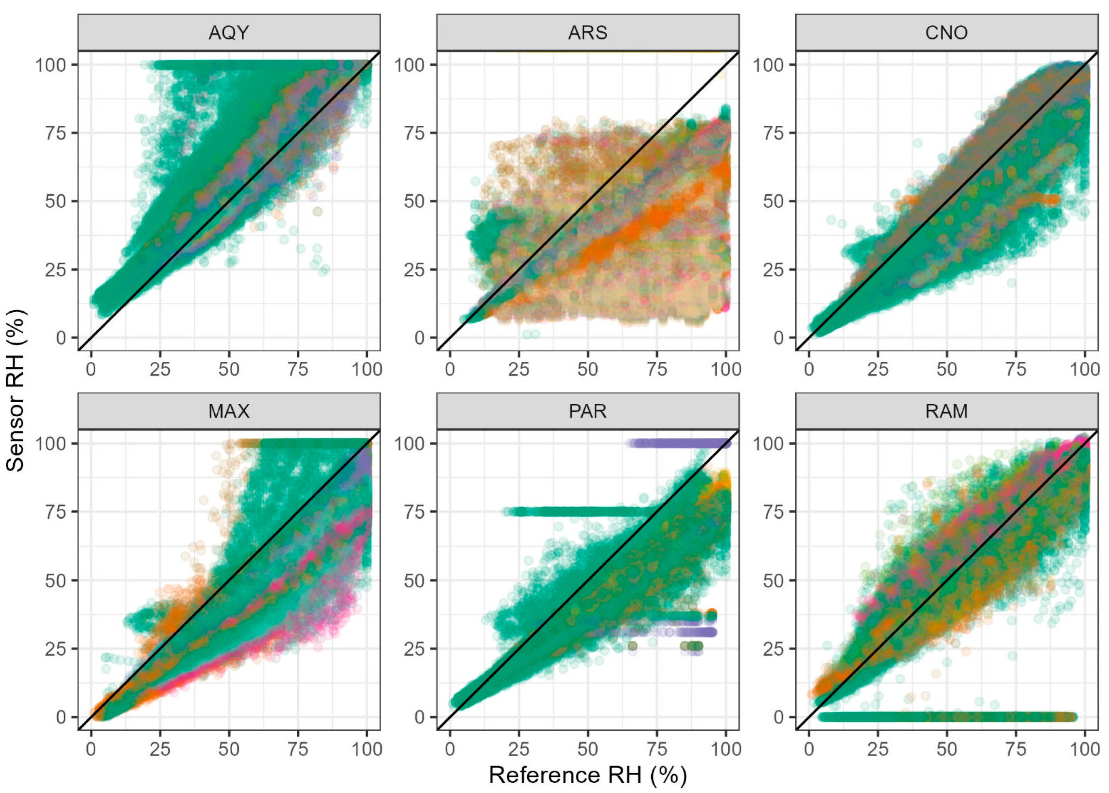
3.4. RH Influence
3.5. Variability in Bias
3.5.1. Bias by Sensor and Location
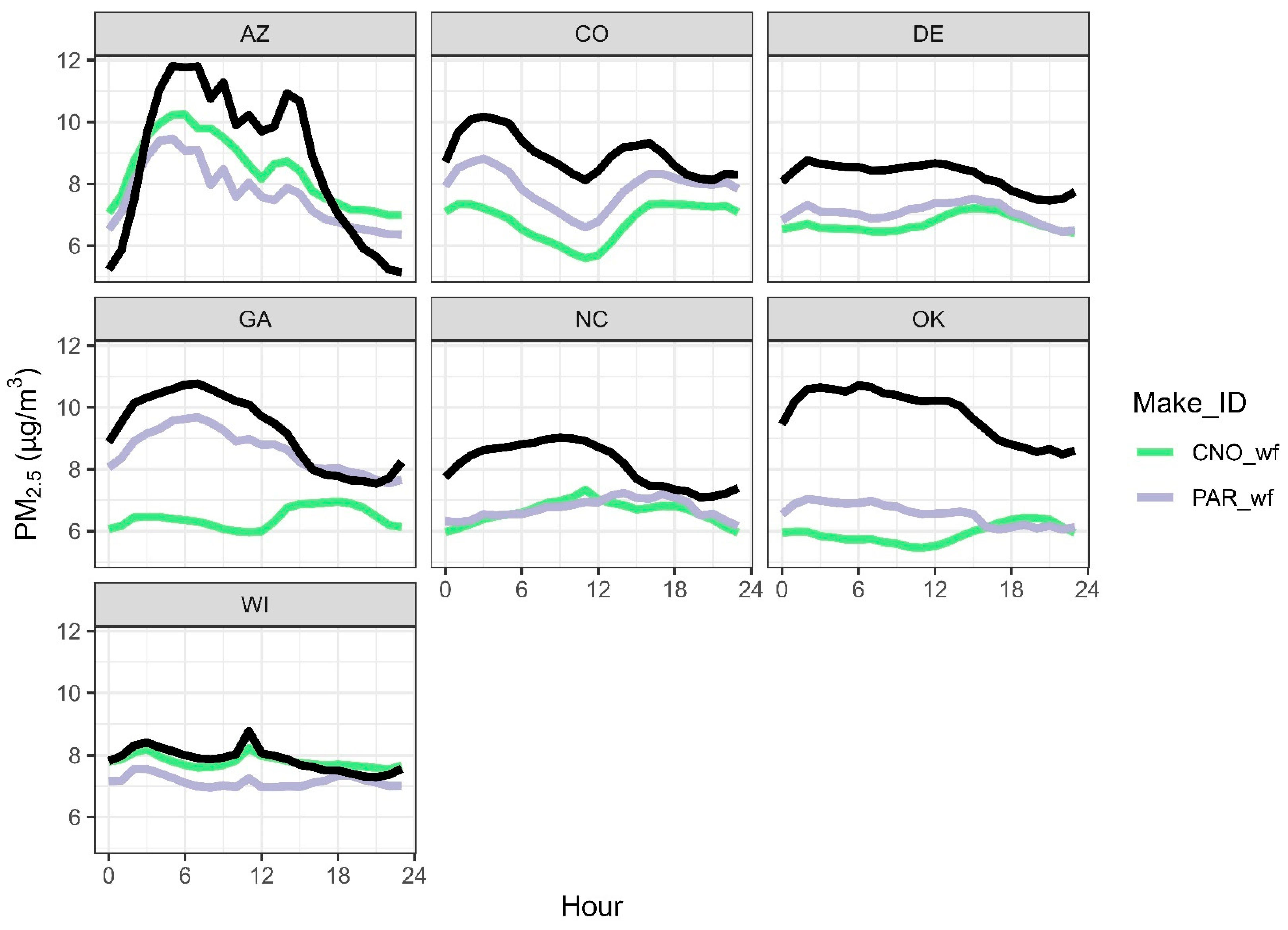
3.5.2. Hour of Day Performance
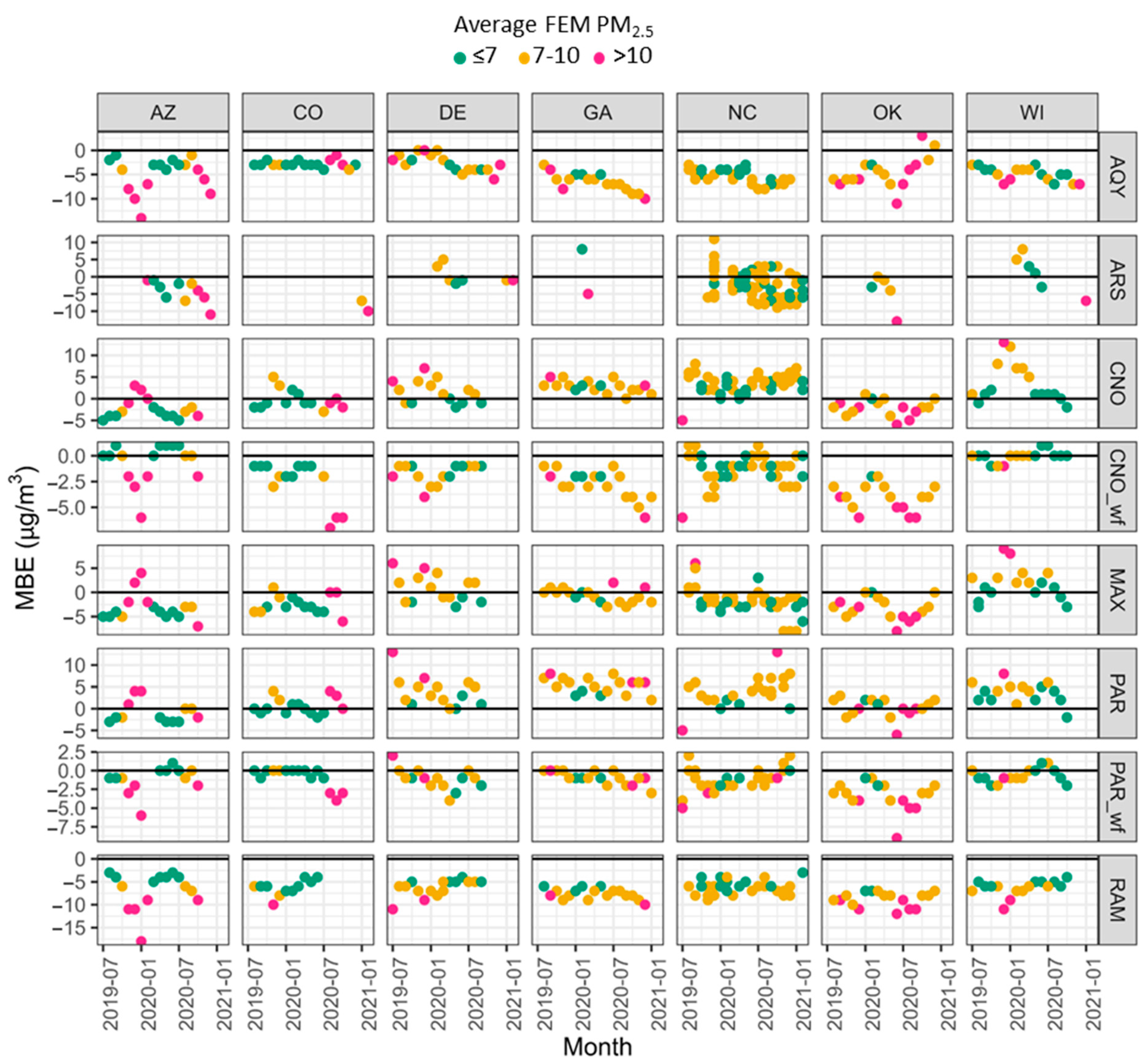
3.5.3. Monthly Bias
4. Conclusions
Supplementary Materials
Author Contributions
Funding
Data Availability Statement
Acknowledgments
Conflicts of Interest
Abbreviations
| AIRS | Air Innovation Research Site |
| AQY | Aeroqual AQY sensor |
| ARS | Arisense sensor |
| AZ | Arizona |
| CNO | Clarity Node and Clarity Node-S sensor |
| CNO_wf | Clarity Node sensor wildfire corrected |
| CO | Colorado |
| DE | Delaware |
| EPA | Environmental Protection Agency |
| GA | Georgia |
| NC | North Carolina |
| MAX | Maxima sensor |
| MBE | Mean bias error |
| MDPI | Multidisciplinary Digital Publishing Institute |
| OK | Oklahoma |
| O3 | Ozone |
| PAR | PurpleAir sensor |
| PAR_wf | PurpleAir sensor wildfire corrected |
| PM2.5 | Fine particulate matter |
| RAM | RAMP sensor |
| RH | Relative Humidity |
| WI | Wisconsin |
References
- Barkjohn, K.K.; Clements, A.; Mocka, C.; Barrette, C.; Bittner, A.; Champion, W.; Gantt, B.; Good, E.; Holder, A.; Hillis, B.; et al. Air Quality Sensor Experts Convene: Current Quality Assurance Considerations for Credible Data. ACS EST Air 2024, 1, 1203–1214. [Google Scholar] [CrossRef] [PubMed]
- Karagulian, F.; Barbiere, M.; Kotsev, A.; Spinelle, L.; Gerboles, M.; Lagler, F.; Redon, N.; Crunaire, S.; Borowiak, A. Review of the Performance of Low-Cost Sensors for Air Quality Monitoring. Atmosphere 2019, 10, 506. [Google Scholar] [CrossRef]
- Clements, A.L.; Reece, S.; Conner, T.; Williams, R. Observed data quality concerns involving low-cost air sensors. Atmos. Environ. X 2019, 3, 100034. [Google Scholar] [CrossRef] [PubMed]
- Kang, Y.; Aye, L.; Ngo, T.D.; Zhou, J. Performance evaluation of low-cost air quality sensors: A review. Sci. Total Environ. 2022, 818, 151769. [Google Scholar] [CrossRef] [PubMed]
- Giordano, M.R.; Malings, C.; Pandis, S.N.; Presto, A.A.; McNeill, V.F.; Westervelt, D.M.; Beekmann, M.; Subramanian, R. From low-cost sensors to high-quality data: A summary of challenges and best practices for effectively calibrating low-cost particulate matter mass sensors. J. Aerosol Sci. 2021, 158, 105833. [Google Scholar] [CrossRef]
- Duvall, R.M.; Hagler, G.S.W.; Clements, A.L.; Benedict, K.; Barkjohn, K.; Kilaru, V.; Hanley, T.; Watkins, N.; Kaufman, A.; Kamal, A.; et al. Deliberating Performance Targets: Follow-on workshop discussing PM10, NO2, CO, and SO2 air sensor targets. Atmos. Environ. 2020, 246, 118099. [Google Scholar] [CrossRef]
- Williams, R.; Duvall, R.; Kilaru, V.; Hagler, G.; Hassinger, L.; Benedict, K.; Rice, J.; Kaufman, A.; Judge, R.; Pierce, G.; et al. Deliberating performance targets workshop: Potential paths for emerging PM2.5 and O3 air sensor progress. Atmos. Environ. X 2019, 2, 100031. [Google Scholar] [CrossRef]
- Duvall, R.; Clements, A.; Barkjohn, K.; Kumar, M.; Greene, D.; Dye, T.; Papapostolou, V.; Mui, W.; Kuang, M. NO2, CO, and SO2 Supplement to the 2021 Report on Performance Testing Protocols, Metrics, and Target Values for Ozone Air Sensors; U.S. Environmental Protection Agency, Ed.; U.S. Environmental Protection Agency: Washington, DC, USA, 2024.
- Duvall, R.; Clements, A.; Barkjohn, K.; Kumar, M.; Greene, D.; Dye, T.; Papapostolou, V.; Mui, W.; Kuang, M. PM10 Supplement to the 2021 Report on Performance Testing Protocols, Metrics, and Target Values for Fine Particulate Matter Air Sensors; U.S. Environmental Protection Agency, Ed.; U.S. Environmental Protection Agency: Washington, DC, USA, 2023.
- Duvall, R.; Clements, A.; Hagler, G.; Kamal, A.; Kilaru, V.; Goodman, L.; Frederick, S.; Johnson Barkjohn, K.; VonWald, I.; Greene, D.; et al. Performance Testing Protocols, Metrics, and Target Values for Fine Particulate Matter Air Sensors: Use in Ambient, Outdoor, Fixed Site, Non-Regulatory Supplemental and Informational Monitoring Applications; EPA/600/R-20/280; U.S. Environmental Protection Agency, Office of Research and Development: Washington, DC, USA, 2021.
- Duvall, R.M.; Clements, A.L.; Hagler, G.; Kamal, A.; Kilaru, V.; Goodman, L.; Frederick, S.; Barkjohn, K.K.J.; VonWald, I.; Greene, D.; et al. Performance Testing Protocols, Metrics, and Target Values for Ozone Air Sensors: Use in Ambient, Outdoor, Fixed Site, Non-Regulatory Supplemental and Informational Monitoring Applications; EPA/600/R-20/279; U.S. Environmental Protection Agency: Washington, DC, USA, 2021.
- Feenstra, B.; Papapostolou, V.; Hasheminassab, S.; Zhang, H.; Boghossian, B.D.; Cocker, D.; Polidori, A. Performance evaluation of twelve low-cost PM2.5 sensors at an ambient air monitoring site. Atmos. Environ. 2019, 216, 116946. [Google Scholar] [CrossRef]
- Jiao, W.; Hagler, G.; Williams, R.; Sharpe, R.; Brown, R.; Garver, D.; Judge, R.; Caudill, M.; Rickard, J.; Davis, M.; et al. Community Air Sensor Network (CAIRSENSE) project: Evaluation of low-cost sensor performance in a suburban environment in the southeastern United States. Atmos. Meas. Tech. 2016, 9, 5281–5292. [Google Scholar] [CrossRef]
- Nilson, B.; Jackson, P.L.; Schiller, C.L.; Parsons, M.T. Development and Evaluation of Correction Models for a Low-Cost Fine Particulate Matter Monitor. Atmos. Meas. Tech. Discuss. 2022, 2022, 1–16. [Google Scholar] [CrossRef]
- Barkjohn, K.K.; Holder, A.L.; Frederick, S.G.; Clements, A.L. Correction and Accuracy of PurpleAir PM2.5 Measurements for Extreme Wildfire Smoke. Sensors 2022, 22, 9669. [Google Scholar] [CrossRef] [PubMed]
- Zheng, T.; Bergin, M.H.; Johnson, K.K.; Tripathi, S.N.; Shirodkar, S.; Landis, M.S.; Sutaria, R.; Carlson, D.E. Field evaluation of low-cost particulate matter sensors in high-and low-concentration environments. Atmos. Meas. Tech. 2018, 11, 4823–4846. [Google Scholar] [CrossRef]
- Johnson, K.K.; Bergin, M.H.; Russell, A.G.; Hagler, G.S. Field test of several low-cost particulate matter sensors in high and low concentration urban environments. Aerosol Air Qual. Res 2018, 18, 565–578. [Google Scholar] [CrossRef] [PubMed]
- Wallace, L.; Zhao, T.; Klepeis, N.E. Calibration of PurpleAir PA-I and PA-II Monitors Using Daily Mean PM2.5 Concentrations Measured in California, Washington, and Oregon from 2017 to 2021. Sensors 2022, 22, 4741. [Google Scholar] [CrossRef]
- deSouza, P.N.; Barkjohn, K.; Clements, A.; Lee, J.; Kahn, R.; Crawford, B.; Kinney, P. An analysis of degradation in low-cost particulate matter sensors. Environ. Sci. Atmos. 2023, 3, 521–536. [Google Scholar] [CrossRef]
- Karl, T.R.; Koss, W.J. Regional and National Monthly, Seasonal, and Annual Temperature Weighted by Area, 1895–1983. Hist. Climatol. Ser. 1984, 4-3, 38. [Google Scholar]
- NOAA. U.S. Climate Regions. Available online: https://www.ncdc.noaa.gov/monitoring-references/maps/us-climate-regions.php (accessed on 5 February 2025).
- Barkjohn, K.K.; Gantt, B.; Clements, A.L. Development and application of a United States-wide correction for PM2.5 data collected with the PurpleAir sensor. Atmos. Meas. Tech. 2021, 14, 4617–4637. [Google Scholar] [CrossRef] [PubMed]
- Jaffe, D.A.; Miller, C.; Thompson, K.; Finley, B.; Nelson, M.; Ouimette, J.; Andrews, E. An evaluation of the U.S. EPA’s correction equation for PurpleAir sensor data in smoke, dust, and wintertime urban pollution events. Atmos. Meas. Tech. 2023, 16, 1311–1322. [Google Scholar] [CrossRef]
- Ouimette, J.; Arnott, W.P.; Laven, P.; Whitwell, R.; Radhakrishnan, N.; Dhaniyala, S.; Sandink, M.; Tryner, J.; Volckens, J. Fundamentals of low-cost aerosol sensor design and operation. Aerosol Sci. Technol. 2023, 58, 1–15. [Google Scholar] [CrossRef]
- Ouimette, J.R.; Malm, W.C.; Schichtel, B.A.; Sheridan, P.J.; Andrews, E.; Ogren, J.A.; Arnott, W.P. Evaluating the PurpleAir monitor as an aerosol light scattering instrument. Atmos. Meas. Tech. 2022, 15, 655–676. [Google Scholar] [CrossRef]
- Kuula, J.; Kuuluvainen, H.; Rönkkö, T.; Niemi, J.V.; Saukko, E.; Portin, H.; Aurela, M.; Saarikoski, S.; Rostedt, A.; Hillamo, R.; et al. Applicability of Optical and Diffusion Charging-Based Particulate Matter Sensors to Urban Air Quality Measurements. Aerosol Air Qual. Res. 2019, 19, 1024–1039. [Google Scholar] [CrossRef]
- Kaur, K.; Kelly, K.E. Performance evaluation of the Alphasense OPC-N3 and Plantower PMS5003 sensor in measuring dust events in the Salt Lake Valley, Utah. Atmos. Meas. Tech. 2023, 16, 2455–2470. [Google Scholar] [CrossRef]
- Pope, R.; Stanley, K.M.; Domsky, I.; Yip, F.; Nohre, L.; Mirabelli, M.C. The relationship of high PM2.5 days and subsequent asthma-related hospital encounters during the fireplace season in Phoenix, AZ, 2008–2012. Air Qual. Atmos. Health 2017, 10, 161–169. [Google Scholar] [CrossRef]
- Li, Y.; Yuan, Z.; Chen, L.W.A.; Pillarisetti, A.; Yadav, V.; Wu, M.; Cui, H.; Zhao, C. From air quality sensors to sensor networks: Things we need to learn. Sens. Actuators B Chem. 2022, 351, 130958. [Google Scholar] [CrossRef]
- Aberkane, T. Evaluation of PM instruments in New Zealand. Air Qual. Clim. Change 2021, 55, 47–52. [Google Scholar]
- Toner, S.M. Evaluation of an optical PM measurement method compared to conventional PM measurement methods. Air Qual. Clim. Change 2021, 55, 63–70. [Google Scholar]
- Feinberg, S.; Williams, R.; Hagler, G.S.W.; Rickard, J.; Brown, R.; Garver, D.; Harshfield, G.; Stauffer, P.; Mattson, E.; Judge, R.; et al. Long-term evaluation of air sensor technology under ambient conditions in Denver, Colorado. Atmos. Meas. Tech. 2018, 11, 4605–4615. [Google Scholar] [CrossRef]
- Hagan, D.H.; Kroll, J.H. Assessing the accuracy of low-cost optical particle sensors using a physics-based approach. Atmos. Meas. Tech. 2020, 13, 6343–6355. [Google Scholar] [CrossRef] [PubMed]
- Ryder, O.S.; DeWinter, J.L.; Brown, S.G.; Hoffman, K.; Frey, B.; Mirzakhalili, A. Assessment of particulate toxic metals at an Environmental Justice community. Atmos. Environ. X 2020, 6, 100070. [Google Scholar] [CrossRef]
- Brown, S.G.; Penfold, B.; Mukherjee, A.; Landsberg, K.; Eisinger, D.S. Conditions Leading to Elevated PM2.5 at Near-Road Monitoring Sites: Case Studies in Denver and Indianapolis. Int. J. Environ. Res. Public Health 2019, 16, 1634. [Google Scholar] [CrossRef] [PubMed]
- Valerino, M.J.; Johnson, J.J.; Izumi, J.; Orozco, D.; Hoff, R.M.; Delgado, R.; Hennigan, C.J. Sources and composition of PM2.5 in the Colorado Front Range during the DISCOVER-AQ study. J. Geophys. Res. Atmos. 2017, 122, 566–582. [Google Scholar] [CrossRef]
- Upadhyay, N.; Clements, A.; Fraser, M.; Herckes, P. Chemical Speciation of PM2.5 and PM10 in South Phoenix, AZ. J. Air Waste Manag. Assoc. 2011, 61, 302–310. [Google Scholar] [CrossRef]
- Heo, J.; McGinnis, J.E.; de Foy, B.; Schauer, J.J. Identification of potential source areas for elevated PM2.5, nitrate and sulfate concentrations. Atmos. Environ. 2013, 71, 187–197. [Google Scholar] [CrossRef]
- Dreyfus, M.A.; Adou, K.; Zucker, S.M.; Johnston, M.V. Organic aerosol source apportionment from highly time-resolved molecular composition measurements. Atmos. Environ. 2009, 43, 2901–2910. [Google Scholar] [CrossRef]
- Stanier, C.; Singh, A.; Adamski, W.; Baek, J.; Caughey, M.; Carmichael, G.; Edgerton, E.; Kenski, D.; Koerber, M.; Oleson, J.; et al. Overview of the LADCO winter nitrate study: Hourly ammonia, nitric acid and PM2.5 composition at an urban and rural site pair during PM2.5 episodes in the US Great Lakes region. Atmos. Chem. Phys. 2012, 12, 11037–11056. [Google Scholar] [CrossRef]
- Clements, N.; Hannigan, M.P.; Miller, S.L.; Peel, J.L.; Milford, J.B. Comparisons of urban and rural PM10 − 2.5 and PM2.5 mass concentrations and semi-volatile fractions in northeastern Colorado. Atmos. Chem. Phys. 2016, 16, 7469–7484. [Google Scholar] [CrossRef]
- Weber, R. Short-Term Temporal Variation in PM2.5 Mass and Chemical Composition during the Atlanta Supersite Experiment, 1999. J. Air Waste Manag. Assoc. 2003, 53, 84–91. [Google Scholar] [CrossRef] [PubMed]
- Dutton, S.J.; Rajagopalan, B.; Vedal, S.; Hannigan, M.P. Temporal patterns in daily measurements of inorganic and organic speciated PM2.5 in Denver. Atmos. Environ. 2010, 44, 987–998. [Google Scholar] [CrossRef]
- Kerr, S.C.; Schauer, J.J.; Rodger, B. Regional haze in Wisconsin: Sources and the spatial distribution. J. Environ. Eng. Sci. 2004, 3, 213–222. [Google Scholar] [CrossRef]
- Petters, M.D.; Kreidenweis, S.M. A single parameter representation of hygroscopic growth and cloud condensation nucleus activity. Atmos. Chem. Phys. 2007, 7, 1961–1971. [Google Scholar] [CrossRef]
- Chan, E.A.W.; Gantt, B.; McDow, S. The reduction of summer sulfate and switch from summertime to wintertime PM2.5 concentration maxima in the United States. Atmos. Environ. 2018, 175, 25–32. [Google Scholar] [CrossRef] [PubMed]
- Zhai, X.; Mulholland, J.A.; Russell, A.G.; Holmes, H.A. Spatial and temporal source apportionment of PM2.5 in Georgia, 2002 to 2013. Atmos. Environ. 2017, 161, 112–121. [Google Scholar] [CrossRef]
- Bravo, M.A.; Warren, J.L.; Leong, M.C.; Deziel, N.C.; Kimbro, R.T.; Bell, M.L.; Miranda, M.L. Where Is Air Quality Improving, and Who Benefits? A Study of PM2.5 and Ozone over 15 Years. Am. J. Epidemiol. 2022, 191, 1258–1269. [Google Scholar] [CrossRef] [PubMed]
- He, J.; Harkins, C.; O’Dell, K.; Li, M.; Francoeur, C.; Aikin, K.C.; Anenberg, S.; Baker, B.; Brown, S.S.; Coggon, M.M.; et al. COVID-19 perturbation on US air quality and human health impact assessment. PNAS Nexus 2024, 3, pgad483. [Google Scholar] [CrossRef] [PubMed]
- Prakash, J.; Choudhary, S.; Raliya, R.; Chadha, T.S.; Fang, J.; George, M.P.; Biswas, P. Deployment of networked low-cost sensors and comparison to real-time stationary monitors in New Delhi. J. Air Waste Manag. Assoc. 2021, 71, 1347–1360. [Google Scholar] [CrossRef] [PubMed]
- Prakash, J.; Choudhary, S.; Raliya, R.; Chadha, T.; Fang, J.; Biswas, P. PM sensors as an indicator of overall air quality: Pre-COVID and COVID periods. Atmos. Pollut. Res. 2022, 13, 101594. [Google Scholar] [CrossRef] [PubMed]
- Dharaiya, V.R.; Malyan, V.; Kumar, V.; Sahu, M.; Venkatraman, C.; Biswas, P.; Yadav, K.; Haswani, D.; Raman, R.S.; Bhat, R.; et al. Evaluating the Performance of Low-cost PM Sensors over Multiple COALESCE Network Sites. Aerosol Air Qual. Res. 2023, 23, 220390. [Google Scholar] [CrossRef]
- Edwards, L.; Rutter, G.; Iverson, L.; Wilson, L.; Chadha, T.S.; Wilkinson, P.; Milojevic, A. Personal exposure monitoring of PM2.5 among US diplomats in Kathmandu during the COVID-19 lockdown, March to June 2020. Sci. Total Environ. 2021, 772, 144836. [Google Scholar] [CrossRef]
- Prajapati, B.; Dharaiya, V.; Sahu, M.; Venkatraman, C.; Biswas, P.; Yadav, K.; Pullokaran, D.; Raman, R.S.; Bhat, R.; Najar, T.A.; et al. Development of a physics-based method for calibration of low-cost particulate matter sensors and comparison with machine learning models. J. Aerosol Sci. 2024, 175, 106284. [Google Scholar] [CrossRef]
- Malyan, V.; Kumar, V.; Sahu, M.; Prakash, J.; Choudhary, S.; Raliya, R.; Chadha, T.S.; Fang, J.; Biswas, P. Calibrating low-cost sensors using MERRA-2 reconstructed PM2.5 mass concentration as a proxy. Atmos. Pollut. Res. 2024, 15, 102027. [Google Scholar] [CrossRef]
- Li, J.Y.; Mattewal, S.K.; Patel, S.; Biswas, P. Evaluation of Nine Low-cost-sensor-based Particulate Matter Monitors. Aerosol Air Qual. Res. 2020, 20, 254–270. [Google Scholar] [CrossRef]
- Vidwans, A.; Choudhary, S.; Jolliff, B.; Gillis-Davis, J.; Biswas, P. Size and charge distribution characteristics of fine and ultrafine particles in simulated lunar dust: Relevance to lunar missions and exploration. Planet. Space Sci. 2022, 210, 105392. [Google Scholar] [CrossRef]
- Do, K.; Yu, H.; Velasquez, J.; Grell-Brisk, M.; Smith, H.; Ivey, C.E. A data-driven approach for characterizing community scale air pollution exposure disparities in inland Southern California. J. Aerosol Sci. 2021, 152, 105704. [Google Scholar] [CrossRef]
- Coker, E.S.; Amegah, A.K.; Mwebaze, E.; Ssematimba, J.; Bainomugisha, E. A land use regression model using machine learning and locally developed low cost particulate matter sensors in Uganda. Environ. Res. 2021, 199, 111352. [Google Scholar] [CrossRef] [PubMed]
- Njeru, M.N.; Mwangi, E.; Gatari, M.J.; Kaniu, M.I.; Kanyeria, J.; Raheja, G.; Westervelt, D.M. First Results From a Calibrated Network of Low-Cost PM2.5 Monitors in Mombasa, Kenya Show Exceedance of Healthy Guidelines. GeoHealth 2024, 8, e2024GH001049. [Google Scholar] [CrossRef]
- Raheja, G.; Nimo, J.; Appoh, E.K.E.; Essien, B.; Sunu, M.; Nyante, J.; Amegah, M.; Quansah, R.; Arku, R.E.; Penn, S.L.; et al. Low-Cost Sensor Performance Intercomparison, Correction Factor Development, and 2+ Years of Ambient PM2.5 Monitoring in Accra, Ghana. Environ. Sci. Technol. 2023, 57, 10708–10720. [Google Scholar] [CrossRef] [PubMed]
- Holder, A.L.; Mebust, A.K.; Maghran, L.A.; McGown, M.R.; Stewart, K.E.; Vallano, D.M.; Elleman, R.A.; Baker, K.R. Field Evaluation of Low-Cost Particulate Matter Sensors for Measuring Wildfire Smoke. Sensors 2020, 20, 4796. [Google Scholar] [CrossRef]
- Weissert, L.F.; Henshaw, G.S.; Clements, A.L.; Duvall, R.M.; Croghan, C. Seasonal effects in the application of the MOMA remote calibration tool to outdoor PM2.5 air sensors. EGUsphere 2024, 2024, 1–18. [Google Scholar]
- Bittner, A.S.; Cross, E.S.; Hagan, D.H.; Malings, C.; Lipsky, E.; Grieshop, A.P. Performance characterization of low-cost air quality sensors for off-grid deployment in rural Malawi. Atmos. Meas. Tech. 2022, 15, 3353–3376. [Google Scholar] [CrossRef]
- Weissert, L.F.; Henshaw, G.S.; Williams, D.E.; Feenstra, B.; Lam, R.; Collier-Oxandale, A.; Papapostolou, V.; Polidori, A. Performance evaluation of MOMA (MOment MAtching)—A remote network calibration technique for PM2.5 and PM10 sensors. Atmos. Meas. Tech. 2023, 16, 4709–4722. [Google Scholar] [CrossRef]
- Khreis, H.; Johnson, J.; Jack, K.; Dadashova, B.; Park, E.S. Evaluating the performance of low-cost air quality monitors in Dallas, Texas. Int. J. Environ. Res. Public Health 2022, 19, 1647. [Google Scholar] [CrossRef] [PubMed]
- Bahino, J.; Giordano, M.; Beekmann, M.; Yoboué, V.; Ochou, A.; Galy-Lacaux, C.; Liousse, C.; Hughes, A.; Nimo, J.; Lemmouchi, F.; et al. Temporal variability and regional influences of PM2.5 in the West African cities of Abidjan (Côte d’Ivoire) and Accra (Ghana). Environ. Sci. Atmos. 2024, 4, 468–487. [Google Scholar] [CrossRef]
- Malings, C.; Tanzer, R.; Hauryliuk, A.; Saha, P.K.; Robinson, A.L.; Presto, A.A.; Subramanian, R. Fine particle mass monitoring with low-cost sensors: Corrections and long-term performance evaluation. Aerosol Sci. Technol. 2019, 54, 160–174. [Google Scholar] [CrossRef]
- Wallace, L. Cracking the code—Matching a proprietary algorithm for a low-cost sensor measuring PM1 and PM2.5. Sci. Total Environ. 2023, 893, 164874. [Google Scholar] [CrossRef] [PubMed]
- Madhwal, S.; Tripathi, S.N.; Bergin, M.H.; Bhave, P.; de Foy, B.; Reddy, T.V.R.; Chaudhry, S.K.; Jain, V.; Garg, N.; Lalwani, P. Evaluation of PM2.5 spatio-temporal variability and hotspot formation using low-cost sensors across urban-rural landscape in lucknow, India. Atmos. Environ. 2024, 319, 120302. [Google Scholar] [CrossRef]
- Harr, L.; Sinsel, T.; Simon, H.; Esper, J. Seasonal Changes in Urban PM2.5 Hotspots and Sources from Low-Cost Sensors. Atmosphere 2022, 13, 694. [Google Scholar] [CrossRef]
- Francis, D.; Nelli, N.; Fonseca, R.; Weston, M.; Flamant, C.; Cherif, C. The dust load and radiative impact associated with the June 2020 historical Saharan dust storm. Atmos. Environ. 2022, 268, 118808. [Google Scholar] [CrossRef]
- Long, R.W.; Urbanski, S.P.; Lincoln, E.; Colon, M.; Kaushik, S.; Krug, J.D.; Vanderpool, R.W.; Landis, M.S. Summary of PM2.5 measurement artifacts associated with the Teledyne T640 PM Mass Monitor under controlled chamber experimental conditions using polydisperse ammonium sulfate aerosols and biomass smoke. J. Air Waste Manag. Assoc. 2023, 73, 295–312. [Google Scholar] [CrossRef]
- Hagler, G.; Hanley, T.; Hassett-Sipple, B.; Vanderpool, R.; Smith, M.; Wilbur, J.; Wilbur, T.; Oliver, T.; Shand, D.; Vidacek, V.; et al. Evaluation of two collocated federal equivalent method PM2.5 instruments over a wide range of concentrations in Sarajevo, Bosnia and Herzegovina. Atmos. Pollut. Res. 2022, 13, 101374. [Google Scholar] [CrossRef] [PubMed]
- O’Brien, E.; Torr, S. A comparison between a TAPI T640X, TEOM 1405-DF and reference samplers for the measurement of PM10 and PM2.5 at an urban location in Brisbane. Air Qual. Clim. Change 2021, 55, 71–76. [Google Scholar]
- Sandhu, T.; Robinson, M.C.; Rawlins, E.; Ardon-Dryer, K. Identification of dust events in the greater Phoenix area. Atmos. Pollut. Res. 2024, 15, 102275. [Google Scholar] [CrossRef]


| Number Evaluated | |||||||||
|---|---|---|---|---|---|---|---|---|---|
| ID | Make | Model | Internal PM Sensor | Communication | Power Source | NC | Other Sites | Measured Pollutants | Sampling Interval |
| AQY | Aeroqual (Auckland, New Zealand) | AQY * | Nova SDS011 | Cellular Wi-Fi (NC only) | Wall | 3 | 6 | PM2.5, NO2, O3, T, RH | 1 min |
| CNO | Clarity Movement Co. (Berkeley, CA, USA) | Node * | Plantower PMS6003 | Cellular | Wall | - | 6 | PM2.5, NO2 *, T, RH | ~5 min (Node) ~15 min (Node-S, NC only) |
| Node-S | Wi-Fi | Solar | 3 | - | PM2.5, NO2 *, T, RH | 30 s | |||
| MAX | Applied Particle Technology (Boise, ID, USA) | Maxima | Plantower PMSA003 | Wi-Fi | Wall | 3 | 6 | PM1, PM2.5, PM10, T, RH, P | 30 s |
| PAR | PurpleAir (Draper, UT, USA) | PA-II-SD * | Plantower PMS5003 (×2) | Wi-Fi | Wall | 3 | 6 | PM1, PM2.5, PM10, T, RH, P | 2 min |
| RAM | Sensit Technologies (Valparaiso, IN, USA) | RAMP | Plantower PMS5003 | Direct (no Wi-Fi/Cellular) | Wall | 3 | 6 | PM2.5, CO, NO, NO2, SO2, O3 | 15 s |
| ARS | Aerodyne ‡ (Billerica, MA, USA) | Arisense * | Particles Plus OPC | Cellular | Wall | 7 | 6 | PM1, PM2.5, PM10, CO, CO2, NO, NO2, O3, T, RH, P, WS, WD | 2 min |
| Location (City, State) | AQS ID | Monitor * | Spatial Scale | Site Type | Average Monitor PM2.5 | Maximum Hourly Monitor PM2.5 |
|---|---|---|---|---|---|---|
| (µg/m3) | (µg/m3) | |||||
| Phoenix, AZ, USA | 04-013-0019 | Thermo TEOM 1405-DF | Neighborhood | Population Exposure Highest Concentration | 8.9 | 550 |
| Denver, CO, USA | 08-031-0026 | Teledyne T640 | Neighborhood Urban | National Core Network (Ncore) State or Local Air Monitoring Stations (SLAMS) | 8.8 | 207 |
| Wilmington, DE, USA | 10-003-2004 | Teledyne T640 | Neighborhood | Population Exposure Maximum Concentration NCore Photochemical Assessment Monitoring Stations (PAMS) | 8.3 | 44 |
| Decatur, GA, USA | 13-089-0002 | Teledyne T640x | Neighborhood | Population Exposure Highest Concentration | 9.1 | 96 |
| Research Triangle Park, NC, USA | 37-063-0099 | Teledyne T640 | Neighborhood | NCore | 8.2 | 82 |
| Oklahoma City, OK, USA | 40-109-1037 | Teledyne T640 (until 31 December 2019) Teledyne T640x (starting 1 January 2020) | Urban Population Exposure | SLAMS | 10.0 | 110 |
| Milwaukee, WI, USA | 55-079-0026 | Teledyne T640x | Urban Neighborhood Population Exposure | SLAMS | 7.9 | 335 |
| Uncorrected PAR, CNO | |||||
|---|---|---|---|---|---|
| Make ID | Location | Range MBE | R2 | Range MBE | R2 |
| RAM | AZ | 15 | 0.88 | ||
| AQY | AZ | 13 | 0.64 | ||
| MAX | AZ | 11 | 0.92 | ||
| ARS | AZ | 10 | 0.45 | ||
| PAR_wf | AZ | 7 | 0.87 | 7 | 0.87 |
| CNO_wf | AZ | 7 | 0.88 | 8 | 0.91 |
| MAX | CO | 7 | 0.92 | ||
| RAM | CO | 6 | 0.35 | ||
| CNO_wf | CO | 6 | 0.93 | 8 | 0.79 |
| PAR_wf | CO | 4 | 0.94 | 6 | 0.93 |
| ARS | CO | 3 | 0.15 | ||
| AQY | CO | 3 | 0.82 | ||
| MAX | DE | 9 | 0.86 | ||
| ARS | DE | 7 | 0.45 | ||
| RAM | DE | 7 | 0.58 | ||
| AQY | DE | 6 | 0.75 | ||
| PAR_wf | DE | 6 | 0.84 | 13 | 0.86 |
| CNO_wf | DE | 3 | 0.81 | 9 | 0.84 |
| ARS | GA | 13 | 0.12 | ||
| AQY | GA | 7 | 0.42 | ||
| CNO_wf | GA | 5 | 0.57 | 5 | 0.77 |
| MAX | GA | 5 | 0.79 | ||
| RAM | GA | 4 | 0.64 | ||
| PAR_wf | GA | 3 | 0.75 | 6 | 0.78 |
| ARS | NC | 20 | 0.12 | ||
| MAX | NC | 14 | 0.67 | ||
| CNO_wf | NC | 7 | 0.6 | 13 | 0.61 |
| PAR_wf | NC | 7 | 0.76 | 18 | 0.77 |
| RAM | NC | 6 | 0.32 | ||
| AQY | NC | 5 | 0.41 | ||
| AQY | OK | 14 | 0.21 | ||
| ARS | OK | 13 | 0.42 | ||
| MAX | OK | 8 | 0.55 | ||
| PAR_wf | OK | 8 | 0.68 | 9 | 0.67 |
| RAM | OK | 5 | 0.38 | ||
| CNO_wf | OK | 4 | 0.71 | 7 | 0.68 |
| ARS | WI | 15 | 0.16 | ||
| MAX | WI | 12 | 0.9 | ||
| RAM | WI | 7 | 0.45 | ||
| AQY | WI | 4 | 0.75 | ||
| PAR_wf | WI | 3 | 0.83 | 10 | 0.81 |
| CNO_wf | WI | 2 | 0.88 | 15 | 0.83 |
Disclaimer/Publisher’s Note: The statements, opinions and data contained in all publications are solely those of the individual author(s) and contributor(s) and not of MDPI and/or the editor(s). MDPI and/or the editor(s) disclaim responsibility for any injury to people or property resulting from any ideas, methods, instructions or products referred to in the content. |
© 2025 by the authors. Licensee MDPI, Basel, Switzerland. This article is an open access article distributed under the terms and conditions of the Creative Commons Attribution (CC BY) license (https://creativecommons.org/licenses/by/4.0/).
Share and Cite
Barkjohn, K.K.; Yaga, R.; Thomas, B.; Schoppman, W.; Docherty, K.S.; Clements, A.L. Evaluation of Long-Term Performance of Six PM2.5 Sensor Types. Sensors 2025, 25, 1265. https://doi.org/10.3390/s25041265
Barkjohn KK, Yaga R, Thomas B, Schoppman W, Docherty KS, Clements AL. Evaluation of Long-Term Performance of Six PM2.5 Sensor Types. Sensors. 2025; 25(4):1265. https://doi.org/10.3390/s25041265
Chicago/Turabian StyleBarkjohn, Karoline K., Robert Yaga, Brittany Thomas, William Schoppman, Kenneth S. Docherty, and Andrea L. Clements. 2025. "Evaluation of Long-Term Performance of Six PM2.5 Sensor Types" Sensors 25, no. 4: 1265. https://doi.org/10.3390/s25041265
APA StyleBarkjohn, K. K., Yaga, R., Thomas, B., Schoppman, W., Docherty, K. S., & Clements, A. L. (2025). Evaluation of Long-Term Performance of Six PM2.5 Sensor Types. Sensors, 25(4), 1265. https://doi.org/10.3390/s25041265