
Enhanced Pure Pursuit Path Tracking Algorithm for Mobile Robots Optimized by NSGA-II with High-Precision GNSS Navigation

 , , , and
Abstract
1. Introduction
1.1. Mobile Robotics Applications
1.2. GNSS−Based Localization and Navigation
1.3. Comparative Analysis of Path Tracing Algorithms
1.4. Thesis Outline
2. Measurement Model Description
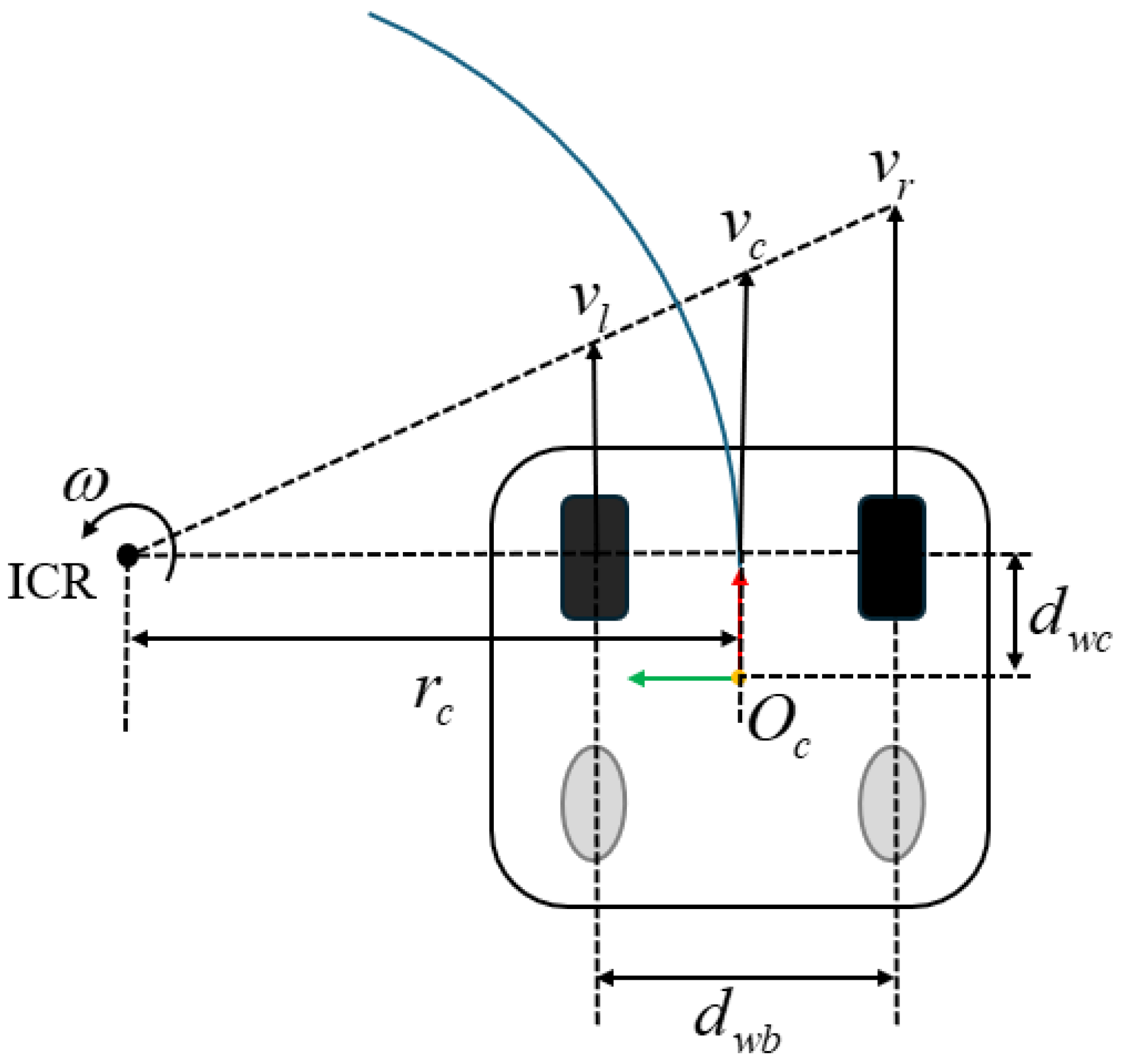
2.1. Rigid−Body Kinematic Model
2.2. IMU Measurement Model
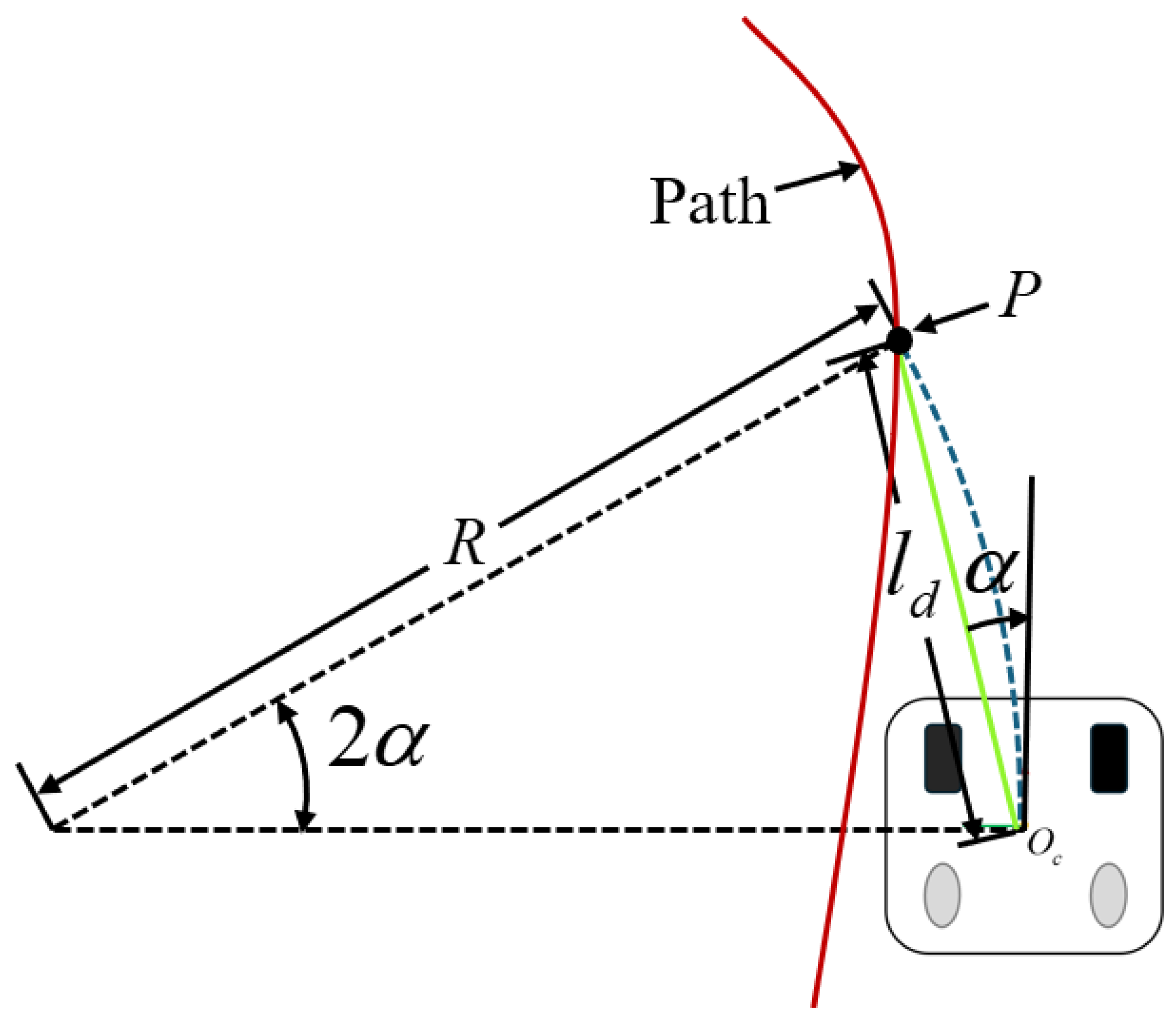
3. Enhancements of Pure Pursuit Tracking
3.1. Proposed Model with Integral Term for Lateral Error
3.2. Distance Convention and Global Path Generation
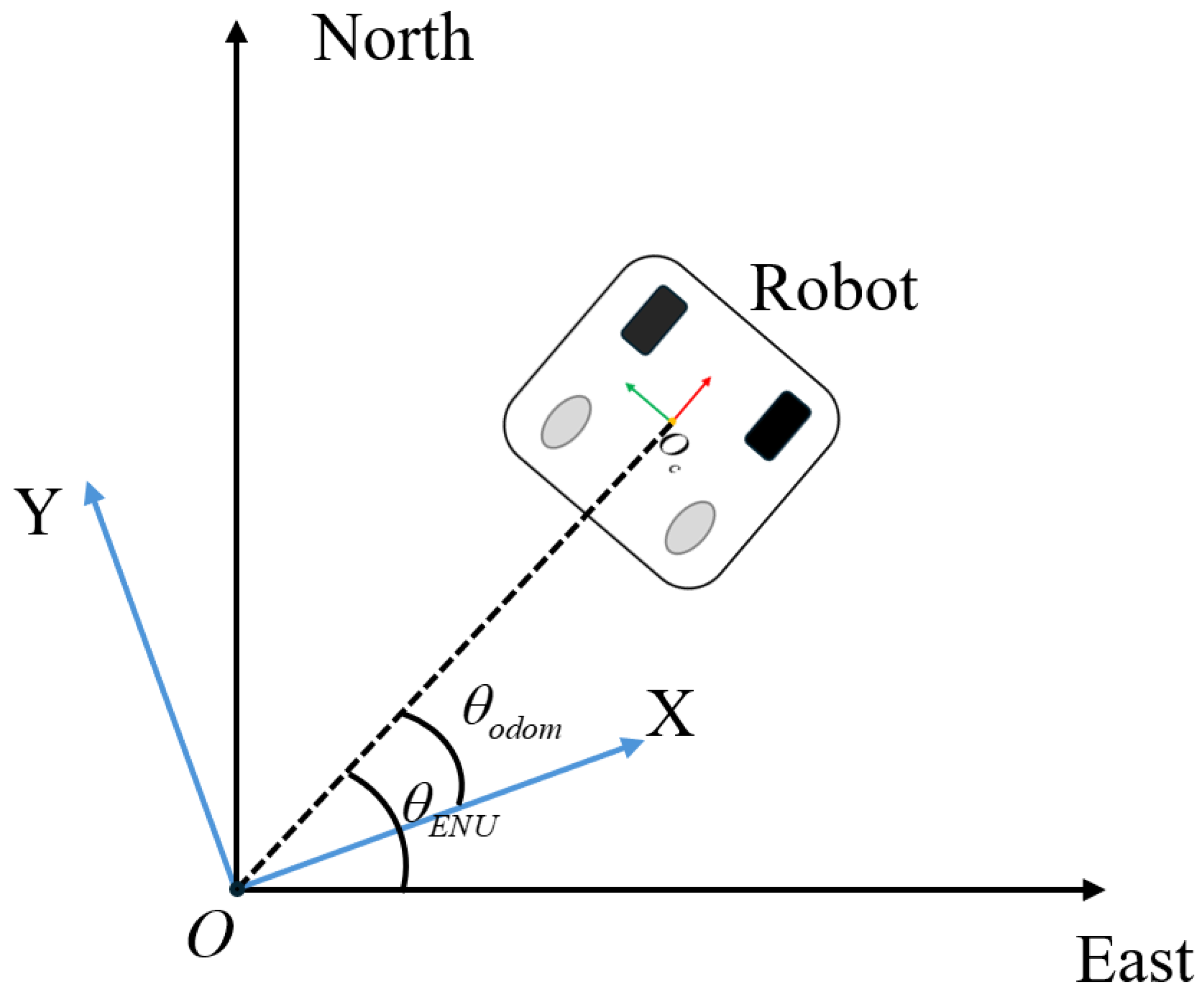
3.3. Coordinate Transformation
3.4. NSGA-II Objective Function Construction
3.5. Parameter Optimization and Logic Using NSGA-II Algorithm
| Algorithm 1 NSGA-II Algorithm Optimization for Path Following Control |
|
4. Results
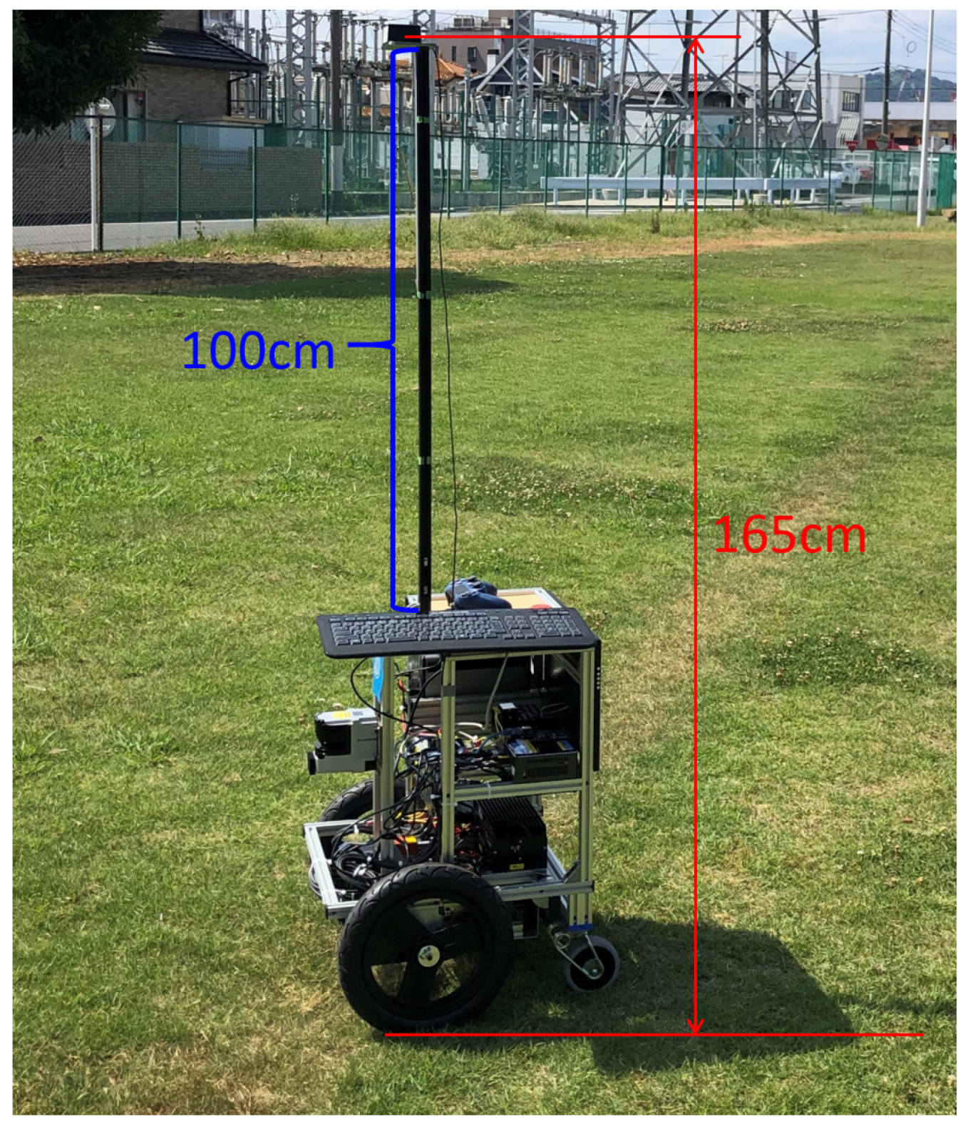
4.1. Robot Platform
- Baud rate: 115, 200.
- Data: 8 bit.
- Parity: none.
- Stop: 1 bit.
- Flow control: none.
4.2. GNSS Calibration
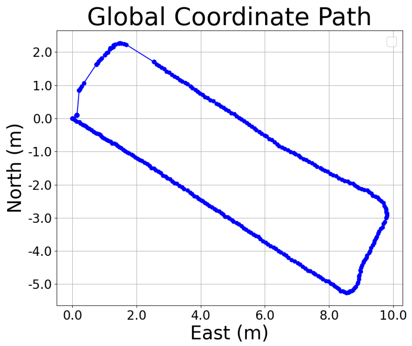
4.3. Path Generation
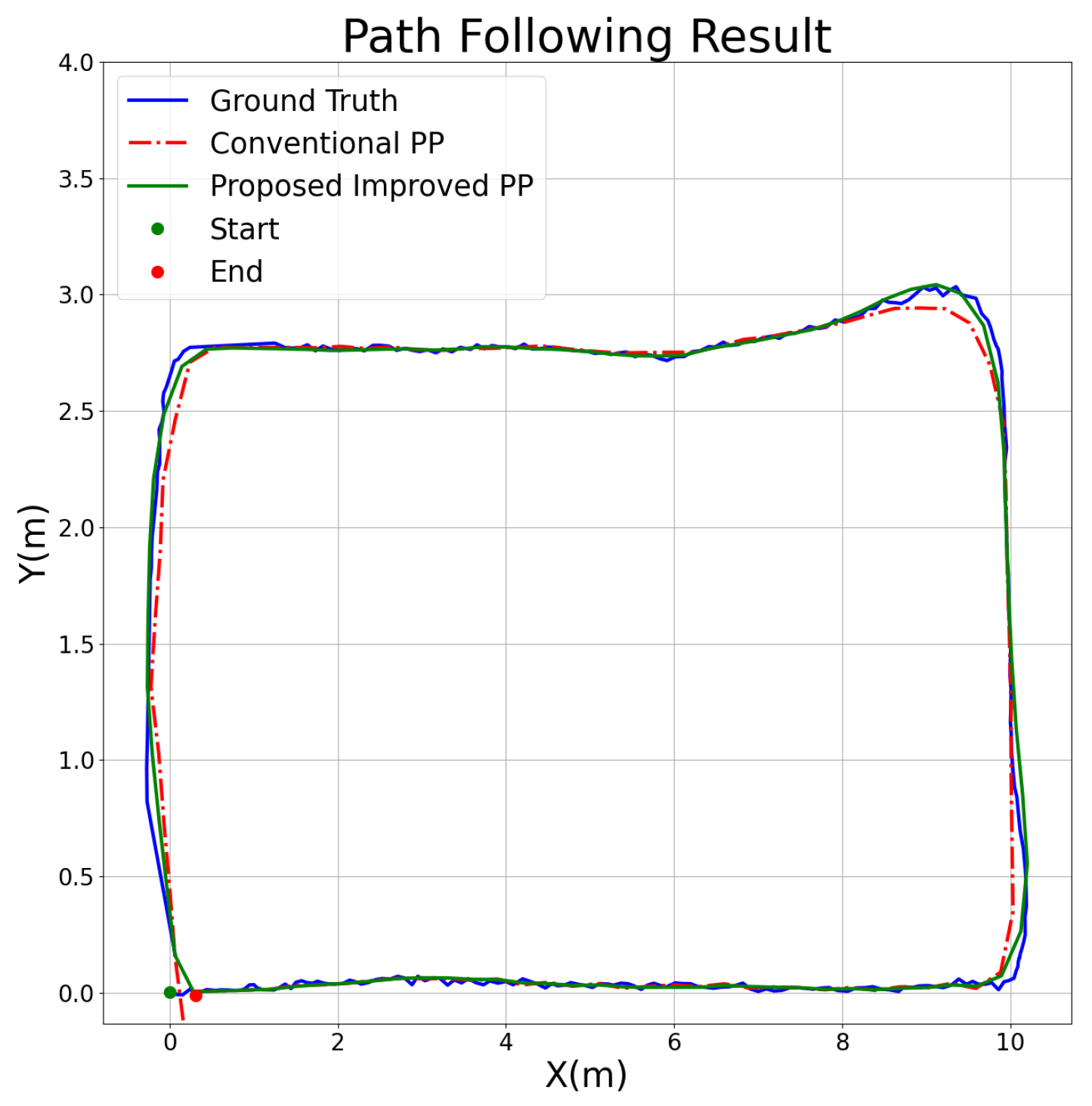
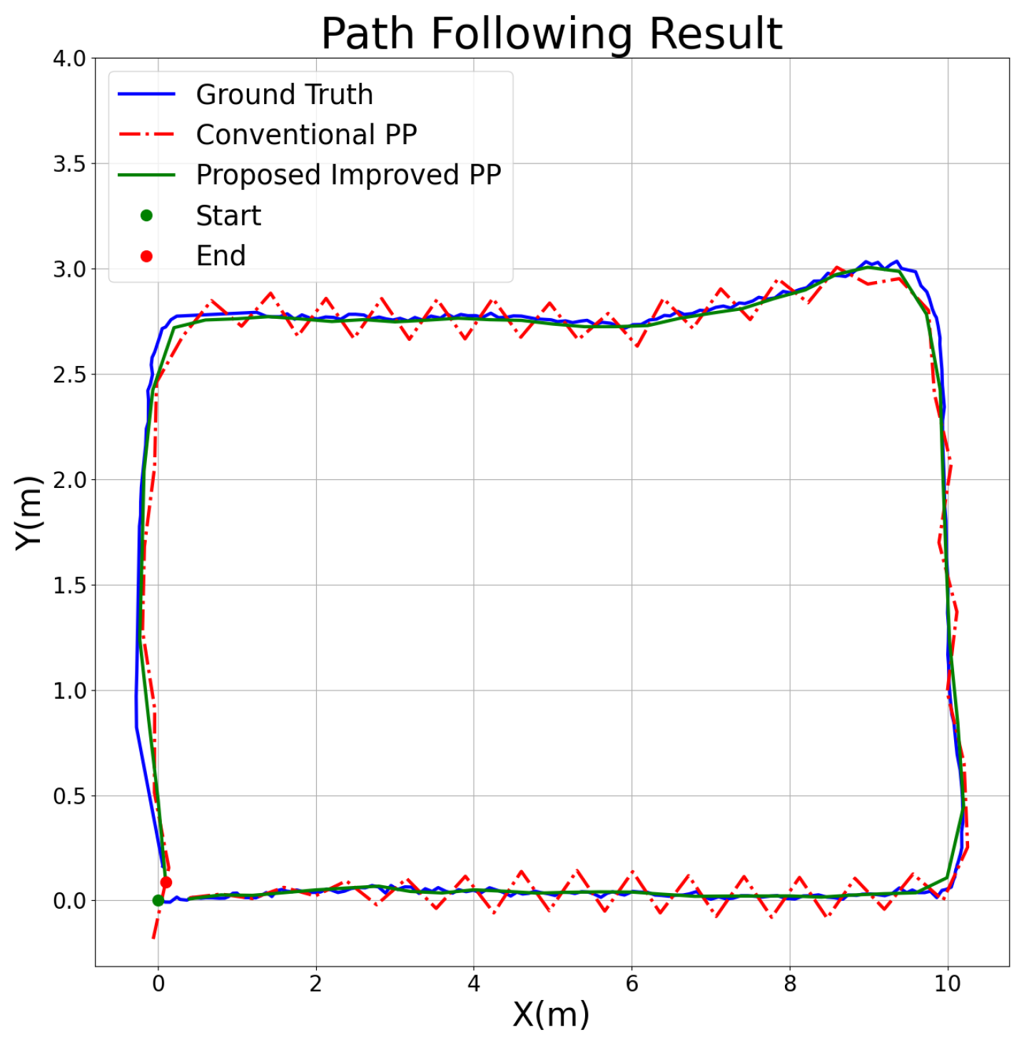
4.4. Path Following Result Analysis
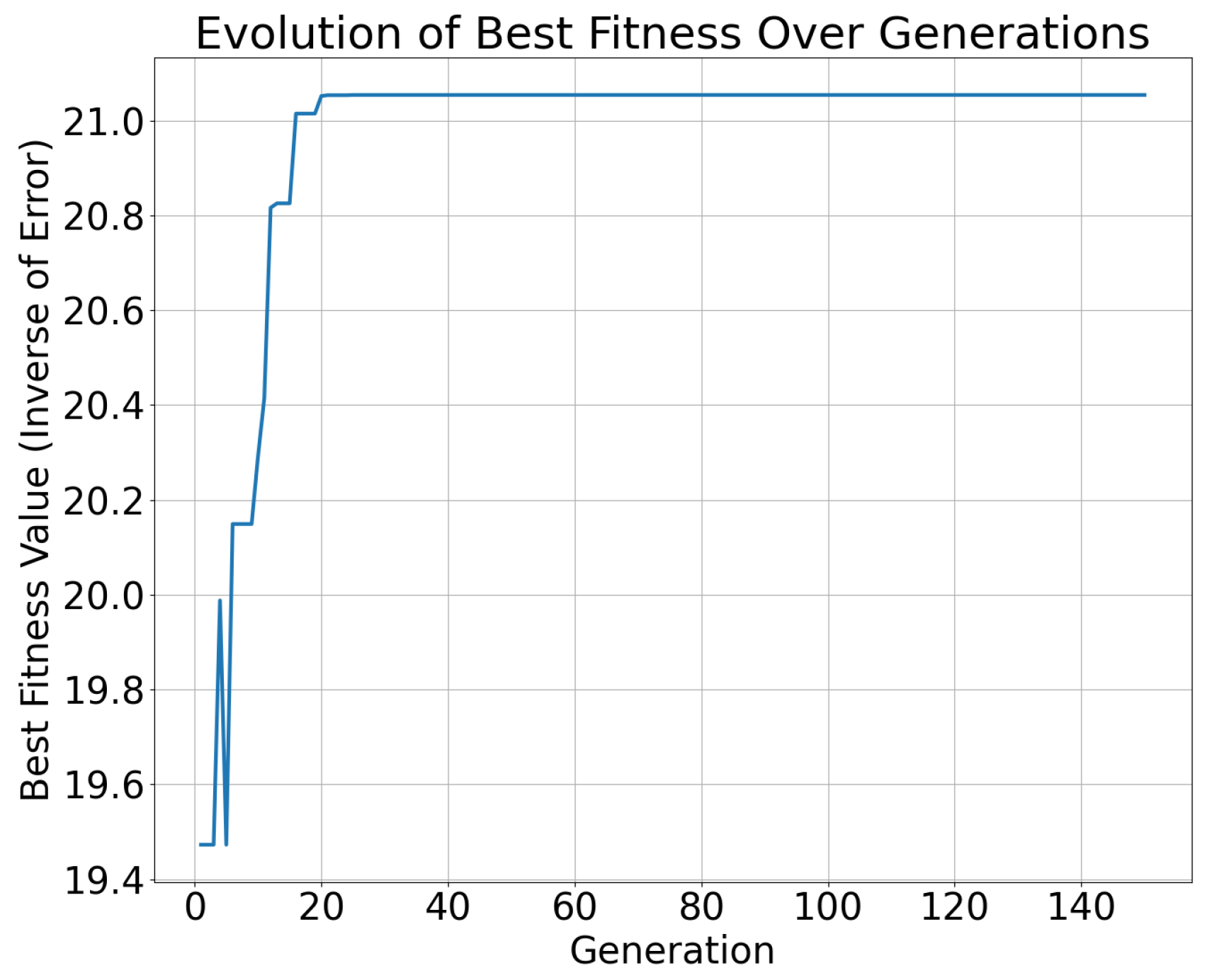
4.5. NSGA-II Iteration Result Analysis
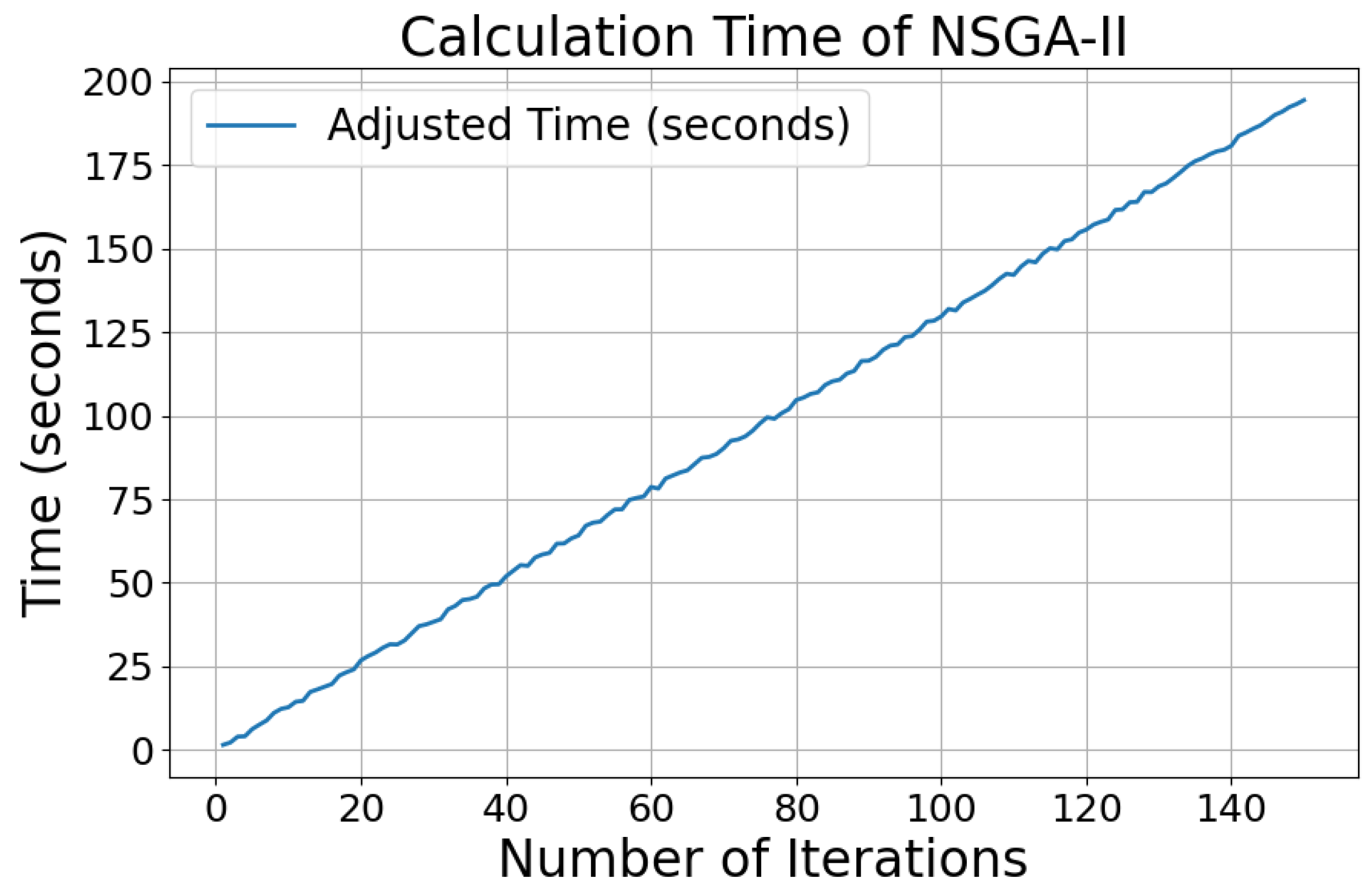
4.6. Real Time Performance Test and Analysis
5. Conclusions
6. Future Work
Author Contributions
Funding
Institutional Review Board Statement
Informed Consent Statement
Data Availability Statement
Conflicts of Interest
Abbreviations
| GNSS | Global Navigation Satellite System |
| INS | Inertial Navigation System |
| RTK | Real Time Kinematic |
| IMU | Inertial Measurement Unit |
| ODO | Odometer |
| LPS | Localization Positioning System |
| PI | Proportional Integral (Control) |
| APE | Absolute Pose Error |
| NSGA-II | Non−dominated Sorting Genetic Algorithm II |
| ENU | East−North−Up (Coordinate System) |
| LLA | Longitude, Latitude, Altitude (Coordinate System) |
References
- Raj, R.; Kos, A. A comprehensive study of mobile robot: History, developments, applications, and future research perspectives. Appl. Sci. 2022, 12, 6951. [Google Scholar] [CrossRef]
- Miclea, V.C.; Nedevschi, S. Monocular depth estimation with improved long-range accuracy for UAV environment perception. IEEE Trans. Geosci. Remote Sens. 2021, 60, 5602215. [Google Scholar] [CrossRef]
- Zhao, X.; Pu, F.; Wang, Z.; Chen, H.; Xu, Z. Detection, tracking, and geolocation of moving vehicle from uav using monocular camera. IEEE Access 2019, 7, 101160–101170. [Google Scholar] [CrossRef]
- Montanaro, U.; Dixit, S.; Fallah, S.; Dianati, M.; Stevens, A.; Oxtoby, D.; Mouzakitis, A. Towards connected autonomous driving: Review of use-cases. Veh. Syst. Dyn. 2019, 57, 779–814. [Google Scholar] [CrossRef]
- Parekh, D.; Poddar, N.; Rajpurkar, A.; Chahal, M.; Kumar, N.; Joshi, G.P.; Cho, W. A review on autonomous vehicles: Progress, methods and challenges. Electronics 2022, 11, 2162. [Google Scholar] [CrossRef]
- Li, J.; Wu, X.; Fan, J.; Liu, Y.; Xu, M. Overcoming driving challenges in complex urban traffic: A multi-objective eco-driving strategy via safety model based reinforcement learning. Energy 2023, 284, 128517. [Google Scholar] [CrossRef]
- Radočaj, D.; Plaščak, I.; Jurišić, M. Global navigation satellite systems as state-of-the-art solutions in precision agriculture: A review of studies indexed in the web of science. Agriculture 2023, 13, 1417. [Google Scholar] [CrossRef]
- Jin, S.; Wang, Q.; Dardanelli, G. A review on multi-GNSS for earth observation and emerging applications. Remote Sens. 2022, 14, 3930. [Google Scholar] [CrossRef]
- Guo, J.; Li, X.; Li, Z.; Hu, L.; Yang, G.; Zhao, C.; Fairbairn, D.; Watson, D.; Ge, M. Multi-GNSS precise point positioning for precision agriculture. Precis. Agric. 2018, 19, 895–911. [Google Scholar] [CrossRef]
- Sui, Y.; Yang, Z.; Zhuo, H.; You, Y.; Que, W.; He, N. A Fuzzy Pure Pursuit for Autonomous UGVs Based on Model Predictive Control and Whole-Body Motion Control. Drones 2024, 8, 554. [Google Scholar] [CrossRef]
- Sünderhauf, N.; Obst, M.; Wanielik, G.; Protzel, P. Multipath mitigation in GNSS-based localization using robust optimization. In Proceedings of the 2012 IEEE Intelligent Vehicles Symposium, Madrid, Spain, 3–7 June 2012; pp. 784–789. [Google Scholar]
- Hussain, A.; Akhtar, F.; Khand, Z.H.; Rajput, A.; Shaukat, Z. Complexity and limitations of GNSS signal reception in highly obstructed environments. Eng. Technol. Appl. Sci. Res. 2021, 11, 6864–6868. [Google Scholar] [CrossRef]
- Egea-Roca, D.; Arizabaleta-Diez, M.; Pany, T.; Antreich, F.; Lopez-Salcedo, J.A.; Paonni, M.; Seco-Granados, G. GNSS user technology: State-of-the-art and future trends. IEEE Access 2022, 10, 39939–39968. [Google Scholar] [CrossRef]
- Maier, D.; Kleiner, A. Improved GPS sensor model for mobile robots in urban terrain. In Proceedings of the 2010 IEEE International Conference on Robotics and Automation, Anchorage, AK, USA, 3–7 May 2010; pp. 4385–4390. [Google Scholar]
- Tao, Y.; Liu, C.; Liu, C.; Zhao, X.; Hu, H. Empirical wavelet transform method for GNSS coordinate series denoising. J. Geovisualization Spat. Anal. 2021, 5, 9. [Google Scholar] [CrossRef]
- Huang, G.; Du, S.; Wang, D. GNSS techniques for real-time monitoring of landslides: A review. Satell. Navig. 2023, 4, 5. [Google Scholar] [CrossRef]
- Fung, M.L.; Chen, M.Z.; Chen, Y.H. Sensor fusion: A review of methods and applications. In Proceedings of the 2017 29th Chinese Control And Decision Conference (CCDC), Chongqing, China, 28–30 May 2017; pp. 3853–3860. [Google Scholar]
- Sun, R.; Yang, Y.; Chiang, K.W.; Duong, T.T.; Lin, K.Y.; Tsai, G.J. Robust IMU/GPS/VO integration for vehicle navigation in GNSS degraded urban areas. IEEE Sens. J. 2020, 20, 10110–10122. [Google Scholar] [CrossRef]
- Samuel, M.; Hussein, M.; Mohamad, M.B. A review of some pure-pursuit based path tracking techniques for control of autonomous vehicle. Int. J. Comput. Appl. 2016, 135, 35–38. [Google Scholar] [CrossRef]
- Ahn, J.; Shin, S.; Kim, M.; Park, J. Accurate path tracking by adjusting look-ahead point in pure pursuit method. Int. J. Automot. Technol. 2021, 22, 119–129. [Google Scholar] [CrossRef]
- Park, M.W.; Lee, S.W.; Han, W.Y. Development of lateral control system for autonomous vehicle based on adaptive pure pursuit algorithm. In Proceedings of the 2014 14th international conference on control, automation and systems (ICCAS 2014), Gyeonggi-do, Republic of Korea, 22–25 October 2014; pp. 1443–1447. [Google Scholar]
- Balampanis, F.; Aguiar, A.P.; Maza, I.; Ollero, A. Path tracking for waypoint lists based on a pure pursuit method for fixed wing UAS. In Proceedings of the 2017 Workshop on Research, Education and Development of Unmanned Aerial Systems (RED-UAS), Linköping, Sweden, 3–5 October 2017; pp. 55–59. [Google Scholar] [CrossRef]
- Yang, Y.; Li, Y.; Wen, X.; Zhang, G.; Ma, Q.; Cheng, S.; Qi, J.; Xu, L.; Chen, L. An optimal goal point determination algorithm for automatic navigation of agricultural machinery: Improving the tracking accuracy of the Pure Pursuit algorithm. Comput. Electron. Agric. 2022, 194, 106760. [Google Scholar] [CrossRef]
- Wang, H.; Liu, B.; Ping, X.; An, Q. Path Tracking Control for Autonomous Vehicles Based on an Improved MPC. IEEE Access 2019, 7, 161064–161073. [Google Scholar] [CrossRef]
- Zhou, H.; Güvenç, L.; Liu, Z. Design and evaluation of path following controller based on MPC for autonomous vehicle. In Proceedings of the 2017 36th Chinese Control Conference (CCC), Dalian, China, 26–28 July 2017; pp. 9934–9939. [Google Scholar] [CrossRef]
- Kanjanawanishkul, K. MPC-Based path following control of an omnidirectional mobile robot with consideration of robot constraints. Adv. Electr. Electron. Eng. 2015, 13, 54–63. [Google Scholar] [CrossRef]
- Verschueren, R.; Zanon, M.; Quirynen, R.; Diehl, M. Time-optimal race car driving using an online exact hessian based nonlinear MPC algorithm. In Proceedings of the 2016 European control conference (ECC), Aalborg, Denmark, 29 June–1 July 2016; pp. 141–147. [Google Scholar]
- Ding, Y.; Wang, L.; Li, Y.; Li, D. Model predictive control and its application in agriculture: A review. Comput. Electron. Agric. 2018, 151, 104–117. [Google Scholar] [CrossRef]
- Mayne, D.Q. Model predictive control: Recent developments and future promise. Automatica 2014, 50, 2967–2986. [Google Scholar] [CrossRef]
- Forbes, M.G.; Patwardhan, R.S.; Hamadah, H.; Gopaluni, R.B. Model predictive control in industry: Challenges and opportunities. IFAC-PapersOnLine 2015, 48, 531–538. [Google Scholar] [CrossRef]
- Luo, R.; Yih, C.C.; Su, K.L. Multisensor fusion and integration: Approaches, applications, and future research directions. IEEE Sens. J. 2002, 2, 107–119. [Google Scholar] [CrossRef]
- Cohen, N.; Klein, I. Inertial navigation meets deep learning: A survey of current trends and future directions. Results Eng. 2024, 24, 103565. [Google Scholar] [CrossRef]
- Gravina, R.; Alinia, P.; Ghasemzadeh, H.; Fortino, G. Multi-sensor fusion in body sensor networks: State-of-the-art and research challenges. Inf. Fusion 2017, 35, 68–80. [Google Scholar] [CrossRef]
- Al-Kaff, A.; Martin, D.; Garcia, F.; de la Escalera, A.; Armingol, J.M. Survey of computer vision algorithms and applications for unmanned aerial vehicles. Expert Syst. Appl. 2018, 92, 447–463. [Google Scholar] [CrossRef]
- Dong, J.; Ren, X.; Han, S.; Luo, S. UAV vision aided INS/odometer integration for land vehicle autonomous navigation. IEEE Trans. Veh. Technol. 2022, 71, 4825–4840. [Google Scholar] [CrossRef]
- Pavel, M.I.; Tan, S.Y.; Abdullah, A. Vision-based autonomous vehicle systems based on deep learning: A systematic literature review. Appl. Sci. 2022, 12, 6831. [Google Scholar] [CrossRef]
- Park, C.H.; Kim, N.H. Precise and reliable positioning based on the integration of navigation satellite system and vision system. Int. J. Automot. Technol. 2014, 15, 79–87. [Google Scholar] [CrossRef]
- amez Serna, C.; Lombard, A.; Ruichek, Y.; AbbasTurki, A. GPS-Based Curve Estimation for an Adaptive Pure Pursuit Algorithm. In Advances in Computational Intelligence, Proceedings of the 15th Mexican International Conference on Artificial Intelligence, MICAI 2016, Cancún, Mexico, 23–28 October 2016, Proceedings, Part I; Springer: Berlin/Heidelberg, Germany, 2017; pp. 497–511. [Google Scholar]
- Szabova, M.; Duchon, F. Survey of GNSS coordinates systems. Eur. Sci. J. 2016, 12, 33–42. [Google Scholar] [CrossRef]
- Banković, T.; Dubrović, M.; Banko, A.; Pavasović, M. Detail Explanation of Coordinate Transformation Procedures Used in Geodesy and Geoinformatics on the Example of the Territory of the Republic of Croatia. Appl. Sci. 2024, 14, 1067. [Google Scholar] [CrossRef]


| Method | Advantages | Limitations |
|---|---|---|
| Pure Pursuit | Simple implementation; works well at low speeds. | Poor accuracy at high speeds; struggles with sharp turns and complex paths. |
| Model Predictive Control (MPC) | Provides optimal control by considering future states; adaptable to complex paths. | High computational cost; requires accurate models; limited real−time performance. |
| Multi−Sensor Fusion | Enhances robustness by combining multiple data sources; improves accuracy. | High complexity in data fusion; resource−intensive; potential sensor data inconsistencies. |
| Visual Tracking | Capable of recognizing and tracking dynamic obstacles; rich environmental information. | Performance affected by lighting changes and occlusions; requires high processing power. |
| Parameter | Description |
|---|---|
| The linear velocity of the robot | |
| The angular velocity of the robot | |
| The speed of the right driving wheel | |
| The speed of the left driving wheel | |
| Wheelbase distance | |
| The perpendicular distance to ICR | |
| The radius of rotation | |
| ICR | The center of rotation |
| P | Target point on the path |
| Center of the vehicle | |
| R | Radius of the arc |
| Angle of the arc | |
| Angle between current posture and P | |
| Look ahead distance | |
| The curvature of the arc | |
| Horizontal lateral error to P | |
| Heading angle adjustment function | |
| Proportional gain | |
| Integral gain | |
| Integral of lateral error over time | |
| Population of parameter pairs | |
| Average path following error | |
| N | Number of data points |
| Actual position coordinates of the i-th point | |
| Goal position coordinates of the i-th point | |
| Positive value added for numerical stability | |
| Fitness function of , |
| Coordinate | Range | Min | Max | Average |
|---|---|---|---|---|
| Longitude | [−0.027 m, 0.029 m] | −0.027 m | 0.029 m | −0.012 m |
| Latitude | [−0.019 m, 0.014 m] | −0.019 m | 0.014 m | 0.011 m |
| Look Ahead Distance | Max Linear Speed | Average Absolute Pose Error (APE) | Best Kp | Best Ki | |
|---|---|---|---|---|---|
| Conventional PP | Proposed Enhanced PP | ||||
| 0.5 | 3 | 0.056 | 0.047 | 0.6283 | 0.0 |
| 0.5 | 4 | 0.105 | 0.046 | 0.5857 | 0.0072 |
| 0.5 | 5 | 0.518 | 0.191 | 0.7052 | 0.3674 |
| 1 | 4 | 3.548 | 0.067 | 0.6896 | 0.0 |
| 1 | 5 | 42.071 | 0.064 | 0.7422 | 0.2001 |
| 1.5 | 4 | 0.098 | 0.089 | 0.8852 | 0.0 |
| 1.5 | 5 | 3.425 | 0.087 | 0.836 | 0.3015 |
Disclaimer/Publisher’s Note: The statements, opinions and data contained in all publications are solely those of the individual author(s) and contributor(s) and not of MDPI and/or the editor(s). MDPI and/or the editor(s) disclaim responsibility for any injury to people or property resulting from any ideas, methods, instructions or products referred to in the content. |
© 2025 by the authors. Licensee MDPI, Basel, Switzerland. This article is an open access article distributed under the terms and conditions of the Creative Commons Attribution (CC BY) license (https://creativecommons.org/licenses/by/4.0/).
Share and Cite
Jiang, X.; Kuroiwa, T.; Cao, Y.; Sun, L.; Zhang, H.; Kawaguchi, T.; Hashimoto, S. Enhanced Pure Pursuit Path Tracking Algorithm for Mobile Robots Optimized by NSGA-II with High-Precision GNSS Navigation. Sensors 2025, 25, 745. https://doi.org/10.3390/s25030745
Jiang X, Kuroiwa T, Cao Y, Sun L, Zhang H, Kawaguchi T, Hashimoto S. Enhanced Pure Pursuit Path Tracking Algorithm for Mobile Robots Optimized by NSGA-II with High-Precision GNSS Navigation. Sensors. 2025; 25(3):745. https://doi.org/10.3390/s25030745
Chicago/Turabian StyleJiang, Xiongwen, Taiga Kuroiwa, Yu Cao, Linfeng Sun, Haohao Zhang, Takahiro Kawaguchi, and Seiji Hashimoto. 2025. "Enhanced Pure Pursuit Path Tracking Algorithm for Mobile Robots Optimized by NSGA-II with High-Precision GNSS Navigation" Sensors 25, no. 3: 745. https://doi.org/10.3390/s25030745
APA StyleJiang, X., Kuroiwa, T., Cao, Y., Sun, L., Zhang, H., Kawaguchi, T., & Hashimoto, S. (2025). Enhanced Pure Pursuit Path Tracking Algorithm for Mobile Robots Optimized by NSGA-II with High-Precision GNSS Navigation. Sensors, 25(3), 745. https://doi.org/10.3390/s25030745