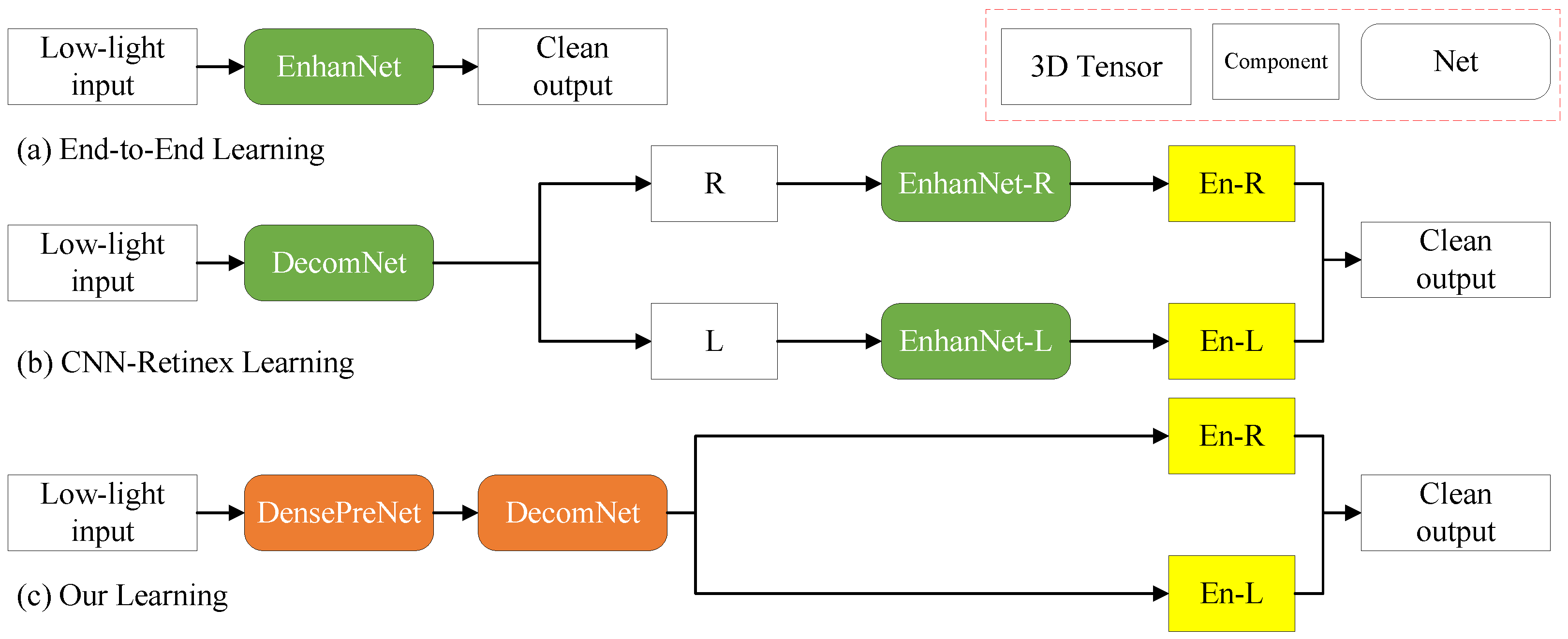
Figure 1.
Comparison of existing learning frameworks with ours for LLIE. (a) End-to-end learning framework, accepted by LLNet and MBLLEN. (b) CNN-Retinex learning framework, accepted by Retinex-Net, KinD, URetinex-Net, and PairLIE. They require enhancement networks to optimize and refine the decomposed components after the decomposition network. (c) Our approach eliminates the need for additional enhancement networks by optimizing component decoupling within the decomposition network.
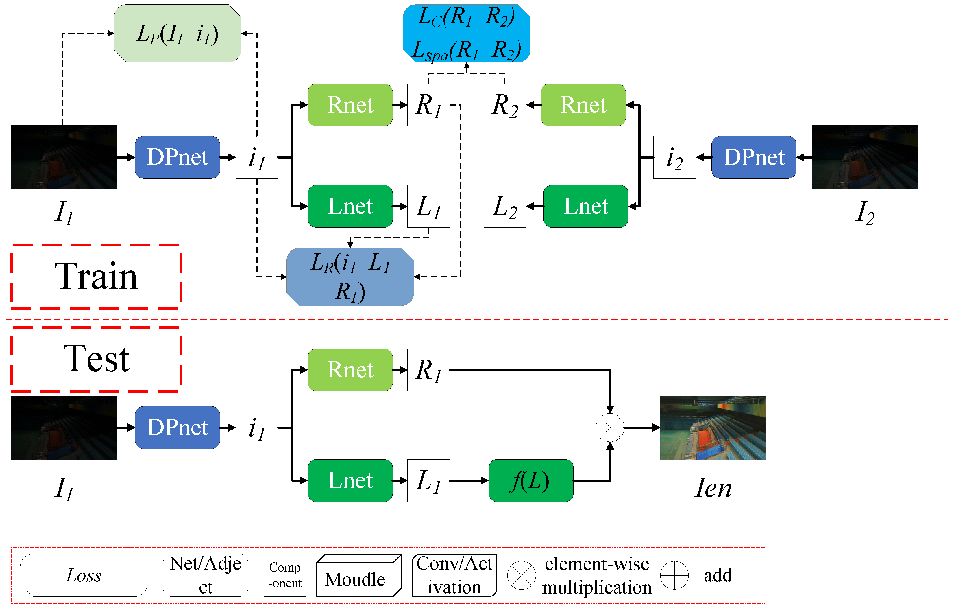
Figure 2.
The architecture of DCDNet. During training, DPnet preprocesses low-light inputs to optimize Retinex decomposition, while Rnet and Lnet represent the reflectance and illumination decomposition networks, respectively. Optimization uses four losses: (Preprocessing), (Retinex Decomposition), (Spatial Consistency), and (Reflectance Consistency). During testing, trained DPnet, Lnet, and Rnet decompose inputs into reflectance and illumination; illumination is adjusted and recombined with reflectance to output enhanced images.
Figure 3.
Overall Architecture of DPnet. DPnet aims to eliminate features incompatible with Retinex decomposition.
Figure 3.
Overall Architecture of DPnet. DPnet aims to eliminate features incompatible with Retinex decomposition.
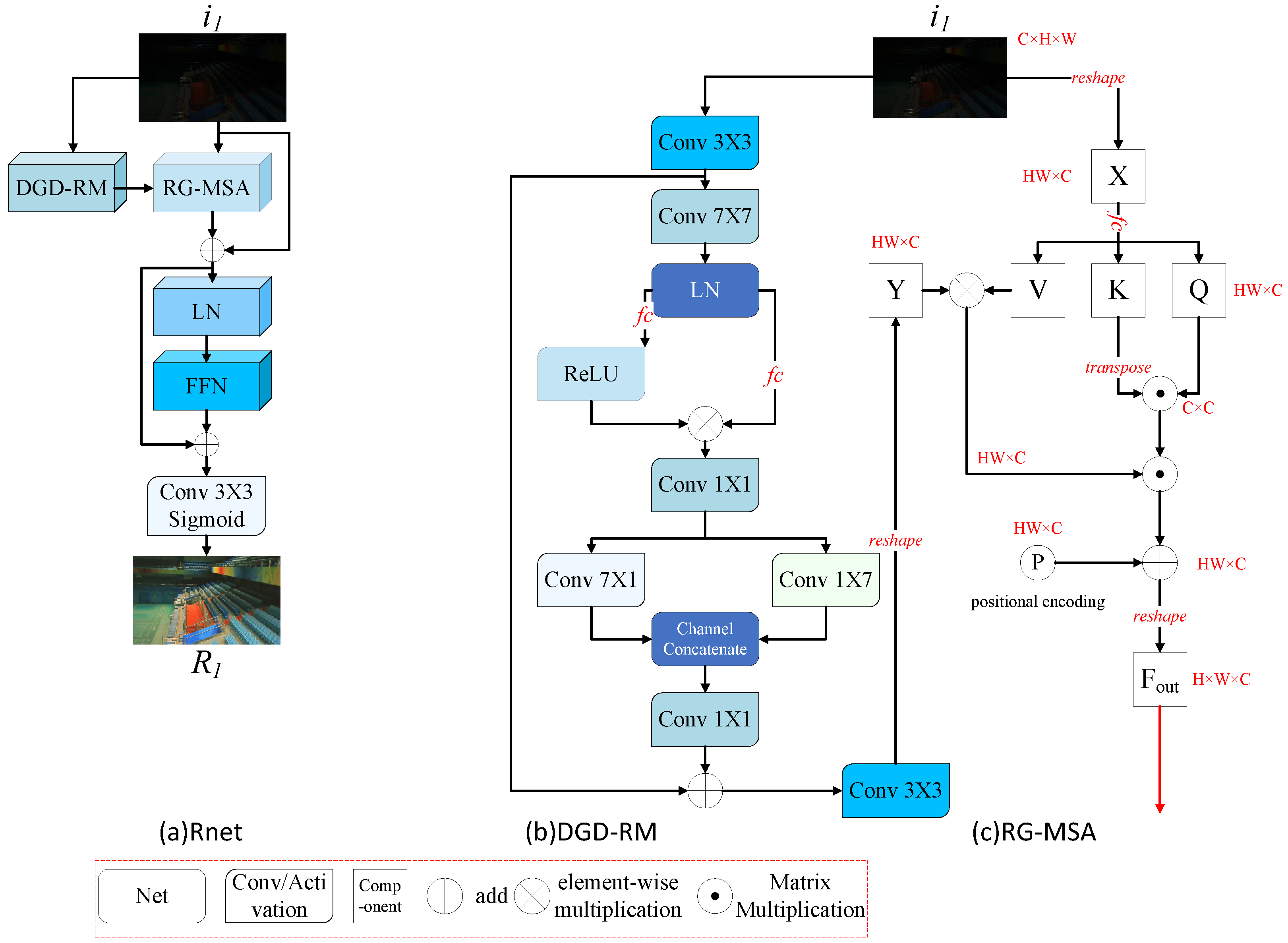
Figure 4.
(a) Shows the overall architecture of Rnet, whose key components are the DGD-RM (b) and the RG-MSA (c). Detailed structures of these two components are illustrated on the right. The RG-MSA utilizes the reflectance estimated by the DGD-RM to guide the self-attention computation. Beginning with convolution, the structure culminates in the output .
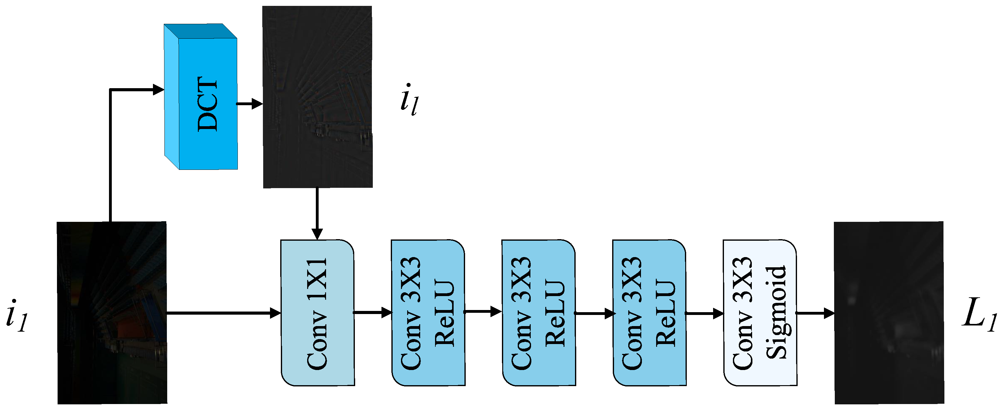
Figure 5.
Overall architecture of Lnet. Lnet incorporates a global illumination prior through DCT.
Figure 5.
Overall architecture of Lnet. Lnet incorporates a global illumination prior through DCT.
Figure 6.
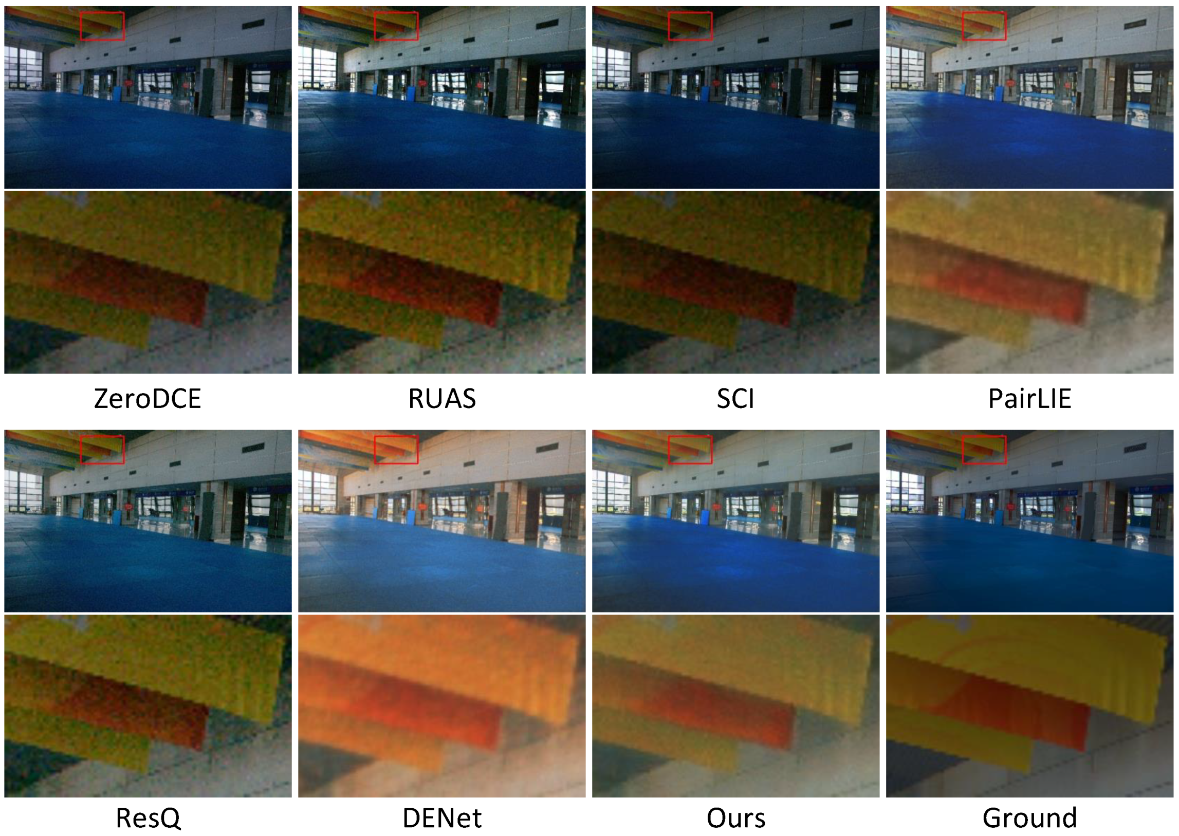
Visual comparison of the compared methods on LLIE, including ZeroDCE, RUAS, SCI, PairLIE, ResQ, DENet, and ours. The final result corresponds to the ground truth image. The dataset comes from LOL v1. The areas within the red boxes are selected for magnification, and the detailed views are presented beneath.
Figure 7.
Visual comparisons of enhancement results by using different methods: ZeroDCE, RUAS, SCI, PairLIE, ResQ, DENet, and ours. The final result corresponds to the ground truth image. The dataset comes from LOL v2. The areas within the red boxes are selected for magnification, and the detailed views are presented beneath.
Figure 8.
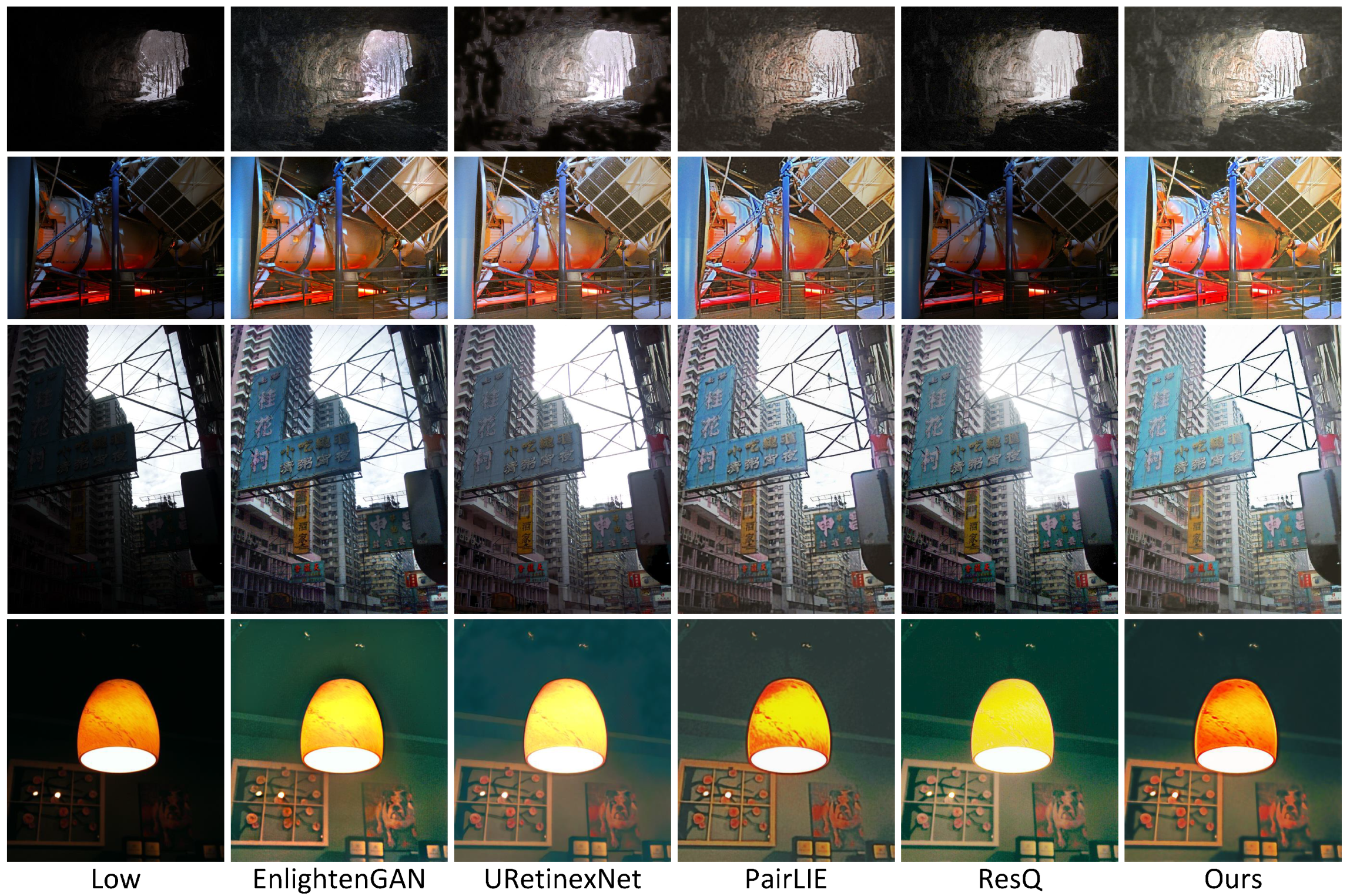
Visual comparisons of enhancement results by using different methods: EnlightenGAN, URetinexNet, PairLIE, ResQ, and ours. The datasets from top to bottom are MEF, DICM, Fusion, and LIME, respectively.
Figure 8.
Visual comparisons of enhancement results by using different methods: EnlightenGAN, URetinexNet, PairLIE, ResQ, and ours. The datasets from top to bottom are MEF, DICM, Fusion, and LIME, respectively.
Figure 9.
Visualization of the decomposed outputs. Enhanced results under different correction factors .
Figure 9.
Visualization of the decomposed outputs. Enhanced results under different correction factors .
Figure 10.
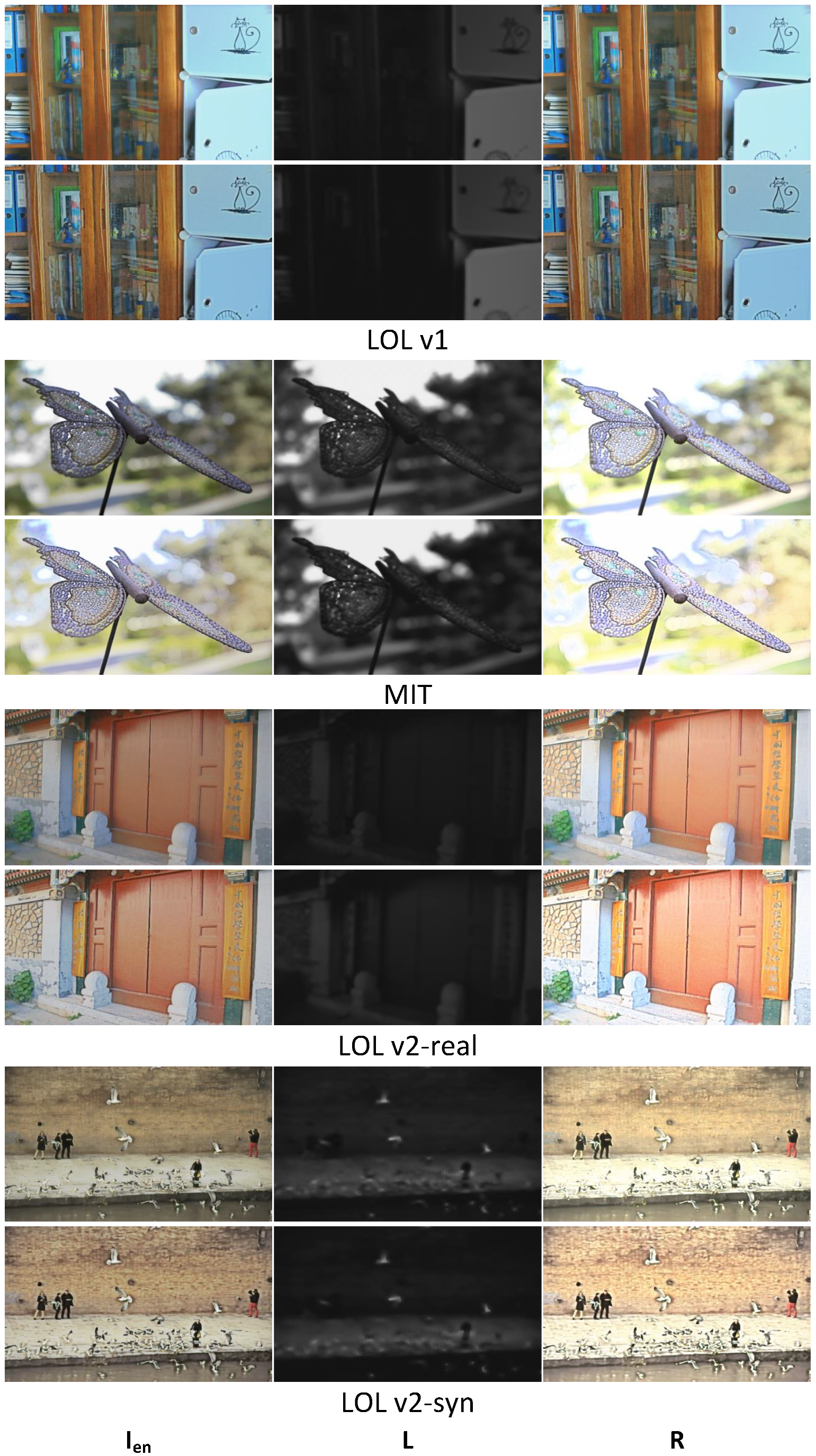
The decomposition results using our method and PairLIE. From left to right: the enhanced image (), illumination (L), and reflectance (R). The dataset comes from LOL v1, MIT and LOL v2 (LOL v2-real and LOL v2-syn).
Figure 10.
The decomposition results using our method and PairLIE. From left to right: the enhanced image (), illumination (L), and reflectance (R). The dataset comes from LOL v1, MIT and LOL v2 (LOL v2-real and LOL v2-syn).
Figure 11.
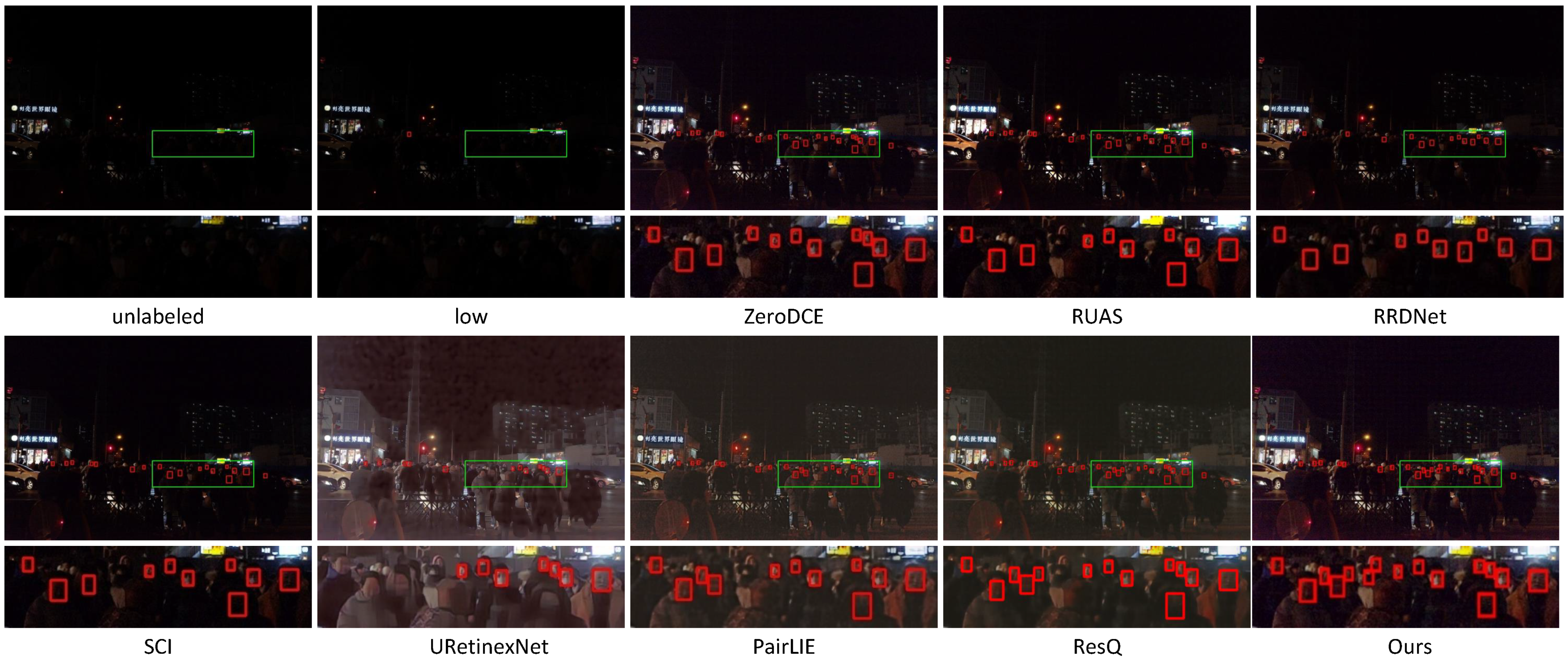
Dark face detection on a challenging example from the DARK FACE dataset, showing results from unlabeled, low, ZeroDCE, RUAS, RRDNet, SCI, URetinexNet, PairLIE, ResQ, and ours. The green boxes indicate the regions to be magnified. The enlarged views are presented below, with red boxes highlighting the detected faces.
Figure 12.
Ablation studies results on LIME dataset. (a) w/o DGD-RM & RG-MSA; (b) w/o DCT; (c) w/o ; (d) DCDNet.
Figure 12.
Ablation studies results on LIME dataset. (a) w/o DGD-RM & RG-MSA; (b) w/o DCT; (c) w/o ; (d) DCDNet.
Figure 13.
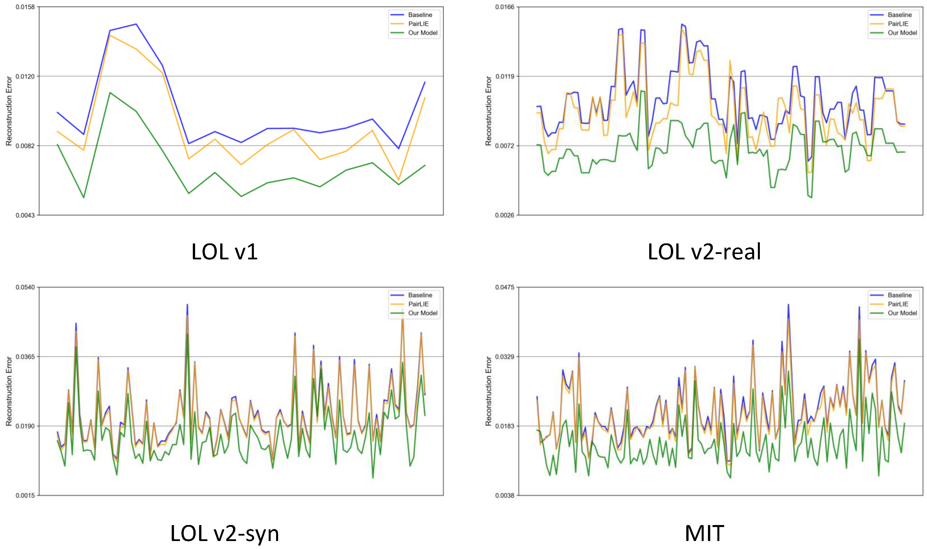
Visualization of reconstruction errors on LOL v1, LOL v2-real, LOL v2-syn, and MIT. Baseline decomposes original low-light images (blue); PairLIE uses its Pnet on projected images (orange); our method employs DPnet on projected images (green).
Figure 13.
Visualization of reconstruction errors on LOL v1, LOL v2-real, LOL v2-syn, and MIT. Baseline decomposes original low-light images (blue); PairLIE uses its Pnet on projected images (orange); our method employs DPnet on projected images (green).
Figure 14.
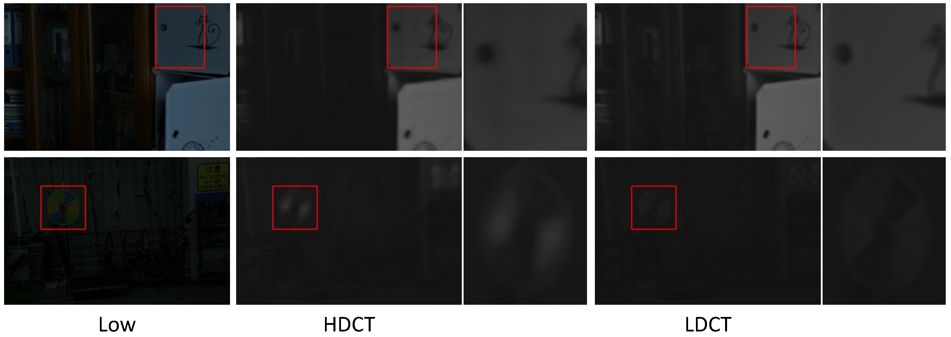
Illuminationmaps from HDCT vs. LDCT. LDCT is better. From left to right: low, HDCT, and LDCT. The red boxes indicate the regions to be magnified; the zoomed-in views are presented on the right.
Figure 14.
Illuminationmaps from HDCT vs. LDCT. LDCT is better. From left to right: low, HDCT, and LDCT. The red boxes indicate the regions to be magnified; the zoomed-in views are presented on the right.
Figure 15.
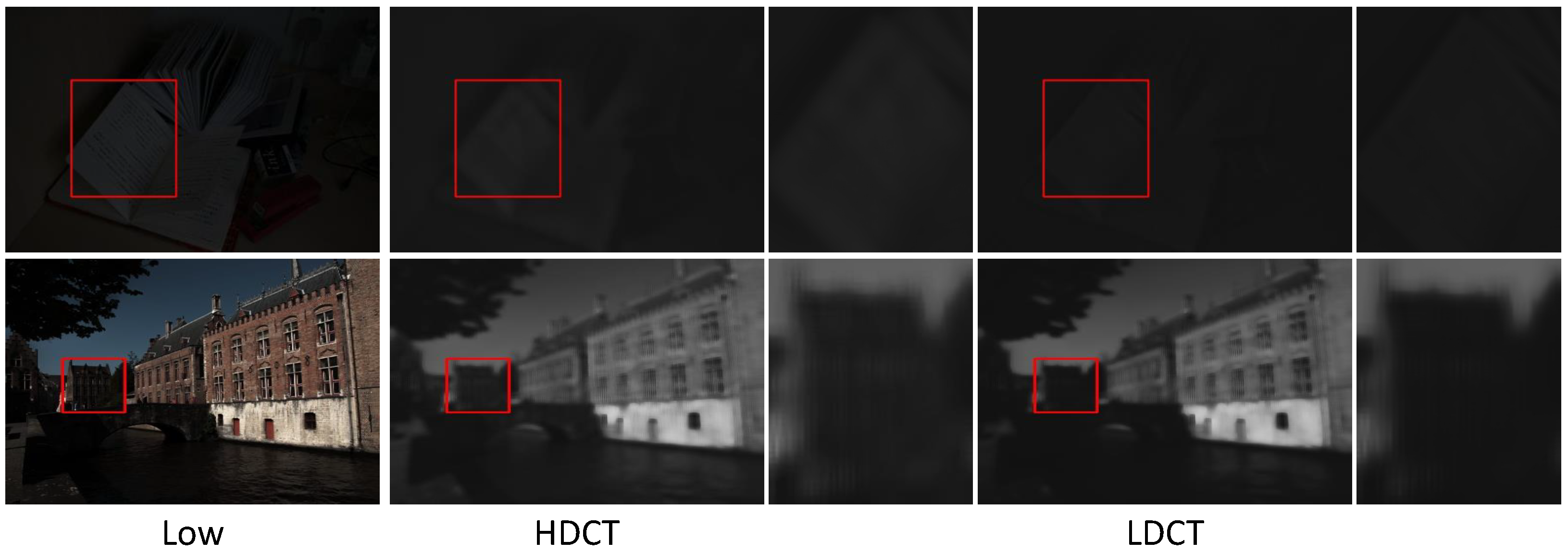
Illuminationmaps from HDCT vs. LDCT. HDCT is better. From left to right: low, HDCT, and LDCT. The red boxes indicate the regions to be magnified; the zoomed-in views are presented on the right.
Figure 15.
Illuminationmaps from HDCT vs. LDCT. HDCT is better. From left to right: low, HDCT, and LDCT. The red boxes indicate the regions to be magnified; the zoomed-in views are presented on the right.
Figure 16.
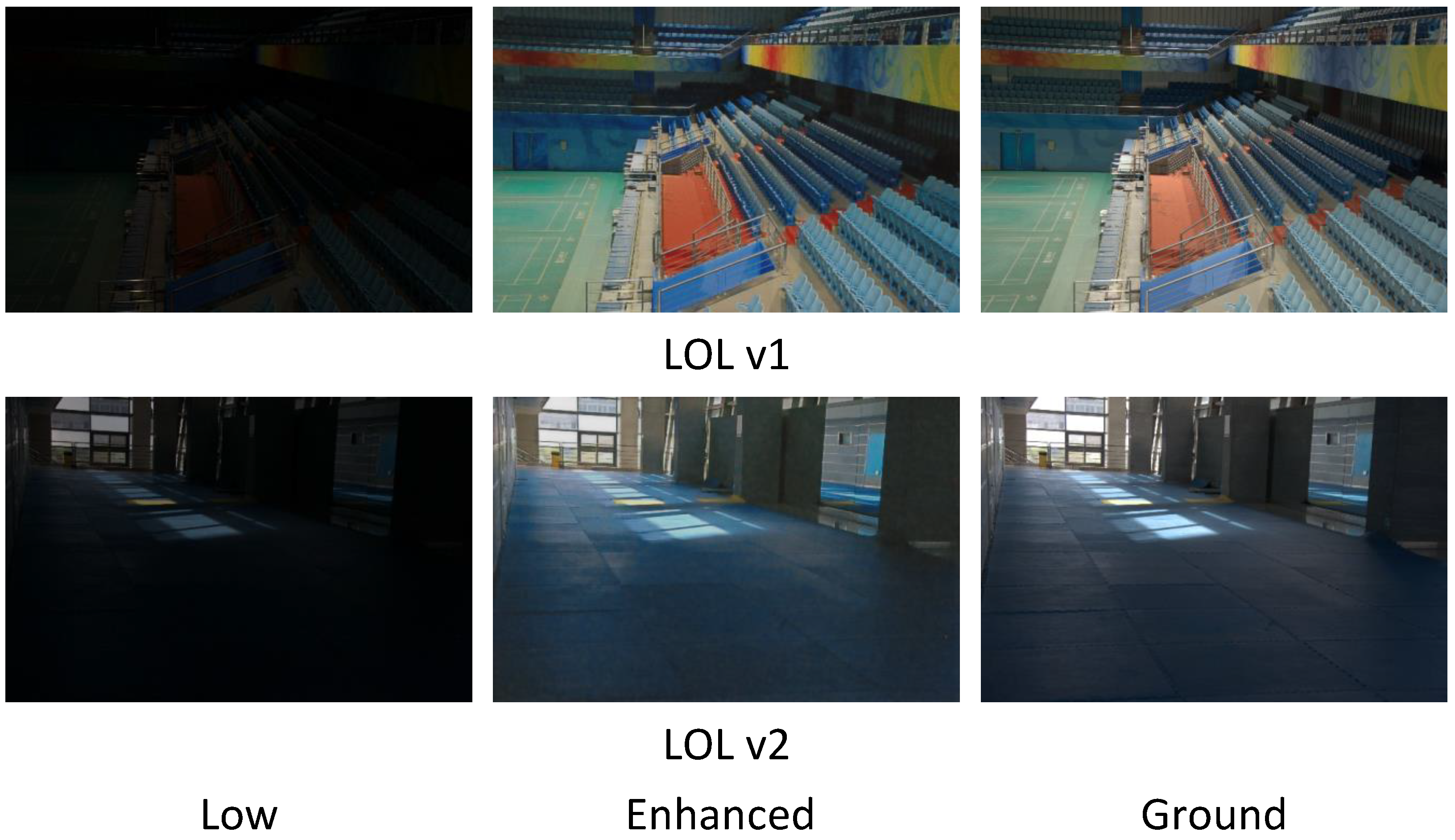
Comparison chart of failure case results. Among them, from left to right, are the low-light image, the enhanced image, and the label image in that order. The datasets come from LOL v1 and LOL v2.
Figure 16.
Comparison chart of failure case results. Among them, from left to right, are the low-light image, the enhanced image, and the label image in that order. The datasets come from LOL v1 and LOL v2.
Table 1.
Network architecture specifications. The 32 indicates the use of the DGD-RM and RG-MSA modules here. The 6 indicates the use of the DCT module here.
Table 1.
Network architecture specifications. The 32 indicates the use of the DGD-RM and RG-MSA modules here. The 6 indicates the use of the DCT module here.
| Network | Dimensional Changes | Layer Depth | Convolution Kernel |
|---|
| DPnet | 3 (input) — 16 — 16 — 16 — 3 (output) | 4 | |
| Rnet | 3 (input) — 32 — 3 — 32 — 3 (output) | 4 | |
| Lnet | 3 (input) — 6 — 32 — 32 — 32 — 1 (output) | 5 | & |
Table 2.
Conduct a quantitative evaluation of comparative methods on three reference benchmark datasets. The best and second-best results are marked in red and blue, respectively. ↑ (or ↓) means that the larger (or smaller), the better. “Supervised” denotes supervised methods and “Unsupervised” denotes unsupervised methods.
| Method | LOL v1 | LOL v2-Real | LOL v2-Synthetic | MIT |
|---|
| PSNR ↑ | SSIM ↑ | LPIPS ↓ | PSNR ↑ | SSIM ↑ | LPIPS ↓ | PSNR ↑ | SSIM ↑ | LPIPS ↓ | PSNR ↑ | SSIM ↑ | LPIPS ↓ |
|---|
| Supervised | | | | | | | | | | | | |
| Retinex-Net [6] | 14.98 | 0.327 | 0.624 | 16.10 | 0.401 | 0.543 | 14.04 | 0.273 | 0.818 | 14.73 | 0.738 | 0.382 |
| MBLLEN [5] | 17.86 | 0.627 | 0.225 | 17.87 | 0.694 | 0.272 | 15.78 | 0.501 | 0.599 | 18.01 | 0.751 | 0.283 |
| KinD [7] | 16.15 | 0.620 | 0.421 | 19.00 | 0.737 | 0.279 | 16.31 | 0.568 | 0.552 | 17.84 | 0.768 | 0.250 |
| URetinex-Net [9] | 17.28 | 0.697 | 0.311 | 21.09 | 0.757 | 0.100 | 17.70 | 0.629 | 0.448 | 18.56 | 0.822 | 0.188 |
| SNR-Aware [12] | 24.61 | 0.842 | 0.233 | 21.48 | 0.849 | 0.237 | 24.14 | 0.928 | 0.189 | - | - | - |
| Retinexformer [13] | 23.93 | 0.831 | 0.125 | 22.45 | 0.844 | 0.165 | 25.67 | 0.930 | 0.059 | - | - | - |
| CIDNet [40] | 23.81 | 0.870 | 0.086 | 24.11 | 0.867 | 0.116 | 25.12 | 0.939 | 0.045 | - | - | - |
| DiffLight [41] | 25.85 | 0.876 | 0.082 | - | - | - | - | - | - | - | - | |
| CWNet [42] | 23.60 | 0.849 | 0.065 | 27.39 | 0.900 | 0.038 | 25.50 | 0.936 | 0.020 | - | - | - |
| Unsupervised | | | | | | | | | | | | |
| EnlightGAN [20] | 17.56 | 0.665 | 0.316 | 18.68 | 0.673 | 0.301 | 15.18 | 0.482 | 0.620 | 15.56 | 0.800 | 0.213 |
| RRDNet [11] | 10.16 | 0.406 | 0.483 | 13.70 | 0.508 | 0.290 | 10.50 | 0.310 | 0.729 | 19.60 | 0.830 | 0.229 |
| UEGAN [43] | 8.24 | 0.222 | 0.689 | 12.81 | 0.268 | 0.410 | 8.90 | 0.193 | 0.700 | 19.54 | 0.870 | 0.199 |
| ZeroDCE [22] | 15.33 | 0.567 | 0.335 | 18.46 | 0.580 | 0.305 | 12.99 | 0.365 | 0.684 | 17.96 | 0.843 | 0.226 |
| RUAS [28] | 16.15 | 0.462 | 0.368 | 14.89 | 0.455 | 0.372 | 12.19 | 0.297 | 0.748 | 8.46 | 0.540 | 0.585 |
| SCI [44] | 14.78 | 0.522 | 0.340 | 17.30 | 0.534 | 0.308 | 12.36 | 0.323 | 0.701 | 19.52 | 0.885 | 0.176 |
| PairLIE [14] | 19.51 | 0.736 | 0.248 | 18.23 | 0.735 | 0.260 | 16.11 | 0.566 | 0.560 | 14.47 | 0.759 | 0.198 |
| ResQ [45] | 18.28 | 0.596 | 0.323 | 19.67 | 0.573 | 0.347 | 15.65 | 0.394 | 0.687 | 20.87 | 0.915 | 0.107 |
| DENet [26] | 19.80 | 0.750 | 0.253 | 20.22 | 0.793 | 0.266 | 18.24 | 0.796 | 0.268 | 20.30 | 0.876 | 0.193 |
| Ours | 20.87 | 0.770 | 0.197 | 20.35 | 0.810 | 0.191 | 19.70 | 0.810 | 0.200 | 21.66 | 0.864 | 0.164 |
Table 3.
Conduct quantitative evaluation of comparative methods using NIQE on five no-reference benchmark datasets. The best and second-best results are marked in red and blue, respectively.
Table 3.
Conduct quantitative evaluation of comparative methods using NIQE on five no-reference benchmark datasets. The best and second-best results are marked in red and blue, respectively.
| Method | No-Reference Benchmark Dataset | Average |
|---|
| MEF | DICM | LIME | Fusion | VV |
|---|
| EnlightenGAN [20] | 3.420 | 3.568 | 4.061 | 3.654 | 2.823 | 3.505 |
| RRDNet [11] | 3.781 | 6.727 | 6.125 | 5.781 | 2.979 | 5.078 |
| UEGAN [43] | 5.132 | 4.046 | 4.540 | 4.228 | 3.696 | 4.328 |
| RUAS [28] | 5.109 | 5.727 | 4.697 | 6.080 | 5.346 | 5.392 |
| URetinexNet [9] | 3.789 | 3.459 | 4.341 | 3.818 | 3.019 | 3.685 |
| SNR-Aware [12] | 4.180 | 4.712 | 5.742 | 4.323 | 9.872 | 5.765 |
| PairLIE [14] | 4.164 | 3.519 | 4.515 | 5.002 | 3.654 | 4.171 |
| Retinexformer [13] | 4.322 | 3.853 | 4.310 | 3.762 | 3.094 | 3.869 |
| ResQ [45] | 3.477 | 3.388 | 4.034 | 3.632 | 2.732 | 3.453 |
| CWNet [42] | 3.568 | 3.795 | 4.138 | 4.025 | 3.214 | 3.747 |
| Ours | 3.462 | 3.027 | 4.000 | 3.662 | 2.951 | 3.420 |
Table 4.
Quantitative evaluation of deep-learning-based methods on model complexity in terms of Flops, Params, and inference time (Gpu seconds). “Supervised” denotes supervised methods and “Unsupervised” denotes unsupervised methods.
Table 4.
Quantitative evaluation of deep-learning-based methods on model complexity in terms of Flops, Params, and inference time (Gpu seconds). “Supervised” denotes supervised methods and “Unsupervised” denotes unsupervised methods.
| Method | FLOPs (G) | Params (M) | Time (S) |
|---|
| Supervised | | | |
| Retinex-Net [6] | 136.02 | 0.8383 | 0.0864 |
| MBLLEN [5] | 60.02 | 0.4502 | 0.2111 |
| KinD [7] | 29.13 | 8.5402 | 0.1529 |
| URetinex-Net [9] | 58.27 | 0.3621 | 0.0176 |
| SNR-Aware [12] | 27.88 | 4.0132 | 0.0266 |
| Retinexformer [13] | 17.02 | 1.6057 | 0.0234 |
| CIDNet [40] | 7.57 | 1.88 | - |
| DifLight [41] | 168.3 | - | - |
| CWNet [42] | 11.3 | 1.23 | - |
| Unsupervised | | | |
| EnlightenGAN [20] | 61.01 | 8.6360 | 0.0701 |
| RRDNet [11] | 30.66 | 0.1282 | 1.5677 |
| UEGAN [43] | 32.72 | 16.6149 | 0.0435 |
| ZeroDCE [22] | 5.21 | 0.0789 | 0.0204 |
| RUAS [28] | 0.21 | 0.0034 | 0.0165 |
| SCI [44] | 0.08 | 0.0004 | 0.0160 |
| PairLIE [14] | 22.35 | 0.3418 | 0.1985 |
| ResQ [45] | 0.49 | 0.0123 | 0.0178 |
| DENet [26] | 20.40 | 0.312 | 0.0517 |
| Ours | 7.00 | 0.107 | 0.0085 |
Table 5.
Ablation studies results on LOL v1, LOL v2-real, LOL v2-syn, and MIT datasets. The best results is marked in red, respectively. ↑ (or ↓) means that the larger (or smaller), the better.
Table 5.
Ablation studies results on LOL v1, LOL v2-real, LOL v2-syn, and MIT datasets. The best results is marked in red, respectively. ↑ (or ↓) means that the larger (or smaller), the better.
| Setting | LOL v1 | LOL v2-Real | LOL v2-Syn | MIT |
|---|
| PSNR ↑ | SSIM ↑ | LPIPS ↓ | PSNR ↑ | SSIM ↑ | LPIPS ↓ | PSNR ↑ | SSIM ↑ | LPIPS ↓ | PSNR ↑ | SSIM ↑ | LPIPS ↓ |
|---|
| (a) w/o DGD-RM & RG-MSA | 19.72 | 0.707 | 0.243 | 19.90 | 0.769 | 0.238 | 19.03 | 0.732 | 0.230 | 20.81 | 0.836 | 0.192 |
| (b) w/o DCT | 20.36 | 0.736 | 0.232 | 19.54 | 0.755 | 0.221 | 19.30 | 0.752 | 0.235 | 21.20 | 0.847 | 0.179 |
| (c) w/o | 20.45 | 0.747 | 0.221 | 20.13 | 0.798 | 0.201 | 19.47 | 0.795 | 0.202 | 21.45 | 0.850 | 0.178 |
| DCDNet | 20.87 | 0.770 | 0.197 | 20.35 | 0.810 | 0.191 | 19.70 | 0.810 | 0.200 | 21.66 | 0.864 | 0.164 |
Table 6.
Conduct quantitative evaluation of comparative baseline, Pnet and DPnet (ours), on four reference benchmark datasets. The better results are marked in red, respectively. ↓ means that the smaller the better.
Table 6.
Conduct quantitative evaluation of comparative baseline, Pnet and DPnet (ours), on four reference benchmark datasets. The better results are marked in red, respectively. ↓ means that the smaller the better.
| Method | LOL v1 | LOL v2-Real | LOL v2-Synthetic | MIT |
|---|
| Reconstruction Error ↓ | Reconstruction Error ↓ | Reconstruction Error ↓ | Reconstruction Error ↓ |
|---|
| Baseline | 0.0101 | 0.0104 | 0.0221 | 0.0217 |
| Pnet | 0.0092 | 0.0096 | 0.0216 | 0.0211 |
| DPnet (Ours) | 0.0070 | 0.0071 | 0.0168 | 0.0149 |
Table 7.
Conduct quantitative evaluation of comparative HDCT and LDCT on three reference benchmark datasets. The better results are marked in red, respectively. ↑ (or ↓) means that the larger (or smaller), the better.
Table 7.
Conduct quantitative evaluation of comparative HDCT and LDCT on three reference benchmark datasets. The better results are marked in red, respectively. ↑ (or ↓) means that the larger (or smaller), the better.
| Method | LOL v1 | LOL v2-Real | LOL v2-Synthetic | MIT |
|---|
| PSNR ↑ | SSIM ↑ | LPIPS ↓ | PSNR ↑ | SSIM ↑ | LPIPS ↓ | PSNR ↑ | SSIM ↑ | LPIPS ↓ | PSNR ↑ | SSIM ↑ | LPIPS ↓ |
|---|
| HDCT | 20.65 | 0.750 | 0.217 | 20.16 | 0.785 | 0.210 | 19.23 | 0.804 | 0.202 | 21.33 | 0.859 | 0.160 |
| LDCT (our) | 20.87 | 0.770 | 0.197 | 20.35 | 0.810 | 0.191 | 19.70 | 0.810 | 0.200 | 21.66 | 0.864 | 0.164 |
