
Enhancing Manufacturing Precision: Leveraging Motor Currents Data of Computer Numerical Control Machines for Geometrical Accuracy Prediction Through Machine Learning


Abstract
1. Introduction
2. Materials and Methods
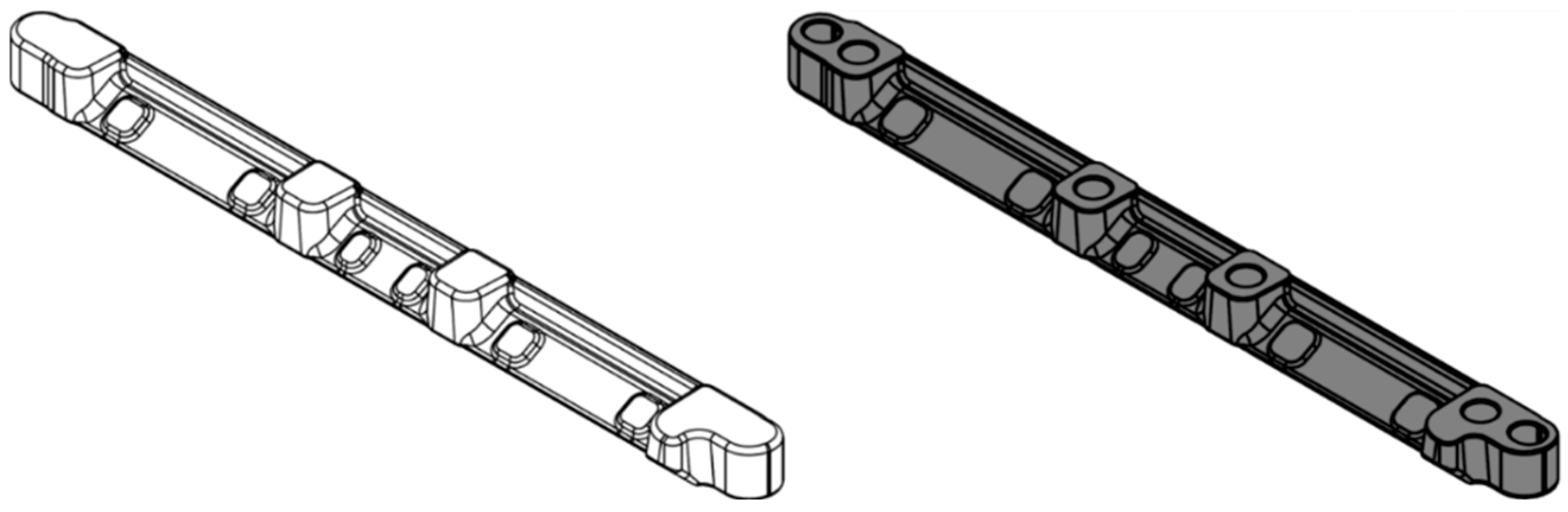
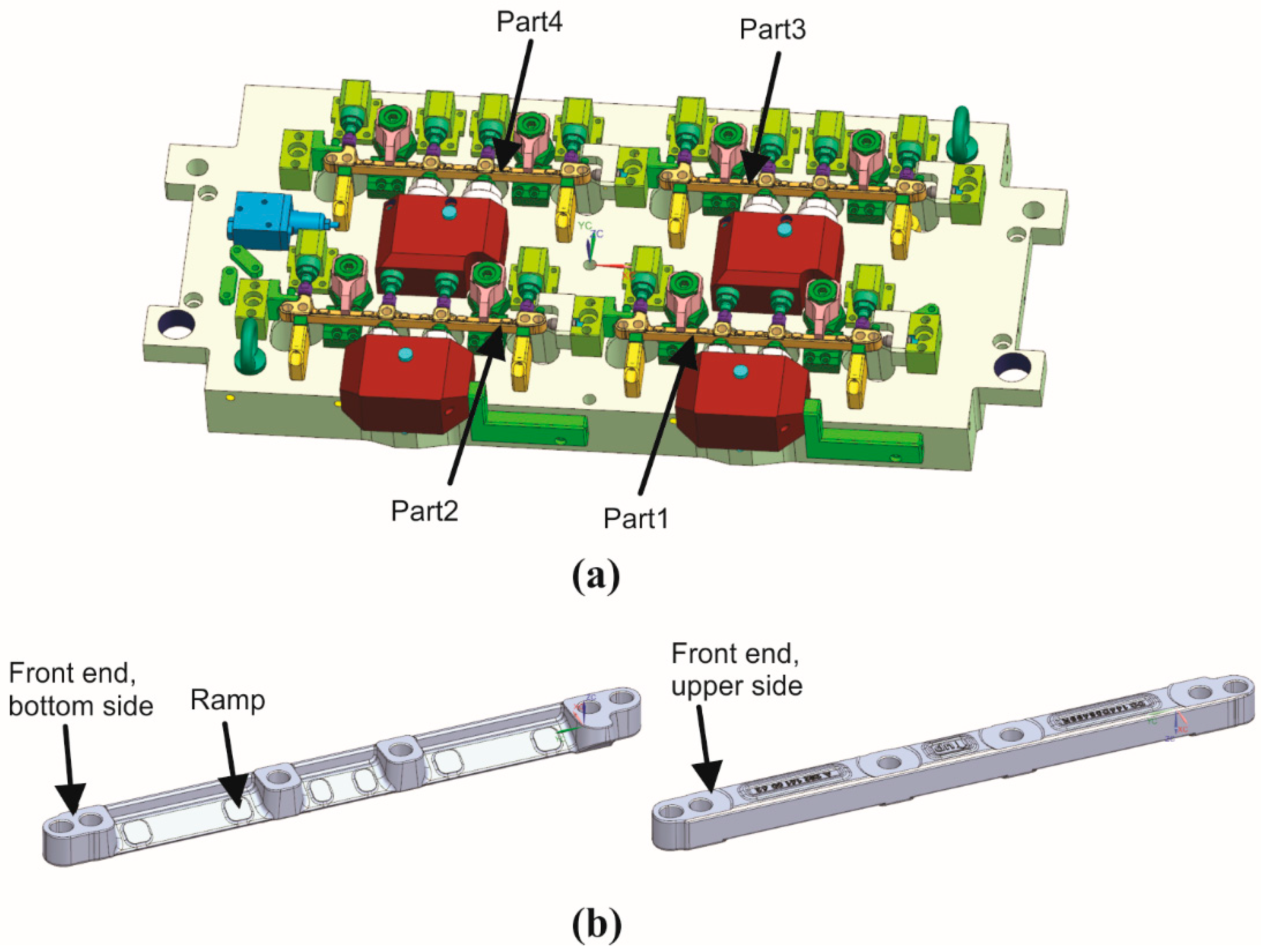
2.1. Processed Part and Overall Structure of the Proposed Procedure
- –
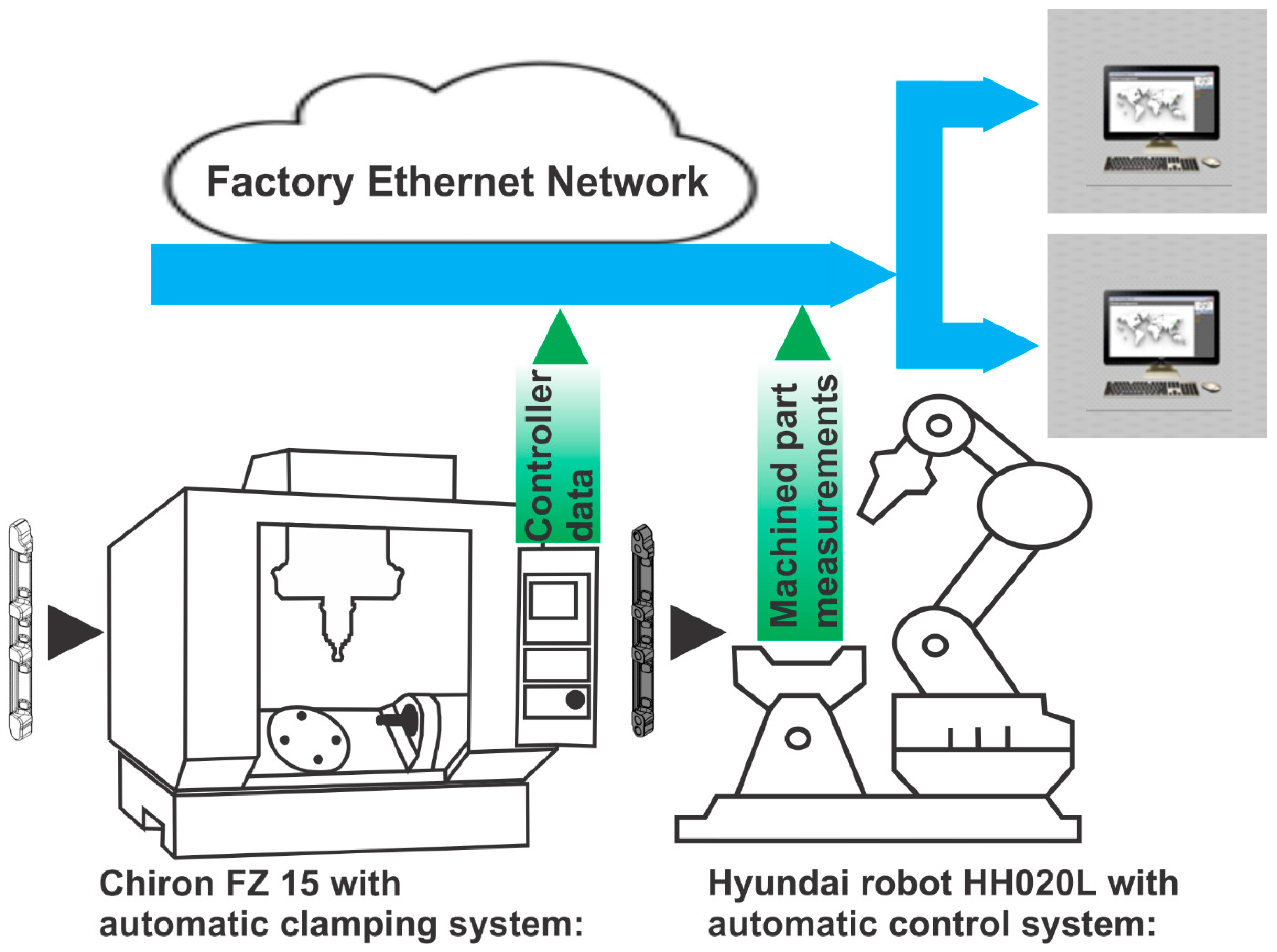
- Two-spindle 4-axis milling machines, Chiron DZ15W, with pallet changer. Milling machines are general-purpose without any adaptations for the manufacturing cell. The machines are equipped with Fanuc 3li-model B5 controllers.
- –
- An automatic clamping system. Clamping is performed by an automated hydraulic clamping device.
- –
- Hyundai robot HH010L, which serves the manufacturing cell. This 6-axis industrial robot executes clamping/unclamping parts in the milling machine and placing them in/from the control station.
- –
- An automatic control station for 100% control of the machined parts. This uses measurement probes from the Keyence company.
2.2. Machining Process and Control Measurement Device
2.3. Controller Data, Part Accuracy Measurements, and Data Preprocessing
2.4. Feature Extraction
2.5. Machine Learning Algorithms
- –
- Random Forest,
- –
- K-nearest neighbors, and
- –
- Decision Trees.
3. Results
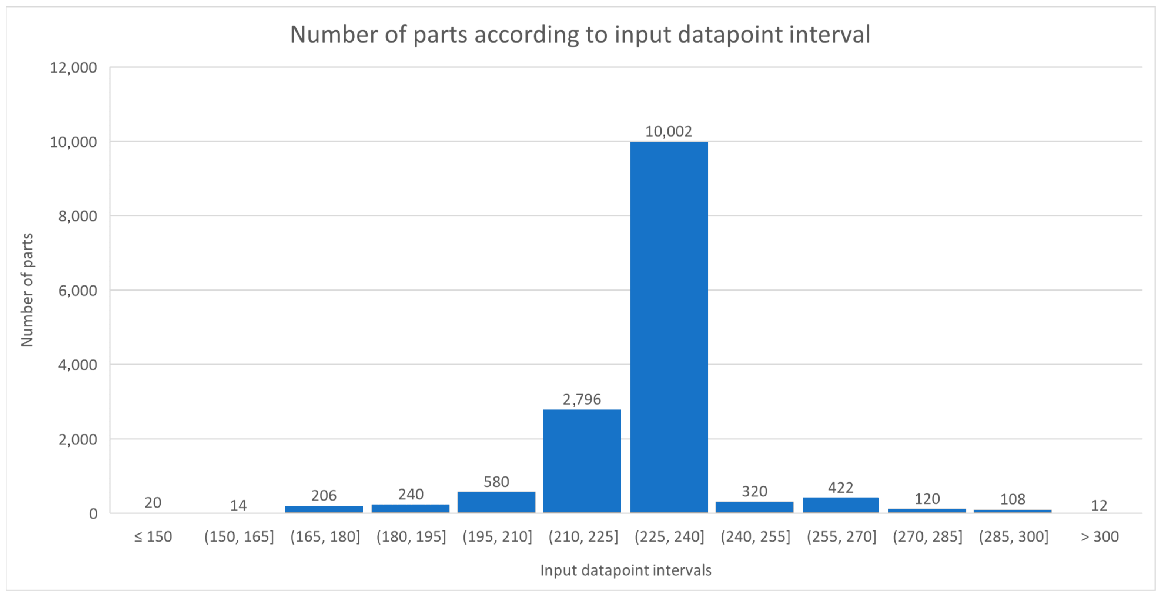
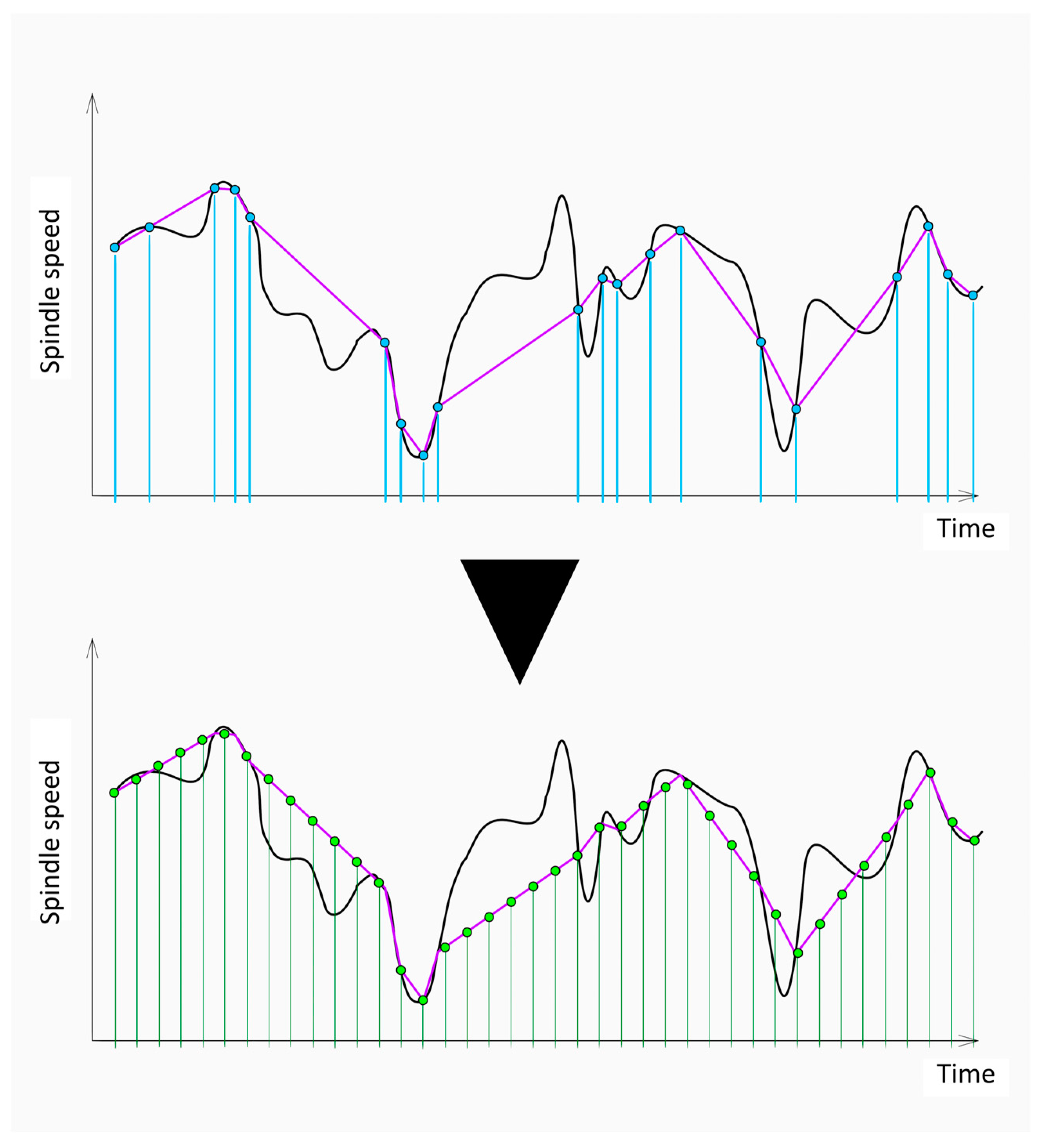
3.1. Analysis of Gathered Controller Data and Time-Series Preprocessing
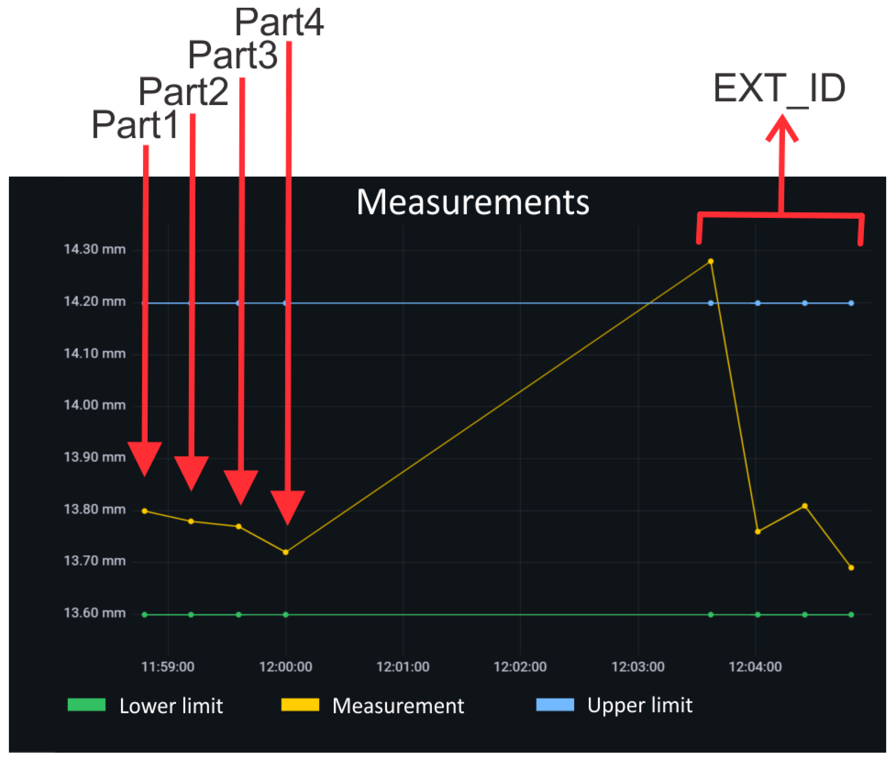
3.2. Pairing of Controller Data and Part Accuracy Measurements
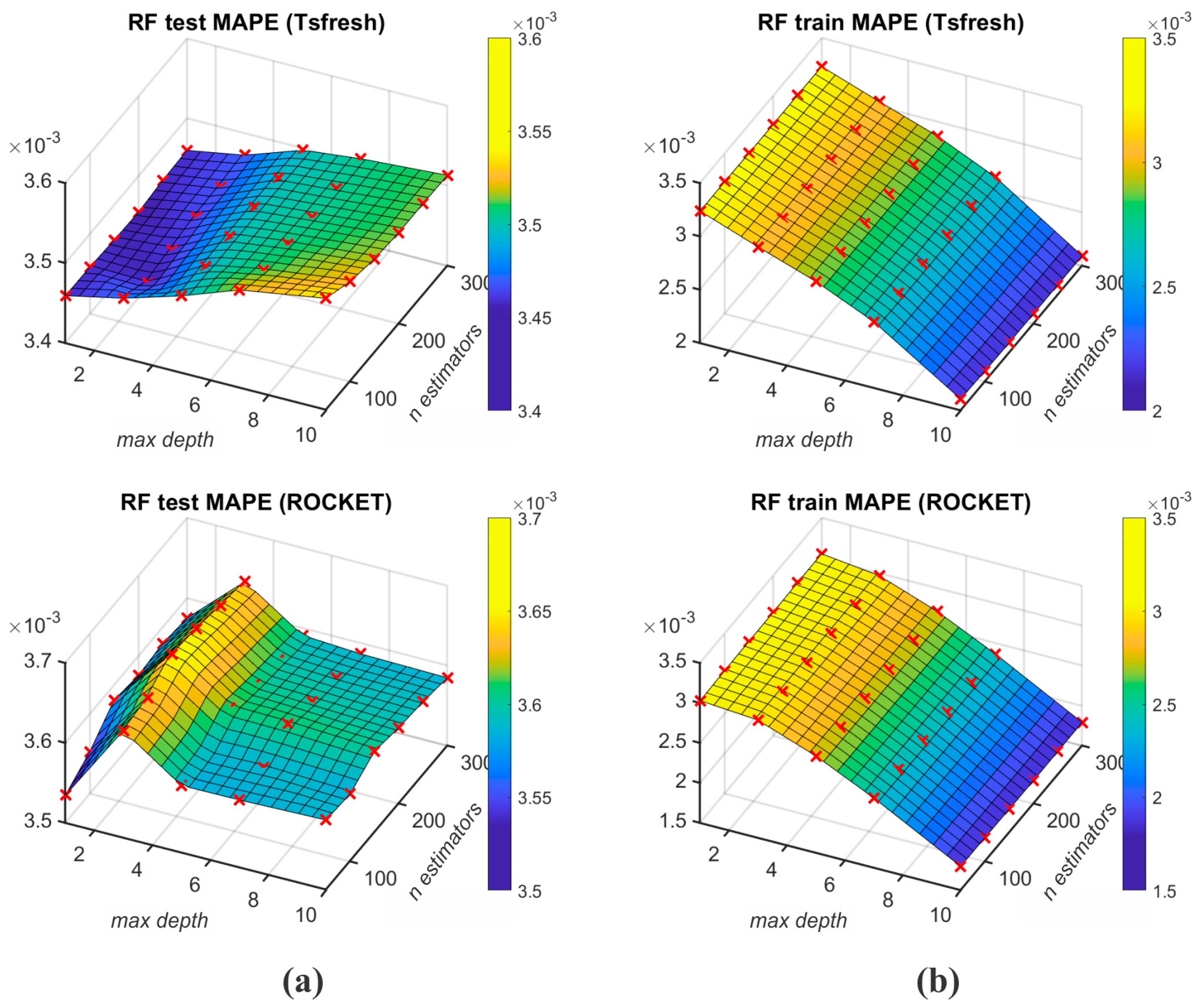
3.3. Machine Learning
4. Discussion
Author Contributions
Funding
Informed Consent Statement
Data Availability Statement
Conflicts of Interest
References
- Tao, F.; Qi, Q. New IT Driven Service-Oriented Smart Manufacturing: Framework and Characteristics. IEEE Trans. Syst. Man Cybern. Syst. 2019, 49, 81–91. [Google Scholar] [CrossRef]
- O’Donovan, P.; Leahy, K.; Bruton, K.; O’Sullivan, D. An industrial big data pipeline for data-driven analytics maintenance applications in large-scale smart manufacturing facilities. J. Big Data 2015, 2, 25. [Google Scholar] [CrossRef]
- Yin, S.; Kaynak, O. Big Data for Modern Industry: Challenges and Trends [Point of View]. Proc. IEEE 2015, 103, 143–146. [Google Scholar] [CrossRef]
- Tao, F.; Qi, Q.; Liu, A.; Kusiak, A. Data-driven smart manufacturing. J. Manuf. Syst. 2018, 48, 157–169. [Google Scholar] [CrossRef]
- Yang, C.; Shen, W.; Wang, X. Applications of Internet of Things in manufacturing. In Proceedings of the 2016 IEEE 20th International Conference on Computer Supported Cooperative Work in Design (CSCWD), Nanchang, China, 4–6 May 2016; pp. 670–675. [Google Scholar] [CrossRef]
- Yang, C.; Shen, W.; Wang, X. The Internet of Things in Manufacturing: Key Issues and Potential Applications. IEEE Syst. Man Cybern. Mag. 2018, 4, 6–15. [Google Scholar] [CrossRef]
- Zhong, R.Y.; Ge, W. Internet of things enabled manufacturing: A review. Int. J. Agil. Syst. Manag. 2018, 11, 126–154. [Google Scholar] [CrossRef]
- Siderska, J.; Jadaan, K.S. Cloud manufacturing: A service-oriented manufacturing paradigm. A review paper. Eng. Manag. Prod. Serv. 2018, 10, 22–31. [Google Scholar] [CrossRef]
- Lee, J.; Davari, H.; Singh, J.; Pandhare, V. Industrial Artificial Intelligence for industry 4.0-based manufacturing systems. Manuf. Lett. 2018, 18, 20–23. [Google Scholar] [CrossRef]
- Li, B.-H.; Hou, B.-C.; Yu, W.-T.; Lu, X.-B.; Yang, C.-W. Applications of artificial intelligence in intelligent manufacturing: A review. Front. Inf. Technol. Electron. Eng. 2017, 18, 86–96. [Google Scholar] [CrossRef]
- Kumar, S.L. State of The Art-Intense Review on Artificial Intelligence Systems Application in Process Planning and Manufacturing. Eng. Appl. Artif. Intell. 2017, 65, 294–329. [Google Scholar] [CrossRef]
- Cioffi, R.; Travaglioni, M.; Piscitelli, G.; Petrillo, A.; De Felice, F. Artificial Intelligence and Machine Learning Applications in Smart Production: Progress, Trends, and Directions. Sustainability 2020, 12, 492. [Google Scholar] [CrossRef]
- Korkmaz, M.; Yaşar, N. FEM modelling of turning of AA6061-T6: Investigation of chip morphology, chip thickness and shear angle. J. Prod. Syst. Manuf. Sci. 2021, 2, 50–58. [Google Scholar]
- Nasir, V.; Sassani, F. A review on deep learning in machining and tool monitoring: Methods, opportunities, and challenges. Int. J. Adv. Manuf. Technol. 2021, 115, 2683–2709. [Google Scholar] [CrossRef]
- Wang, B.; Liu, Z. Influences of tool structure, tool material and tool wear on machined surface integrity during turning and milling of titanium and nickel alloys: A review. Int. J. Adv. Manuf. Technol. 2018, 98, 1925–1975. [Google Scholar] [CrossRef]
- Yeganefar, A.; Niknam, S.A.; Asadi, R. The use of support vector machine, neural network, and regression analysis to predict and optimize surface roughness and cutting forces in milling. Int. J. Adv. Manuf. Technol. 2019, 105, 951–965. [Google Scholar] [CrossRef]
- Nasir, V.; Cool, J. Intelligent wood machining monitoring using vibration signals combined with self-organizing maps for automatic feature selection. Int. J. Adv. Manuf. Technol. 2020, 108, 1811–1825. [Google Scholar] [CrossRef]
- Nasir, V.; Cool, J. Optimal power consumption and surface quality in the circular sawing process of Douglas-fir wood. Eur. J. Wood Wood Prod. 2019, 77, 609–617. [Google Scholar] [CrossRef]
- Nasir, V.; Mohammadpanah, A.; Cool, J. The effect of rotation speed on the power consumption and cutting accuracy of guided circular saw: Experimental measurement and analysis of saw critical and flutter speeds. Wood Mater. Sci. Eng. 2018, 15, 140–146. [Google Scholar] [CrossRef]
- Serin, G.; Sener, B.; Ozbayoglu, A.M.; Unver, H.O. Review of tool condition monitoring in machining and opportunities for deep learning. Int. J. Adv. Manuf. Technol. 2020, 109, 953–974. [Google Scholar] [CrossRef]
- Wang, M.; Wang, J. CHMM for tool condition monitoring and remaining useful life prediction. Int. J. Adv. Manuf. Technol. 2012, 59, 463–471. [Google Scholar] [CrossRef]
- Chen, W.; Liu, H.; Sun, Y.; Yang, K.; Zhang, J. A novel simulation method for interaction of machining process and machine tool structure. Int. J. Adv. Manuf. Technol. 2017, 88, 3467–3474. [Google Scholar] [CrossRef]
- Quintana, G.; Ciurana, J. Chatter in machining processes: A review. Int. J. Mach. Tools. Manuf. 2011, 51, 363–376. [Google Scholar] [CrossRef]
- Licow, R.; Chuchala, D.; Deja, M.; Orlowski, K.A.; Taube, P. Effect of pine impregnation and feed speed on sound level and cutting power in wood sawing. J. Clean. Prod. 2020, 272, 122833. [Google Scholar] [CrossRef]
- Said, Z.; Gupta, M.; Hegab, H.; Arora, N.; Khan, A.M.; Jamil, M.; Bellos, E. A comprehensive review on minimum quantity lubrication (MQL) in machining processes using nano-cutting fluids. Int. J. Adv. Manuf. Technol. 2019, 105, 2057–2086. [Google Scholar] [CrossRef]
- Mia, M.; Gupta, M.K.; Singh, G.; Królczyk, G.; Pimenov, D.Y. An approach to cleaner production for machining hardened steel using different cooling-lubrication conditions. J. Clean. Prod. 2018, 187, 1069–1081. [Google Scholar] [CrossRef]
- Bello, O.; Holzmann, J.; Yaqoob, T.; Teodoriu, C. Application Of Artificial Intelligence Methods In Drilling System Design And Operations: A Review Of The State Of The Art. J. Artif. Intell. Soft Comput. Res. 2015, 5, 121–139. [Google Scholar] [CrossRef]
- Ranjan, J.; Patra, K.; Szalay, T.; Mia, M.; Gupta, M.K.; Song, Q.; Krolczyk, G.; Chudy, R.; Pashnyov, V.A.; Pimenov, D.Y. Artificial Intelligence-Based Hole Quality Prediction in Micro-Drilling Using Multiple Sensors. Sensors 2020, 20, 885. [Google Scholar] [CrossRef]
- Wang, B.; Hu, S.J.; Sun, L.; Freiheit, T. Intelligent welding system technologies: State-of-the-art review and perspectives. J. Manuf. Syst. 2020, 56, 373–391. [Google Scholar] [CrossRef]
- Cai, W.; Wang, J.; Jiang, P.; Cao, L.; Mi, G.; Zhou, Q. Application of sensing techniques and artificial intelligence-based methods to laser welding real-time monitoring: A critical review of recent literature. J. Manuf. Syst. 2020, 57, 1–18. [Google Scholar] [CrossRef]
- Eren, B.; Guvenc, M.A.; Mistikoglu, S. Artificial Intelligence Applications for Friction Stir Welding: A Review. Met. Mater. Int. 2020, 27, 193–219. [Google Scholar] [CrossRef]
- Kuntoğlu, M.; Aslan, A.; Pimenov, D.Y.; Usca, Ü.A.; Salur, E.; Gupta, M.K.; Mikolajczyk, T.; Giasin, K.; Kapłonek, W.; Sharma, S. A Review of Indirect Tool Condition Monitoring Systems and Decision-Making Methods in Turning: Critical Analysis and Trends. Sensors 2021, 21, 108. [Google Scholar] [CrossRef] [PubMed]
- Pandiyan, V.; Shevchik, S.; Wasmer, K.; Castagne, S.; Tjahjowidodo, T. Modelling and monitoring of abrasive finishing processes using artificial intelligence techniques: A review. J. Manuf. Process. 2020, 57, 114–135. [Google Scholar] [CrossRef]
- Lv, L.; Deng, Z.; Liu, T.; Li, Z.; Liu, W. Intelligent technology in grinding process driven by data: A review. J. Manuf. Process. 2020, 58, 1039–1051. [Google Scholar] [CrossRef]
- Wang, Y.; Zhang, Y.; Tan, D.; Zhang, Y. Key Technologies and Development Trends in Advanced Intelligent Sawing Equipments. Chin. J. Mech. Eng. 2021, 34, 1–20. [Google Scholar] [CrossRef]
- Bakhtiyari, A.N.; Wang, Z.; Wang, L.; Zheng, H. A review on applications of artificial intelligence in modeling and optimization of laser beam machining. Opt. Laser Technol. 2021, 135, 106721. [Google Scholar] [CrossRef]
- Elsheikh, A.H.; Shehabeldeen, T.A.; Zhou, J.; Showaib, E.; Elaziz, M.A. Prediction of laser cutting parameters for polymethylmethacrylate sheets using random vector functional link network integrated with equilibrium optimizer. J. Intell. Manuf. 2021, 32, 1377–1388. [Google Scholar] [CrossRef]
- He, F.; Yuan, L.; Mu, H.; Ros, M.; Ding, D.; Pan, Z.; Li, H. Research and application of artificial intelligence techniques for wire arc additive manufacturing: A state-of-the-art review. Robot. Comput. Manuf. 2023, 82, 102525. [Google Scholar] [CrossRef]
- Wang, Y.; Zheng, P.; Peng, T.; Yang, H.; Zou, J. Smart additive manufacturing: Current artificial intelligence-enabled methods and future perspectives. Sci. China Technol. Sci. 2020, 63, 1600–1611. [Google Scholar] [CrossRef]
- Babu, T.R.; Samuel, G.L. Prediction of Machining Quality and Tool Wear in Micro-Turning Machine Using Machine Learning Models. In Lecture Notes in Mechanical Engineering; Springer: Berlin/Heidelberg, Germany, 2023; pp. 1–12. [Google Scholar] [CrossRef]
- Arlt, J.; Trcka, P. Automatic SARIMA modeling and forecast accuracy. Commun. Stat. Simul. Comput. 2019, 50, 2949–2970. [Google Scholar] [CrossRef]
- Lv, Y.-P.; Wang, A.-M.; Wang, X.-L. Workpiece Machining Accuracy Prediction Based on Milling Simulation. MATEC Web Conf. 2016, 77, 10005. [Google Scholar] [CrossRef]
- Proteau, A.; Zemouri, R.; Tahan, A.; Thomas, M.; Bounouara, W.; Agnard, S. CNC Machining Quality Prediction Using Variational Autoencoder: A Novel Industrial 2 TB Dataset. In Proceedings of the 2022 Prognostics and Health Management Conference, PHM-London 2022, London, UK, 27–29 May 2022; pp. 360–367. [Google Scholar] [CrossRef]
- Lu, X.; Hu, X.; Wang, H.; Si, L.; Liu, Y.; Gao, L. Research on the prediction model of micro-milling surface roughness of Inconel718 based on SVM. Ind. Lubr. Tribol. 2016, 68, 206–211. [Google Scholar] [CrossRef]
- Peng, C.; Wang, L.; Liao, T.W. A new method for the prediction of chatter stability lobes based on dynamic cutting force simulation model and support vector machine. J. Sound Vib. 2015, 354, 118–131. [Google Scholar] [CrossRef]
- Zhang, D.; Bi, G.; Sun, Z.; Guo, Y. Online monitoring of precision optics grinding using acoustic emission based on support vector machine. Int. J. Adv. Manuf. Technol. 2015, 80, 761–774. [Google Scholar] [CrossRef]
- Wuest, T.; Irgens, C.; Thoben, K.-D. An approach to monitoring quality in manufacturing using supervised machine learning on product state data. J. Intell. Manuf. 2014, 25, 1167–1180. [Google Scholar] [CrossRef]
- Arisoy, Y.M.; Özel, T. Machine Learning Based Predictive Modeling of Machining Induced Microhardness and Grain Size in Ti–6Al–4V Alloy. Mater. Manuf. Process. 2015, 30, 425–433. [Google Scholar] [CrossRef]
- Yuan, Y.; Zhang, H.-T.; Wu, Y.; Zhu, T.; Ding, H. Bayesian Learning-Based Model-Predictive Vibration Control for Thin-Walled Workpiece Machining Processes. IEEE/ASME Trans. Mechatron. 2017, 22, 509–520. [Google Scholar] [CrossRef]
- Taga, Ö.; Kiral, Z.; Yaman, K. Determination of cutting parameters in end milling operation based on the optical surface roughness measurement. Int. J. Precis. Eng. Manuf. 2016, 17, 579–589. [Google Scholar] [CrossRef]
- Jang, D.-Y.; Jung, J.; Seok, J. Modeling and parameter optimization for cutting energy reduction in MQL milling process. Int. J. Precis. Eng. Manuf. Green Technol. 2016, 3, 5–12. [Google Scholar] [CrossRef]
- Laha, D.; Ren, Y.; Suganthan, P. Modeling of steelmaking process with effective machine learning techniques. Expert. Syst. Appl. 2015, 42, 4687–4696. [Google Scholar] [CrossRef]
- Xu, L.H.; Huang, C.Z.; Li, C.W.; Wang, J.; Liu, H.L.; Wang, X.D. Estimation of tool wear and optimization of cutting parameters based on novel ANFIS-PSO method toward intelligent machining. J. Intell. Manuf. 2021, 32, 77–90. [Google Scholar] [CrossRef]
- Huang, P.B.; Ma, C.-C.; Kuo, C.-H. A PNN self-learning tool breakage detection system in end milling operations. Appl. Soft Comput. 2015, 37, 114–124. [Google Scholar] [CrossRef]
- Lingnau, L.A.; Heermant, J.; Otto, J.L.; Donnerbauer, K.; Sauer, L.M.; Lücker, L.; Macias Barrientos, M.; Walther, F. Separation of Damage Mechanisms in Full Forward Rod Extruded Case-Hardening Steel 16MnCrS5 Using 3D Image Segmentation. Materials 2024, 17, 3023. [Google Scholar] [CrossRef]
- Bigo, S.; Benzaoui, N.; Christodoulopoulos, K.; Miller, R.; Lautenschlaeger, W.; Frick, F. Dynamic Deterministic Digital Infrastructure for Time-Sensitive Applications in Factory Floors. IEEE J. Sel. Top. Quantum Electron. 2021, 27, 6000314. [Google Scholar] [CrossRef]
- Christ, M.; Kempa-Liehr, A.; Feindt, M. Distributed and parallel time series feature extraction for industrial big data applications. arXiv 2016, arXiv:1610.07717. [Google Scholar]
- Christ, M.; Braun, N.; Neuffer, J.; Kempa-Liehr, A.W. Time Series FeatuRe Extraction on basis of Scalable Hypothesis tests (tsfresh–A Python package). Neurocomputing 2018, 307, 72–77. [Google Scholar] [CrossRef]
- Dempster, A.; Petitjean, F.; Webb, G.I. ROCKET: Exceptionally fast and accurate time series classification using random convolutional kernels. Data Min. Knowl. Discov. 2020, 34, 1454–1495. [Google Scholar] [CrossRef]
- Liu, Y.; Wang, Y.; Zhang, J. New Machine Learning Algorithm: Random Forest. In Proceedings of the Information Computing and Applications ICICA 2012, Chengde, China, 14–16 September 2012; Springer: Berlin/Heidelberg, Germany, 2012; pp. 246–252. [Google Scholar] [CrossRef]
- Cunningham, P.; Delany, S.J. k-Nearest Neighbour Classifiers–A Tutorial. ACM Comput. Surv. 2022, 54, 1–25. [Google Scholar] [CrossRef]
- Rokach, L.; Maimon, O. Decision Trees. In Data Mining and Knowledge Discovery Handbook; Springer-Verlag: New York, NY, USA, 2005; pp. 165–192. [Google Scholar] [CrossRef]

| Carbon | Silicon | Manganese | Phosphorus | Sulfur | Chrome | Iron |
|---|---|---|---|---|---|---|
| 0.14–0.19 | max 0.4 | 1–1.3 | max 0.025 | 0.02–0.04 | 0.8–1.1 | Balance |
| Operation Number | Operation Description (Part Side, Clamping Rotation) | Tool Description (Tool Number) | Spindle Speed- (mm/min) | Feed Rate (mm/min) | Operation Time (s) | Part 1–2 or Part 3–4 Pairing | Subprogram Number |
|---|---|---|---|---|---|---|---|
| 1 | Chamfer drilling (bottom, A0) | Chamfer drill ϕ8.54 (T10) | 2335 | 557 | 23 | Part 1–2 | O4113 |
| Part 3–4 | O4113 | ||||||
| 2 | Drilling (bottom, A0) | Drill ϕ7.6 (T8) | 2775 | 610 | 11 | Part 3–4 | O4104 |
| Part 1–2 | O4104 | ||||||
| 3 | Ramp milling (bottom, A28) | End mill ϕ12 (T12) | 2387 | 764 | 24 | Part 1–2 | O4102 |
| Part 3–4 | O4102 | ||||||
| 4 | Bottom face milling (bottom, A0) | End mill ϕ12 (T12) | 2387 | 764 | 58 | Part 3–4 | O4101 |
| Part 1–2 | O4101 | ||||||
| 5 | Ellipse milling (bottom, A0) | End mill ϕ6 (T11) | 3289 | 395 | 37 | Part 1–2 | O4105 |
| Part 3–4 | O4105 | ||||||
| 6 | Chamfer milling (bottom, A0) | Minimaster ϕ10 (T9) | 6000 | 299 | 09 | Part 3–4 | O4116 |
| Part 1–2 | O4116 | ||||||
| 7 | Top face milling (upper, A180) | End mill ϕ12 (T12) | 2387 | 764 | 53 | Part 3–4 | O4107 |
| Part 1–2 | O4107 | ||||||
| 8 | Chamfer milling (upper, A180) | Minimaster ϕ10 (T9) | 6000 | 299 | 21 | Part 1–2 | O4108 |
| Part 3–4 | O4108 |
| Machined Part Measurement | Additional Info | Sensor Type |
|---|---|---|
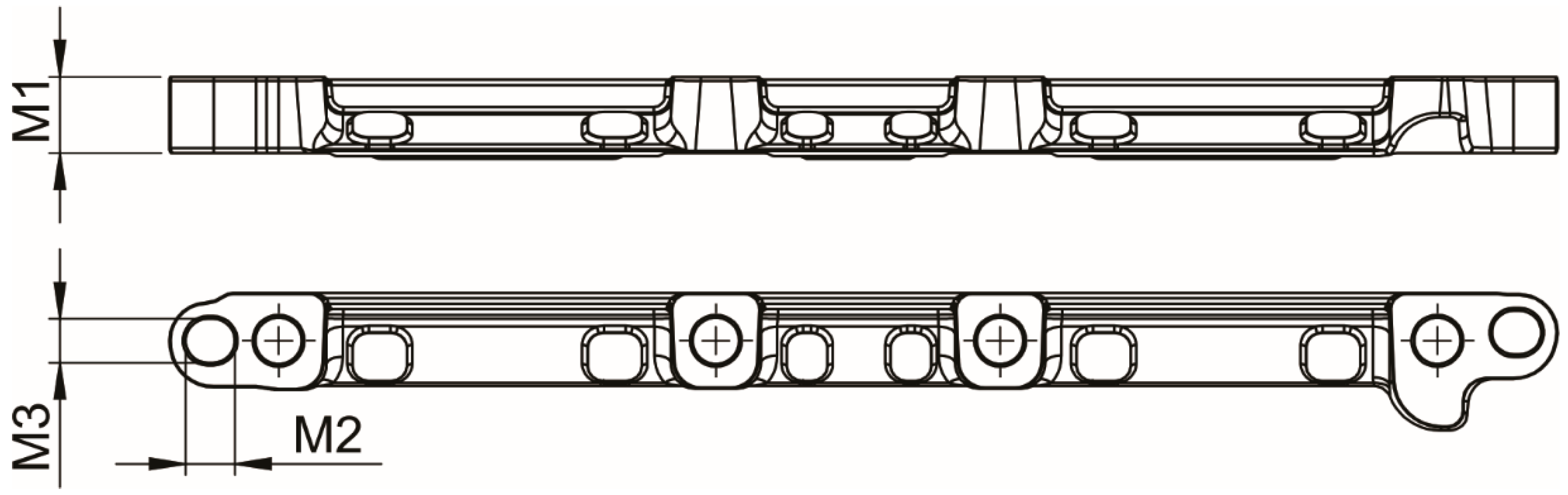
| M1—part’s thickness | The probe is directed downwards, with a low probability of residue accumulation. | Keyence GT2-A32 |
| M2—hole length | The probe is installed horizontally; its tip is protected by the cover. | Keyence GT2-PA12 |
| M3—hole width | The probe is installed horizontally; its tip is occluded by the casing of a measuring rod. | Keyence GT2-PA12 |
| Parameter | Description | Unit | |
|---|---|---|---|
| Process parameters | TIME | Absolute time | / |
| EXT_ID | Fixture table identification number | / | |
| SUB_PROGRAM | Current CNC subprogram | / | |
| CODE_LINE_NUMBER | Current line number in the subprogram | / | |
| Motor parameters | FEED_RATE | Feed rate | mm/min |
| SPINDLE_SPEED_S1 | Rotational velocity of spindle S1 | min−1 | |
| SPINDLE_SPEED_S2 | Rotational velocity of spindle S2 | min−1 | |
| SPINDLE_LOAD_S1 | Torque on the spindle S1, expressed in el. current | A | |
| SPINDLE_LOAD_S2 | Torque on the spindle S2, expressed in el. current | A | |
| SERVO_LOAD_CURRENT_X | el. current in the motor for X axis | A | |
| SERVO_LOAD_CURRENT_Y | el. current in the motor for Y axis | A | |
| SERVO_LOAD_CURRENT_Z | el. current in the motor for Z axis | A | |
| SERVO_LOAD_CURRENT_A | el. current in the motor for A axis | A |
| Parameter | Description | Unit | |
|---|---|---|---|
| Process parameters | TIME | Absolute time | / |
| EXT_ID | Fixture table identification number | / | |
| MEASUREMENT_ID | Identification number of parts on the fixture table in sequence | / | |
| Machined part measurements | M1 | Part thickness | mm |
| M2 | Hole length | mm | |
| M3 | Hole width | mm |
| Function | Nr. of Datapoints | Nr. of Parts | Ratio (Nr. of Parts/All Parts) |
|---|---|---|---|
| min | 68 | 2 | 0.01% |
| max | 322 | 2 | 0.01% |
| average | 229 | 0 | 0.00% |
| median | 230 | 1418 | 9.56% |
| modus | 231 | 1634 | 11.01% |
| ML Algorithm | Fixed Hyper-Parameters | Grid Searched Hyper-Parameters |
|---|---|---|
| RF | ccp_alpha: 0.0, criterion: squared error, max_features: 1.0, max_leaf_nodes: None, max_samples: None, min_impurity_decrease: 0.0, min_samples_leaf: 1, min_samples_split: 2, min_weight_fraction_leaf: 0.0, oob_score: False, random_state: 54, warm_start: False | |
| k-NN | Algorithm: auto, metric: minkowski, metric_params: None, p: 2 | |
| DT | ccp_alpha: 0.0, criterion: squared error, max_features: None, max_leaf_nodes: None, min_impurity_decrease: 0.0, min_samples_leaf: 1, min_samples_split: 2, min_weight_fraction_leaf: 0.0, random_state: 54, warm_start: False |
| Feature Extraction Algorithm | ML Algorithm | Best Grid Searched Hyper-Parameters | Mean Test MAPE | Mean Train MAPE | |
|---|---|---|---|---|---|
| M1—machined part measurement | Tsfresh | RF | 0.003455 | 0.003234 | |
| k-NN | 0.003731 | 0.003349 | |||
| DT | 0.003474 | 0.002823 | |||
| ROCKET | RF | 0.003535 | 0.003029 | ||
| k-NN | 0.003755 | 0.003276 | |||
| DT | 0.003595 | 0.002783 |
| Feature Extraction Algorithm | ML Algorithm | Best Grid Searched Hyper-Parameters | Mean Test MAPE | Mean Train MAPE | |
|---|---|---|---|---|---|
| M2—machined part measurement | Tsfresh | RF | 0.006378 | 0.006109 | |
| k-NN | 0.006765 | 0.006049 | |||
| DT | 0.006369 | 0.006144 | |||
| ROCKET | RF | 0.006550 | 0.006102 | ||
| k-NN | 0.006760 | 0.005999 | |||
| DT | 0.006930 | 0.006163 |
| Feature Extraction Algorithm | ML Algorithm | Best Grid-Searched Hyper-Parameters | Mean Test MAPE | Mean Train MAPE | |
|---|---|---|---|---|---|
| M3—machined part measurement | Tsfresh | RF | 0.003337 | 0.002753 | |
| k-NN | 0.003571 | 0.002914 | |||
| DT | 0.003325 | 0.002775 | |||
| ROCKET | RF | 0.003626 | 0.002629 | ||
| k-NN | 0.003457 | 0.002837 | |||
| DT | 0.003443 | 0.002814 |
| Machined Part Measurements | ML Algorithm | Best Grid-Searched Hyper-Parameters | Mean Test MSE | Mean Train MSE | Mean Test ME | Mean Train ME |
|---|---|---|---|---|---|---|
| M1 | RF | 0.013185 | 0.004093 | 1.070290 | 1.422961 | |
| M2 | DT | 0.022739 | 0.008752 | 1.125031 | 2.664294 | |
| M3 | DT | 0.022985 | 0.007967 | 1.333249 | 0.114721 |
Disclaimer/Publisher’s Note: The statements, opinions and data contained in all publications are solely those of the individual author(s) and contributor(s) and not of MDPI and/or the editor(s). MDPI and/or the editor(s) disclaim responsibility for any injury to people or property resulting from any ideas, methods, instructions or products referred to in the content. |
© 2024 by the authors. Licensee MDPI, Basel, Switzerland. This article is an open access article distributed under the terms and conditions of the Creative Commons Attribution (CC BY) license (https://creativecommons.org/licenses/by/4.0/).
Share and Cite
Berus, L.; Hernavs, J.; Potocnik, D.; Sket, K.; Ficko, M. Enhancing Manufacturing Precision: Leveraging Motor Currents Data of Computer Numerical Control Machines for Geometrical Accuracy Prediction Through Machine Learning. Sensors 2025, 25, 169. https://doi.org/10.3390/s25010169
Berus L, Hernavs J, Potocnik D, Sket K, Ficko M. Enhancing Manufacturing Precision: Leveraging Motor Currents Data of Computer Numerical Control Machines for Geometrical Accuracy Prediction Through Machine Learning. Sensors. 2025; 25(1):169. https://doi.org/10.3390/s25010169
Chicago/Turabian StyleBerus, Lucijano, Jernej Hernavs, David Potocnik, Kristijan Sket, and Mirko Ficko. 2025. "Enhancing Manufacturing Precision: Leveraging Motor Currents Data of Computer Numerical Control Machines for Geometrical Accuracy Prediction Through Machine Learning" Sensors 25, no. 1: 169. https://doi.org/10.3390/s25010169
APA StyleBerus, L., Hernavs, J., Potocnik, D., Sket, K., & Ficko, M. (2025). Enhancing Manufacturing Precision: Leveraging Motor Currents Data of Computer Numerical Control Machines for Geometrical Accuracy Prediction Through Machine Learning. Sensors, 25(1), 169. https://doi.org/10.3390/s25010169