
Deep Neural Network-Based Phase-Modulated Continuous-Wave LiDAR


 ,
,  ,
, 
 ,
, 


Abstract
1. Introduction
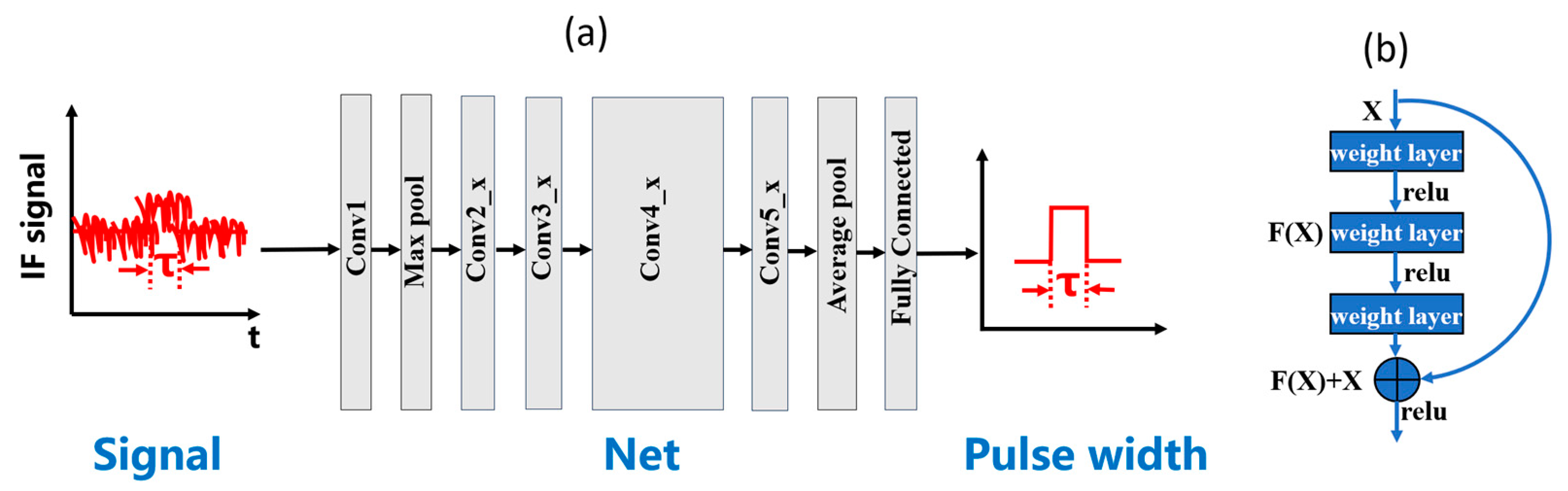
2. Analysis
3. Experimental Section and Results
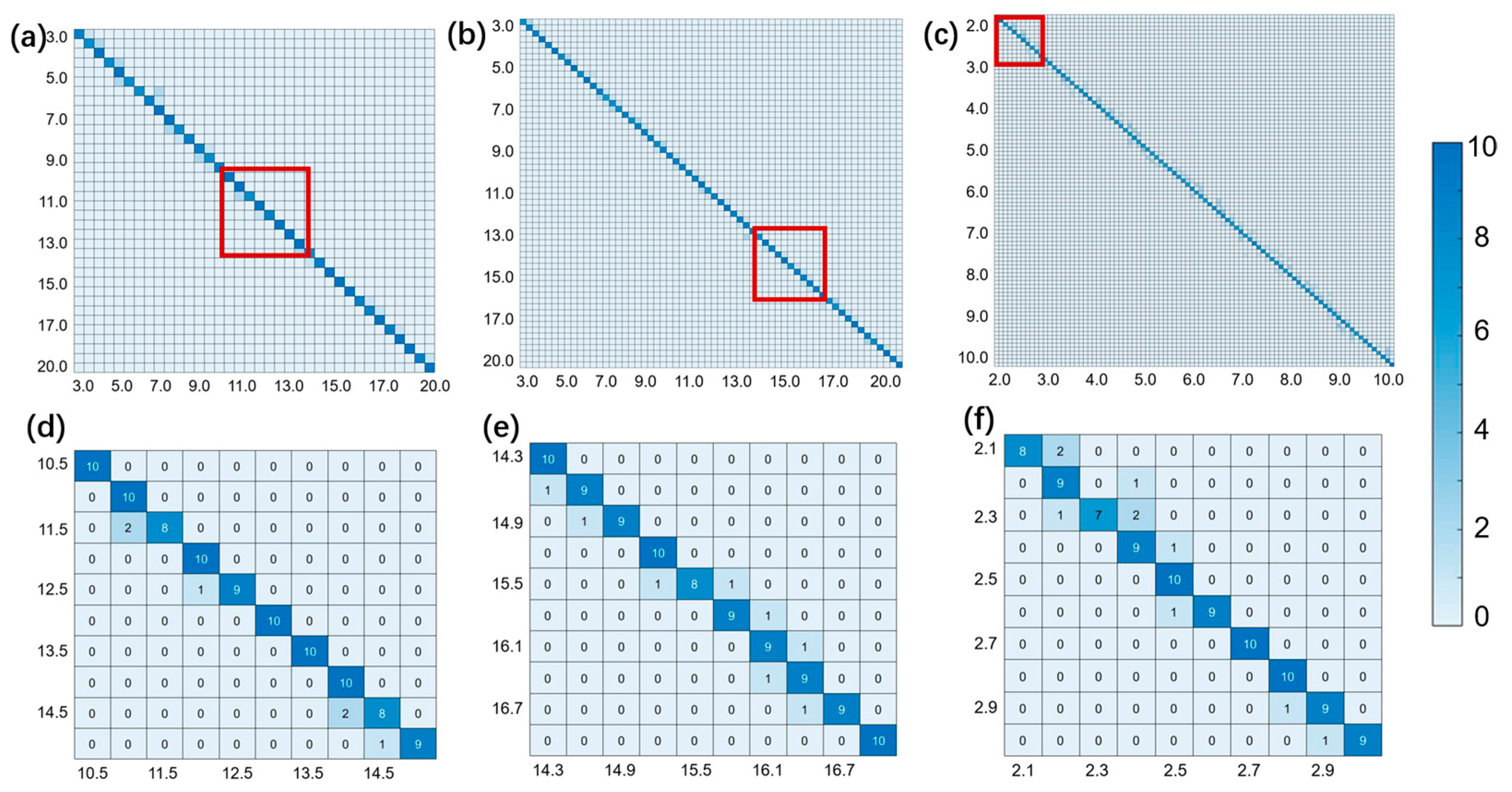
3.1. Influence of Resolution on Network Accuracy
3.2. Influence of SNR on Network Accuracy
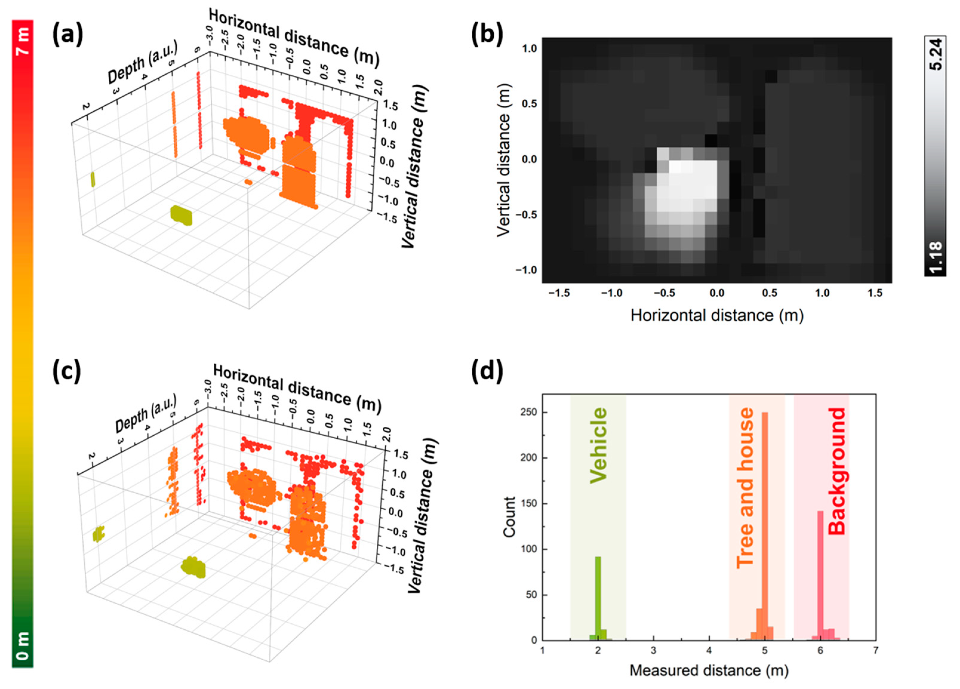
3.3. Point Cloud Imaging Demonstration
4. Conclusions
Author Contributions
Funding
Institutional Review Board Statement
Informed Consent Statement
Data Availability Statement
Conflicts of Interest
References
- Behroozpour, B.; Sandborn, P.A.M.; Wu, M.C.; Boser, B.E. Lidar System Architectures and Circuits. IEEE Commun. Mag. 2017, 55, 135–142. [Google Scholar] [CrossRef]
- Hu, M.; Pang, Y.; Gao, L. Advances in Silicon-Based Integrated Lidar. Sensors 2023, 23, 5920. [Google Scholar] [CrossRef] [PubMed]
- Li, N.; Ho, C.P.; Xue, J.; Lim, L.W.; Chen, G.; Fu, Y.H.; Lee, L.Y.T. A Progress Review on Solid-State LiDAR and Nanophotonics-Based LiDAR Sensors. Laser Photonics Rev. 2022, 16, 2100511. [Google Scholar] [CrossRef]
- Hyun, L.J. Three Dimensional Lidar System Comprises 3D Lidar Scan Unit Mounted on Drones, Autonomous Vehicles and Manned Aircraft Used to Scan Features and Create Three Dimensional Terrain And Feature Files. Korea Patent KR2021066665-A, 7 June 2021. [Google Scholar]
- Sun, P.P.; Sun, C.H.; Wang, R.M.; Zhao, X.M. Object Detection Based on Roadside LiDAR for Cooperative Driving Automation: A Review. Sensors 2022, 22, 9316. [Google Scholar] [CrossRef] [PubMed]
- Na, Q.; Xie, Q.; Zhang, N.; Zhang, L.; Li, Y.; Chen, B.; Peng, T.; Zuo, G.; Zhuang, D.; Song, J. Optical frequency shifted FMCW Lidar system for unambiguous measurement of distance and velocity. Opt. Lasers Eng. 2023, 164, 107523. [Google Scholar] [CrossRef]
- Yoon, J.; Yoon, H.; Kim, J.-Y.; Kim, J.; Kang, G.; Kwon, N.-H.; Kurt, H.; Park, H.-H. Demonstration of High-Accuracy 3D Imaging Using a Si Optical Phased Array with a Tunable Radiator. Opt. Express 2023, 31, 9935–9944. [Google Scholar] [CrossRef] [PubMed]
- Pacala, A.; Yu, T.; Eldada, L. Time-of-Flight (ToF) Lidar Ranging Apparatus for Real-Time Three-Dimensional Mapping and Object Detection, has Processing Electronics that Combines Two Dimensional Scan Data Originating at Optical Antenna Array with Time of Flight Data. U.S. Patent 11209546-B1, 8 December 2021. [Google Scholar]
- Herman, D.M.; Lesky, A.; Beras, R.; Arunmozhi, A. Method for Determining Misalignment of Lidar Sensor Installed in Vehicle e.g. Land Vehicle, Involves Aligning Lidar Sensor Based on Misalignment of Frequency Modulated Continuous Wave (FMCW) Lidar Sensor, and Operating Vehicle Based on Aligned FMCW Lidar Sensor. Germany Patent DE102021103774-A1, 17 February 2021. [Google Scholar]
- Zhang, X.; Pouls, J.; Wu, M.C. Laser frequency sweep linearization by iterative learning pre-distortion for FMCW LiDAR. Opt. Express 2019, 27, 9965–9974. [Google Scholar] [CrossRef] [PubMed]
- Zhang, J.; Liu, C.; Su, L.; Fu, X.; Jin, W.; Bi, W.; Fu, G. Wide range linearization calibration method for DFB Laser in FMCW LiDAR. Opt. Lasers Eng. 2024, 174, 107961. [Google Scholar] [CrossRef]
- Kamata, M.; Hinakura, Y.; Baba, T. Carrier-Suppressed Single Sideband Signal for FMCW LiDAR Using a Si Photonic-Crystal Optical Modulators. J. Light. Technol. 2020, 38, 2315–2321. [Google Scholar] [CrossRef]
- Shi, P.; Lu, L.; Liu, C.; Zhou, G.; Xu, W.; Chen, J.; Zhou, L. Optical FMCW Signal Generation Using a Silicon Dual-Parallel Mach-Zehnder Modulator. IEEE Photonics Technol. Lett. 2021, 33, 301–304. [Google Scholar] [CrossRef]
- Mingshi, Z.; Yubing, W.; Lanxuan, Z.; Qian, H.; Shuhua, Z.; Lei, L.; Yongyi, C.; Li, Q.; Junfeng, S.; Lijun, W. Phase-modulated continuous-wave coherent ranging method for optical phased array lidar. Opt. Express 2023, 31, 6514–6528. [Google Scholar] [CrossRef] [PubMed]
- An, Y.; Guo, J. High Precision Time Digital Converter for Resisting Pulse Width Modulation (PVT) Change, has Numerical Control Annular Vernier Time-to-Digital Converter (TDC) Module Whose Output End is Connected with Input End of Result Calculating Module. Chinese Patent CN114967409-A, 28 March 2022. [Google Scholar]
- Varlik, A.; Uray, F. Filtering airborne LIDAR data by using fully convolutional networks. Surv. Rev. 2023, 55, 21–31. [Google Scholar] [CrossRef]
- Yan, Y.; Yan, H.; Guo, J.; Dai, H. Classification and Segmentation of Mining Area Objects in Large-Scale Spares Lidar Point Cloud Using a Novel Rotated Density Network. Isprs Int. J. Geo-Inf. 2020, 9, 182. [Google Scholar] [CrossRef]
- Yu, J.; Zhang, F.; Chen, Z.; Liu, L. MSPR-Net: A Multi-Scale Features Based Point Cloud Registration Network. Remote Sens. 2022, 14, 4874. [Google Scholar] [CrossRef]
- Fan, J.; Lian, T. Youtube Data Analysis using Linear Regression and Neural Network. In Proceedings of the 2022 International Conference on Big Data, Information and Computer Network (BDICN), Sanya, China, 20–22 January 2022; pp. 248–251. [Google Scholar]
- Ma, X.; Tang, Z.; Xu, T.; Yang, L.; Wang, Y. Method for Performing Sensor Physical Quantity Regression Process Based on ICS-BP Neural Network, Involves Training Neural Network Using Trained Neural Network Regression Prediction to Physical Quantity of Sensor. Chinese Patent CN115034361-A, 2 June 2022. [Google Scholar]
- Yang, Y.; Yao, Q.; Wang, Y. Identifying Generalized Regression Neural Network Acoustic Signal Using Mel Frequency Cepstral Coefficient Involves Extracting Mel Frequency Cepstral Coefficient Features, and Analyzing Identification Performance of Generalized Regression Neural Network Model. Chinese Patent CN115331678-A, 11 November 2022. [Google Scholar]
- Morrison, R.A.; Turner, J.T.; Barwick, M.; Hardaway, G.M. Urban reconnaissance with an ultra high resolution ground vehicle mounted laser radar. In Proceedings of the Conference on Laser Radar Technology and Applications X, Orlando, FL, USA, 19 May 2005. [Google Scholar]
- Shiina, T.; Yamada, S.; Senshu, H.; Otobe, N.; Hashimoto, G.; Kawabata, Y. LED Mini-Lidar for Mars Rover. In Proceedings of the Conference on Lidar Technologies, Techniques, and Measurements for Atmospheric Remote Sensing XII, Edinburgh, UK, 24 October 2016. [Google Scholar]
- Zaremotekhases, F.; Hunsaker, A.; Dave, E.V.V.; Sias, J.E.E. Performance of the UAS-LiDAR sensing approach in detecting and measuring pavement frost heaves. Road Mater. Pavement Des. 2024, 25, 308–325. [Google Scholar] [CrossRef]
- Feng, H.; Pan, L.; Yang, F.; Pei, H.; Wang, H.; Yang, G.; Liu, M.; Wu, Z. Height and Biomass Inversion of Winter Wheat Based on Canopy Height Model. In Proceedings of the 38th IEEE International Geoscience and Remote Sensing Symposium (IGARSS), Valencia, Spain, 22–27 July 2018; pp. 7711–7714. [Google Scholar]
- Yuan, Q.-Y.; Niu, L.-H.; Hu, C.-C.; Wu, L.; Yang, H.-R.; Yu, B. Target Reconstruction of Streak Tube Imaging Lidar Based on Gaussian Fitting. Acta Photonica Sin. 2017, 46, 1211002. [Google Scholar] [CrossRef]
- Su, J.; Su, H.; Wang, D.; Gan, W. Multi-Task Behavior Recognition Model Training Method, Involves Obtaining Multiple Classification Networks Corresponding to to-be-Identified Task, and Obtaining Classification Networks by Training Classification Networks. Chinese Patent CN113344048-A, 3 September 2021. [Google Scholar]
- Yin, J.; Li, Q.; Huang, J.; Wang, T.; Ren, Y.; Cui, C. Method for Training Classification Network, Involves Obtaining Classification Result for Representing Type of Airway, and Adjusting Parameters of Classification Network Based on Classification Result. Chinese Patent CN115222834-A, 21 October 2022. [Google Scholar]
- Zhang, Y.; Lu, L.; Wang, S.; Wu, H.; Tang, M. Method for Training Interaction Text Classification in Natural Language Processing Fields, Involves Performing Multi-Task Training on Classification Training Networks until Preset Classification Network Satisfies Preset Conditions to Obtain Target Classification Network as Text Classification Model. Chinese Patent CN116932744-A, 24 October 2023. [Google Scholar]
- He, K.; Zhang, X.; Ren, S.; Sun, J. Deep residual learning for image recognition. In Proceedings of the IEEE Conference on Computer Vision and Pattern Recognition, Las Vegas, NV, USA, 27–30 June 2016; pp. 770–778. [Google Scholar]
- Krizhevsky, A.; Sutskever, I.; Hinton, G.E. Imagenet classification with deep convolutional neural networks. Adv. Neural Inf. Process. Syst. 2012, 25. [Google Scholar] [CrossRef]
- LeCun, Y.; Bottou, L.; Bengio, Y.; Haffner, P.J.P. Gradient-based learning applied to document recognition. Proc. IEEE 1998, 86, 2278–2324. [Google Scholar] [CrossRef]
- Simonyan, K.; Zisserman, A. Very deep convolutional networks for large-scale image recognition. arXiv 2014, arXiv:1409.1556. [Google Scholar]
- Szegedy, C.; Liu, W.; Jia, Y.; Sermanet, P.; Reed, S.; Anguelov, D.; Erhan, D.; Vanhoucke, V.; Rabinovich, A. Going deeper with convolutions. In Proceedings of the IEEE Conference on Computer Vision and Pattern Recognition, Boston, MA, USA, 7–12 June 2015; pp. 1–9. [Google Scholar]
- Poulton, C.V.; Yaacobi, A.; Cole, D.B.; Byrd, M.J.; Raval, M.; Vermeulen, D.; Watts, M.R. Coherent solid-state LIDAR with silicon photonic optical phased arrays. Opt. Lett. 2017, 42, 4091–4094. [Google Scholar] [CrossRef]


| Resolution (m) | Distance Range (m) | No. of Class | Total Training Quantity | Testing Quantity | Accuracy % |
|---|---|---|---|---|---|
| 0.5 | 2.8–20.7 | 36 | 4000 | 360 | 97.8 |
| 0.4 | 2.8–20.7 | 45 | 5000 | 450 | 95.4 |
| 0.3 | 2.8–20.7 | 60 | 6000 | 600 | 93.6 |
| 0.2 | 1.8–10.7 | 45 | 5000 | 450 | 92.9 |
| 0.1 | 1.8–10.7 | 90 | 10,000 | 900 | 90.2 |
| Signal-to-Noise Ratio | Accuracy % |
|---|---|
| 20 | 90.2 |
| 15 | 84.6 |
| 10 | 85.3 |
| 5 | 82.2 |
| 2 | 81.4 |
Disclaimer/Publisher’s Note: The statements, opinions and data contained in all publications are solely those of the individual author(s) and contributor(s) and not of MDPI and/or the editor(s). MDPI and/or the editor(s) disclaim responsibility for any injury to people or property resulting from any ideas, methods, instructions or products referred to in the content. |
© 2024 by the authors. Licensee MDPI, Basel, Switzerland. This article is an open access article distributed under the terms and conditions of the Creative Commons Attribution (CC BY) license (https://creativecommons.org/licenses/by/4.0/).
Share and Cite
Zhang, H.; Wang, Y.; Zhang, M.; Song, Y.; Qiu, C.; Lei, Y.; Jia, P.; Liang, L.; Zhang, J.; Qin, L.; et al. Deep Neural Network-Based Phase-Modulated Continuous-Wave LiDAR. Sensors 2024, 24, 1617. https://doi.org/10.3390/s24051617
Zhang H, Wang Y, Zhang M, Song Y, Qiu C, Lei Y, Jia P, Liang L, Zhang J, Qin L, et al. Deep Neural Network-Based Phase-Modulated Continuous-Wave LiDAR. Sensors. 2024; 24(5):1617. https://doi.org/10.3390/s24051617
Chicago/Turabian StyleZhang, Hao, Yubing Wang, Mingshi Zhang, Yue Song, Cheng Qiu, Yuxin Lei, Peng Jia, Lei Liang, Jianwei Zhang, Li Qin, and et al. 2024. "Deep Neural Network-Based Phase-Modulated Continuous-Wave LiDAR" Sensors 24, no. 5: 1617. https://doi.org/10.3390/s24051617
APA StyleZhang, H., Wang, Y., Zhang, M., Song, Y., Qiu, C., Lei, Y., Jia, P., Liang, L., Zhang, J., Qin, L., Ning, Y., & Wang, L. (2024). Deep Neural Network-Based Phase-Modulated Continuous-Wave LiDAR. Sensors, 24(5), 1617. https://doi.org/10.3390/s24051617