

Multi-Hop Clustering and Routing Protocol Based on Enhanced Snake Optimizer and Golden Jackal Optimization in WSNs

Abstract
1. Introduction
- (1)
- The ESO-GJO method adds a Brownian motion function to the SO algorithm’s exploitation stage in order to avoid local optima.
- (2)
- The proposed approach uses SO to select the optimal CHs and considers variables such as energy and distance when building the fitness function.
- (3)
- The suggested algorithm uses GJO to determine the route from CH to BS and initializes the GJO population through backward learning.
- Section 2: Summarizes previous work in related fields.
- Section 3: Introduces the energy model and network model.
- Section 4: Offers a detailed introduction to the algorithm proposed in this article.
- Section 5: Performance metrics simulation demonstration and comparison.
- Section 6: Summarizes the research work in this paper and suggests future work to be carried out.
2. Related Works
3. Preliminaries
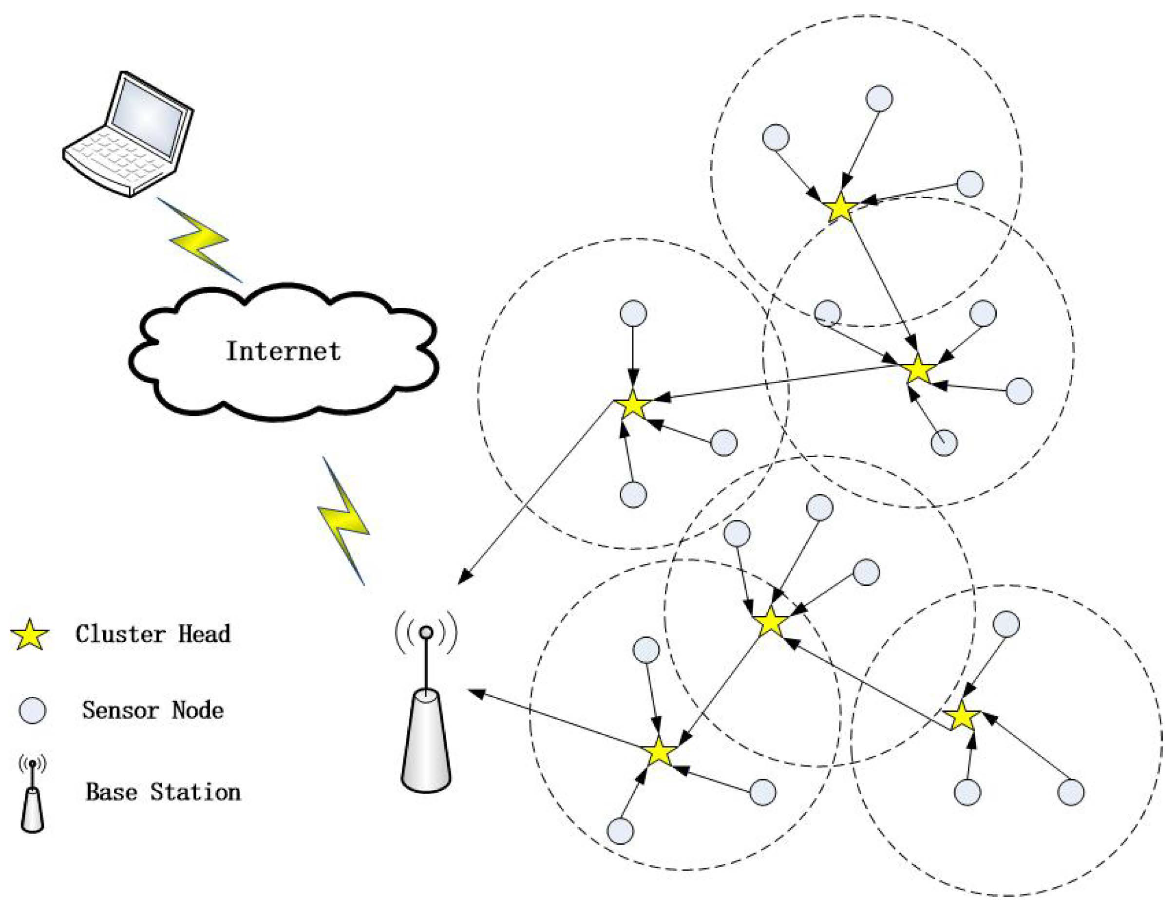
3.1. Network Model
- In WSNs, every sensor node has the same initial energy.
- Distances between nodes are calculated using Euclidean distance.
- Within the sensing area, sensor nodes are haphazardly placed and maintain a fixed location once deployed.
- The BS can be positioned either within or outside the screening region, and it remains stationary.
- The sensor node as a cluster member transmits the collected environmental data to the CH.
- The aggregated data are transferred to the BS via CH.
3.2. Energy Model
4. Proposed Method
4.1. CH Selection Stage
4.1.1. CH Selection Using SO
4.1.2. Fitness Function of SO
- (1)
- Energy consumption of CH:This is the first parameter of the fitness function. Our goal is to prioritize nodes with low energy consumption as CH. Let represent the ’s energy consumption, and assume that , K is the number of CHs.Consequently, minimizing the objective function is our aim:
- (2)
- Distance between node and BS:This is the second parameter of the fitness function. Our goal is to prioritize the node with the shortest distance to the common node and BS as the CH. Let be the distance from intra-cluster node to cluster head node . Let be the distance from to BS where , K represents the quantity of CHs and , M represents the quantity of cluster members. Consequently, minimizing the objective function is our aim:
- (3)
- Node Degree of CH: This is the third parameter of the fitness function. High-degree nodes are given preference to become CH in the ESO-GJO CH selection process. Consequently, our goal is to maximize the objective function as follows
4.2. Data Routing Stage
4.2.1. Routing Algorithm Using GJO
- (1)
- The stage of exploration or hunting for preyThis section proposes GJO’s exploration plan. Jackals can sense and follow their prey due to their innate instincts, yet sometimes the prey escapes and is hard to catch. As a result, the females follow the males and lead the pack in search of additional prey.where t is the current iteration. represents the prey’s position vector, while and represent the locations of the male and female jackals. The updated positions of the male and female jackals with respect to the prey are shown by and .The prey’s initial energy level is represented by , while its decreasing energy is represented by .where r can be any integer between 0 and 1.where ; the rounds of iteration are denoted by T and is calculated by Equation (36):
- (2)
- The stage of exploitation or encircling and leaping for preyThe mathematical model of joint roundup of male and female jackals is shown in Equations (39) and (40):
4.2.2. Fitness Function of GJO
- (1)
- Distance between CH and BS: The further the distance between the CH and the BS, the more energy is required to transmit the data. Therefore, the CH close to the BS is selected to form the best path. Consequently, minimizing the objective function is our aim:
- (2)
- The ratio of the distance between CH and BS to the inter-cluster head distance:The fitness function’s second parameter will be this ratio. Here, maximizing the inter-cluster distance and minimizing the distance between and BS are the main objectives. Consequently, minimizing the objective function is our aim:
- (3)
- Residual energy of CH: This is the fitness function’s third parameter. Our goal is to prioritize the CH with more remaining energy as the next hop. Let denote the residual energy of CH; K denotes the number of CHs. Consequently, our goal is to maximize the objective function as follows:The following three functions , , and , are to be minimized as the fitness function for our suggested GJO method. As a result, the following is the fitness function for our algorithm:where , , and are constants that give the objective functions weights. The total of these constants ought to equal 1. Minimizing the objective function is our aim.
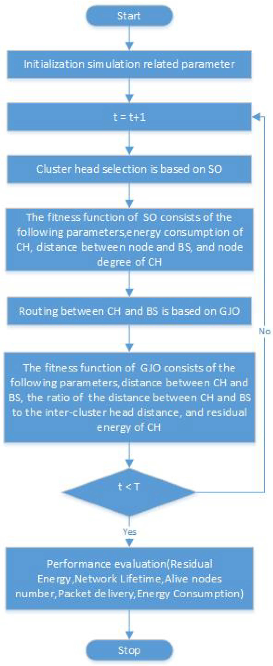
4.3. The Pseudo-Code of the Proposed Algorithm
| Algorithm 1 SO-Clustering |
|
| Algorithm 2 GJO-Routing |
|
5. Simulation Results
5.1. Simulation Settings
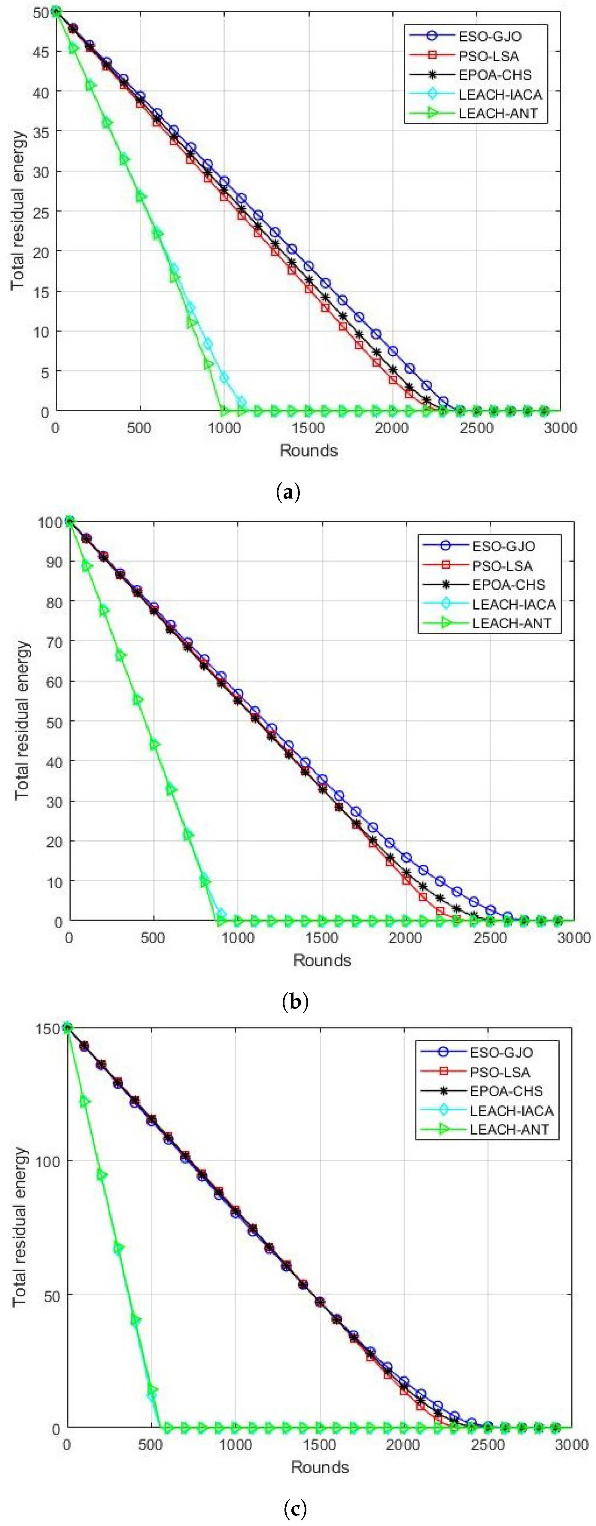
5.2. Residual Energy
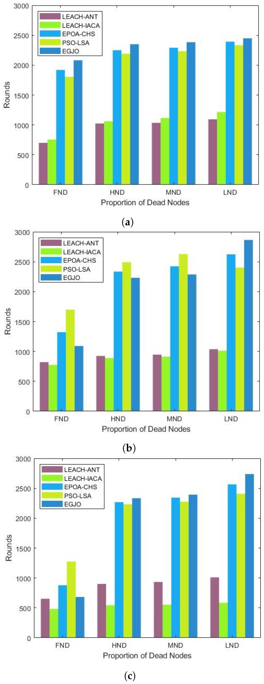
5.3. Network Lifetime
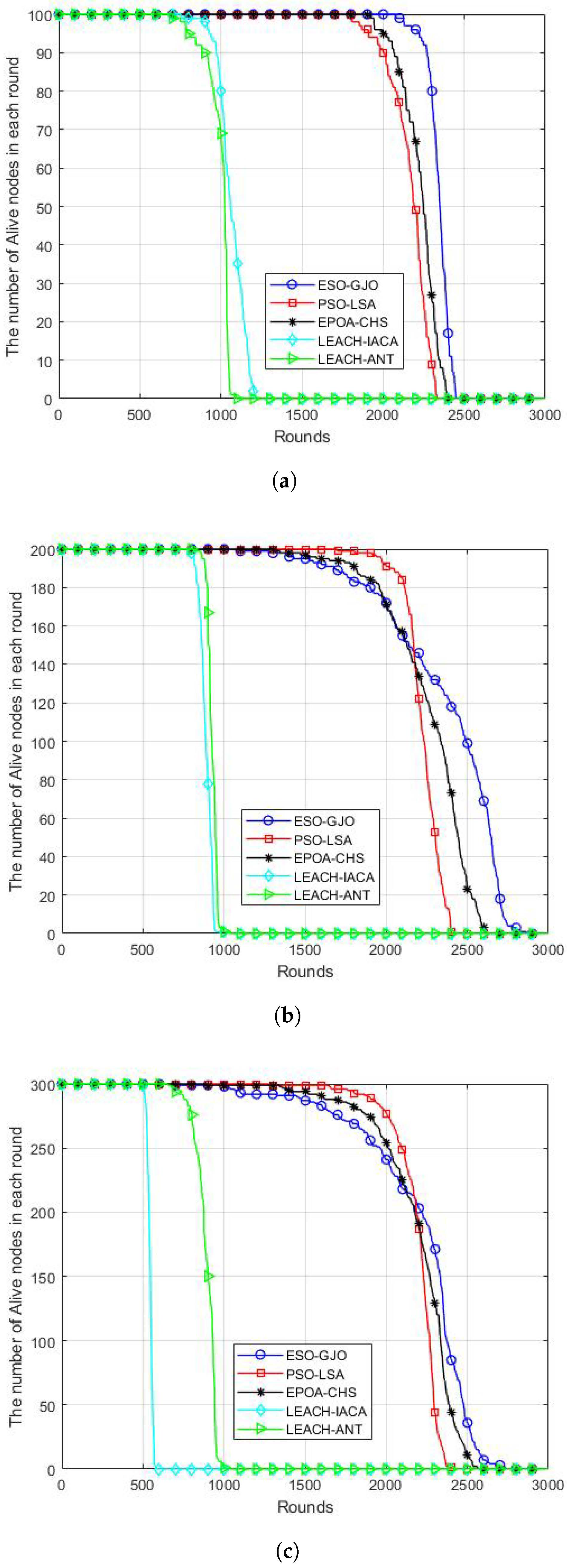
5.4. Live Nodes Number
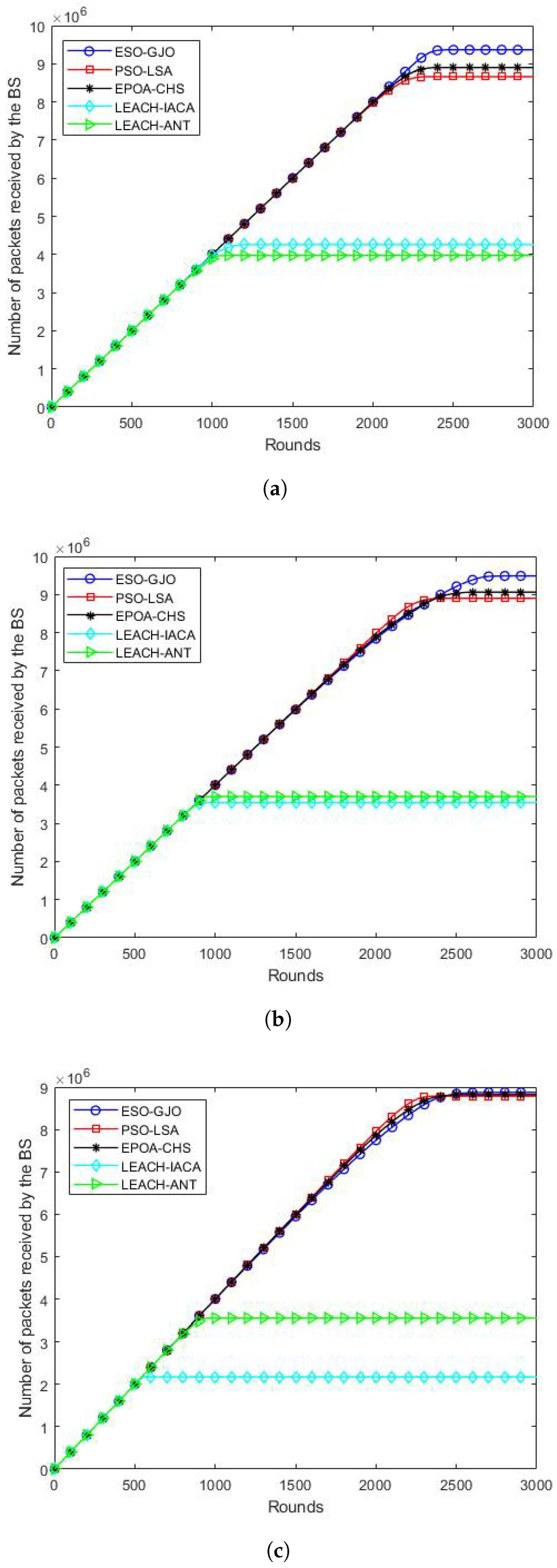
5.5. Packet Delivery


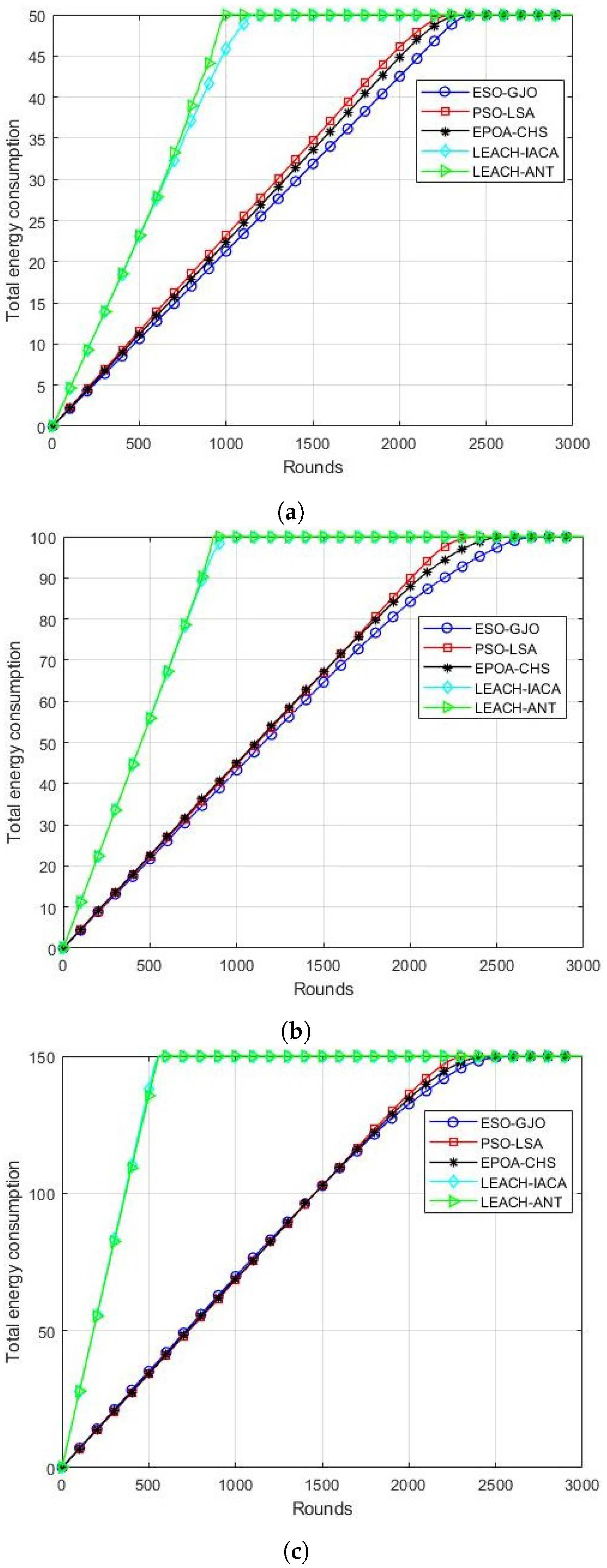
5.6. Energy Consumption
6. Conclusions
Author Contributions
Funding
Institutional Review Board Statement
Informed Consent Statement
Data Availability Statement
Conflicts of Interest
References
- Fischione, C. An Introduction to Wireless Sensor Networks; KTH Royal Institute of Technology: Stockholm, Sweden, 2014. [Google Scholar]
- BenSaleh, M.S.; Saida, R.; Kacem, Y.H.; Abid, M. Wireless Sensor Network Design Methodologies: A Survey. J. Sens. 2020, 2020, 9592836. [Google Scholar] [CrossRef]
- Kandris, D.; Nakas, C.; Vomvas, D.; Koulouras, G. Applications of wireless sensor networks: An up-to-date survey. Appl. Syst. Innov. 2020, 3, 14. [Google Scholar] [CrossRef]
- Aranda, J.; Mendez, D.; Carrillo, H. Multimodal wireless sensor networks for monitoring applications: A review. J. Circuits, Syst. Comput. 2020, 29, 2030003. [Google Scholar] [CrossRef]
- Mohamed, R.E.; Saleh, A.I.; Abdelrazzak, M.; Samra, A.S. Survey on wireless sensor network applications and energy efficient routing protocols. Wirel. Pers. Commun. 2018, 101, 1019–1055. [Google Scholar] [CrossRef]
- Priyadarshi, R.; Gupta, B.; Anurag, A. Deployment techniques in wireless sensor networks: A survey, classification, challenges, and future research issues. J. Supercomput. 2020, 76, 7333–7373. [Google Scholar] [CrossRef]
- Amutha, J.; Sharma, S.; Nagar, J. WSN strategies based on sensors, deployment, sensing models, coverage and energy efficiency: Review, approaches and open issues. Wirel. Pers. Commun. 2020, 111, 1089–1115. [Google Scholar] [CrossRef]
- Croce, S.; Marcelloni, F.; Vecchio, M. Reducing power consumption in wireless sensor networks using a novel approach to data aggregation. Comput. J. 2008, 51, 227–239. [Google Scholar] [CrossRef]
- Fanian, F.; Rafsanjani, M.K. Cluster-based routing protocols in wireless sensor networks: A survey based on methodology. J. Netw. Comput. Appl. 2019, 142, 111–142. [Google Scholar] [CrossRef]
- Wang, Q.; Lin, D.; Yang, P.; Zhang, Z. An energy-efficient compressive sensing-based clustering routing protocol for WSNs. IEEE Sens. J. 2019, 19, 3950–3960. [Google Scholar] [CrossRef]
- Shafiq, M.; Ashraf, H.; Ullah, A.; Tahira, S. Systematic Literature Review on Energy Efficient Routing Schemes in WSN—A Survey. Mob. Netw. Appl. 2020, 25, 882–895. [Google Scholar] [CrossRef]
- Nakas, C.; Kandris, D.; Visvardis, G. Energy efficient routing in wireless sensor networks: A comprehensive survey. Algorithms 2020, 13, 72. [Google Scholar] [CrossRef]
- Daniel, A.; Balamurugan, K.M.; Vijay, R.; Arjun, K. Energy aware clustering with multihop routing algorithm for wireless sensor networks. Intell. Autom. Soft Comput. 2021, 29, 233–246. [Google Scholar] [CrossRef]
- Saleem, M.M.; Alabady, S.A. Improvement of the WMSNs lifetime using multi-hop clustering routing protocol. Wirel. Netw. 2022, 28, 3173–3183. [Google Scholar] [CrossRef]
- Pantazis, N.A.; Nikolidakis, S.A.; Vergados, D. Energy-efcient routing protocols in wireless sensor networks: A survey. IEEE Commun. Surv. Tutor. 2013, 15, 551–591. [Google Scholar] [CrossRef]
- Behera, T.M.; Samal, U.C.; Mohapatra, S.K.; Khan, M.S.; Appasani, B.; Bizon, N.; Thounthong, P. Energy-Efficient Routing Protocols for Wireless Sensor Networks: Architectures, Strategies, and Performance. Electronics 2022, 11, 2282. [Google Scholar] [CrossRef]
- Al Aghbari, Z.; Khedr, A.M.; Osamy, W.; Arif, I.; Agrawal, D.P. Routing in wireless sensor networks using optimization techniques: A survey. Wirel. Pers. Commun. 2020, 111, 2407–2434. [Google Scholar] [CrossRef]
- Heinzelman, W.R.; Chandrakasan, A.; Balakrishnan, H. Energy-efficient commu nication protocol for wireless microsensor networks. In Proceedings of the 33rd Annual Hawaii International Conference on System Sciences, Maui, HI, USA, 7 January 2000; Volume 1, p. 10. [Google Scholar]
- Liao, Q.; Zhu, H. An Energy Balanced Clustering Algorithm Based on LEACH Protocol. Appl. Mech. Mater. 2013, 341–342, 1138–1143. [Google Scholar] [CrossRef]
- Jerbi, W.; Guermazi, A.; Trabelsi, H. O-LEACH of routing protocol for wireless sensor networks. In Proceedings of the 13th International Conference Computer Vision Graphics and Image Processing (CGiV), Beni Mellal, Morocco, 29 March–1 April 2016; pp. 399–404. [Google Scholar]
- Neto, J.H.B.; Cardoso, A.R.; Celestino, J., Jr. MH-LEACH: A Distributed Algorithm for Multi-Hop Communication. Wirel. Sens. Netw. 2014, 2014, 55–61. [Google Scholar]
- Long, C.; Liao, S.; Zou, X.; Zhou, X.; Zhang, N. An improved LEACH multi-hop routing protocol based on intelligent ant colony algorithm for wireless sensor networks. J. Inf. Comput. Sci. 2014, 11, 2747–2757. [Google Scholar] [CrossRef]
- Agarwal, T.; Kumar, D.; Prakash, N.R. Prolonging Network Lifetime Using Ant Colony Optimization Algorithm on LEACH Protocol for Wireless Sensor Networks; Springer: Berlin/Heidelberg, Germany, 2010; pp. 634–641. [Google Scholar]
- Natesan, G.; Konda, S.; de Prado, R.P.; Wozniak, M. A Hybrid Mayfly-Aquila Optimization Algorithm Based Energy-Efficient Clustering Routing Protocol for Wireless Sensor Networks. Sensors 2022, 22, 6405. [Google Scholar] [CrossRef]
- Yao, Y.; Xie, D.; Li, Y.; Wang, C.; Li, Y. Routing Protocol for Wireless Sensor Networks Based on Archimedes Optimization Algorithm. IEEE Sens. J. 2022, 22, 15561–15573. [Google Scholar] [CrossRef]
- Wang, Z.; Duan, J.; Xu, H.; Song, X.; Yang, Y. Enhanced Pelican Optimization Algorithm for Cluster Head Selection in Heterogeneous Wireless Sensor Networks. Sensors 2023, 23, 7711. [Google Scholar] [CrossRef] [PubMed]
- Punithavathi, R.; Kurangi, C.; Balamurugan, S.P.; Pustokhina, I.V.; Pustokhin, D.A.; Shankar, K. Hybrid BWO-IACO algorithm for cluster based routing in wireless sensor networks. Comput. Mater. Contin. 2021, 69, 433–449. [Google Scholar] [CrossRef]
- Vinitha, A.; Rukmini, M.S.S.; Sunehra, D. Energy-efficient multihop routing in WSN using the hybrid optimization algorithm. Int. J. Commun. Syst. 2020, 33, e4440. [Google Scholar] [CrossRef]
- Senthil, G.A.; Raaza, A.; Kumar, N. Internet of Things Energy Efficient Cluster-Based Routing Using Hybrid Particle Swarm Optimization for Wireless Sensor Network. Wirel. Pers. Commun. 2021, 122, 2603–2619. [Google Scholar] [CrossRef]
- Mantri, D.; Prasad, N.R.; Prasad, R. Grouping of clusters for efficient data aggregation (GCEDA) in wireless sensor network. In Proceedings of the 2013 3rd IEEE International Advance Computing Conference (IACC), Ghaziabad, India, 22–23 February 2013; pp. 132–137. [Google Scholar]
- Sajwan, M.; Gosain, D.; Sharma, A.K. CAMP: Cluster aided multi-path routing protocol for wireless sensor networks. Wirel. Netw. 2019, 25, 2603–2620. [Google Scholar] [CrossRef]
- Hashim, F.A.; Hussien, A.G. Snake Optimizer: A novel meta-heuristic optimization algorithm. Knowl.-Based Syst. 2022, 242, 108320. [Google Scholar] [CrossRef]
- Chopra, N.; Ansari, M.M. Golden jackal optimization: A novel nature-inspired optimizer for engineering applications. Expert Syst. Appl. 2022, 198, 116924. [Google Scholar] [CrossRef]


| Parameters | Value |
|---|---|
| Network Area | 100 × 100, 200 × 200, 300 × 300 (m2) |
| Number of nodes | N = 100, 200, 300 |
| Sink node location | (50 m, 150 m) |
| (100 m, 250 m) | |
| (150 m, 350 m) | |
| 0.5 J | |
| Packet Size | 4000 Bits |
| 50 nJ/bit | |
| 10 nJ/bit/m2 | |
| 0.0013 pJ/bit/m4 | |
| 5 nJ/bit/signal | |
| 70 m |
| No. of Rounds | |||||
|---|---|---|---|---|---|
| Simulation Scenario | Protocol | FND | HND | MND | LND |
| Number of nodes is 100 | ESO-GJO | 2080 | 2350 | 2383 | 2448 |
| PSO-LSA | 1805 | 2191 | 2233 | 2332 | |
| EPOA-CHS | 1920 | 2249 | 2290 | 2392 | |
| LEACH-IACA | 755 | 1060 | 1116 | 1214 | |
| LEACH-ANT | 701 | 1023 | 1035 | 1094 | |
| Number of nodes is 200 | ESO-GJO | 1091 | 2231 | 2287 | 2863 |
| PSO-LSA | 1698 | 2492 | 2628 | 2402 | |
| EPOA-CHS | 1322 | 2334 | 2424 | 2623 | |
| LEACH-IACA | 775 | 889 | 913 | 1012 | |
| LEACH-ANT | 821 | 925 | 947 | 1038 | |
| Number of nodes is 300 | ESO-GJO | 683 | 2333 | 2393 | 2737 |
| PSO-LSA | 1275 | 2230 | 2275 | 2407 | |
| EPOA-CHS | 879 | 2268 | 2343 | 2565 | |
| LEACH-IACA | 483 | 546 | 553 | 584 | |
| LEACH-ANT | 653 | 901 | 934 | 1010 |
Disclaimer/Publisher’s Note: The statements, opinions and data contained in all publications are solely those of the individual author(s) and contributor(s) and not of MDPI and/or the editor(s). MDPI and/or the editor(s) disclaim responsibility for any injury to people or property resulting from any ideas, methods, instructions or products referred to in the content. |
© 2024 by the authors. Licensee MDPI, Basel, Switzerland. This article is an open access article distributed under the terms and conditions of the Creative Commons Attribution (CC BY) license (https://creativecommons.org/licenses/by/4.0/).
Share and Cite
Wang, Z.; Duan, J.; Xing, P. Multi-Hop Clustering and Routing Protocol Based on Enhanced Snake Optimizer and Golden Jackal Optimization in WSNs. Sensors 2024, 24, 1348. https://doi.org/10.3390/s24041348
Wang Z, Duan J, Xing P. Multi-Hop Clustering and Routing Protocol Based on Enhanced Snake Optimizer and Golden Jackal Optimization in WSNs. Sensors. 2024; 24(4):1348. https://doi.org/10.3390/s24041348
Chicago/Turabian StyleWang, Zhen, Jin Duan, and Pengzhan Xing. 2024. "Multi-Hop Clustering and Routing Protocol Based on Enhanced Snake Optimizer and Golden Jackal Optimization in WSNs" Sensors 24, no. 4: 1348. https://doi.org/10.3390/s24041348
APA StyleWang, Z., Duan, J., & Xing, P. (2024). Multi-Hop Clustering and Routing Protocol Based on Enhanced Snake Optimizer and Golden Jackal Optimization in WSNs. Sensors, 24(4), 1348. https://doi.org/10.3390/s24041348