
Low-Cost Optical Sensors for Soil Composition Monitoring


Abstract
1. Introduction
2. Related Work
3. Sensor Proposal
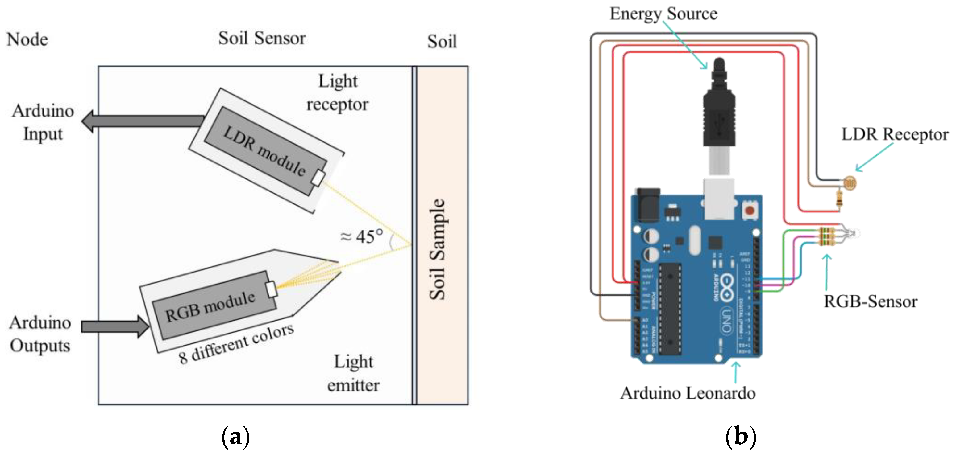
3.1. Sensor Description
3.2. Selected Node
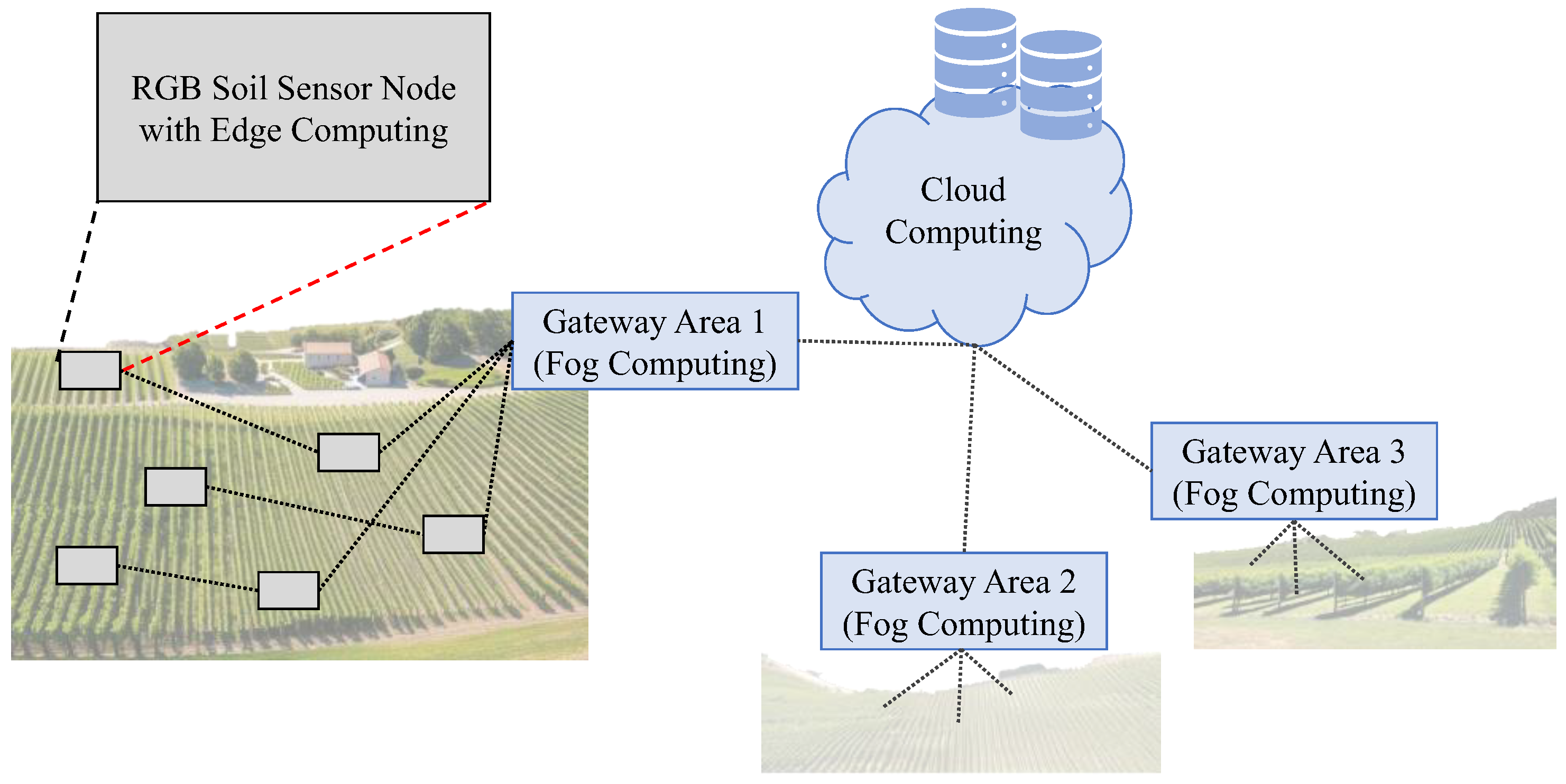
3.3. Architecture
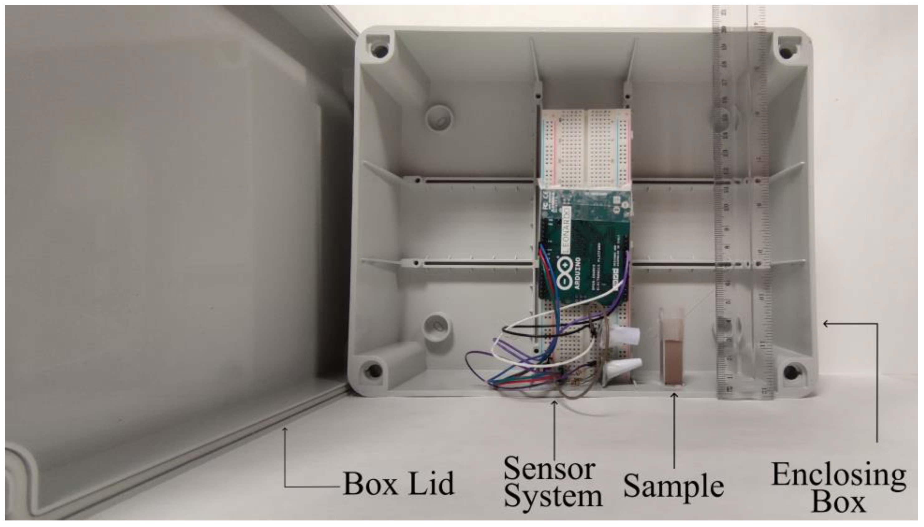
4. Test Bench
4.1. Soil
4.2. Added Substances
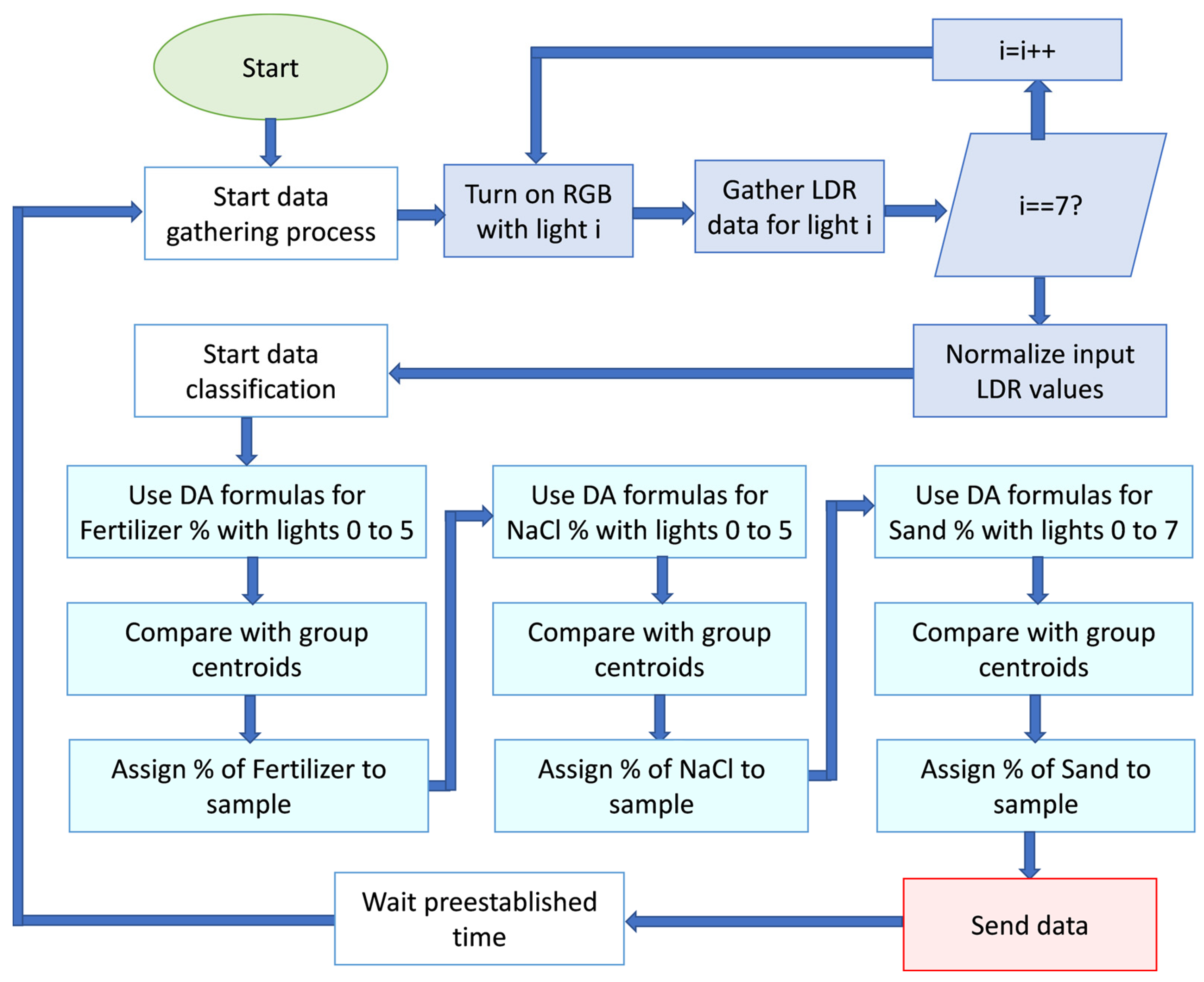
4.3. Data Gathering Process
4.4. Data Processing
5. Results
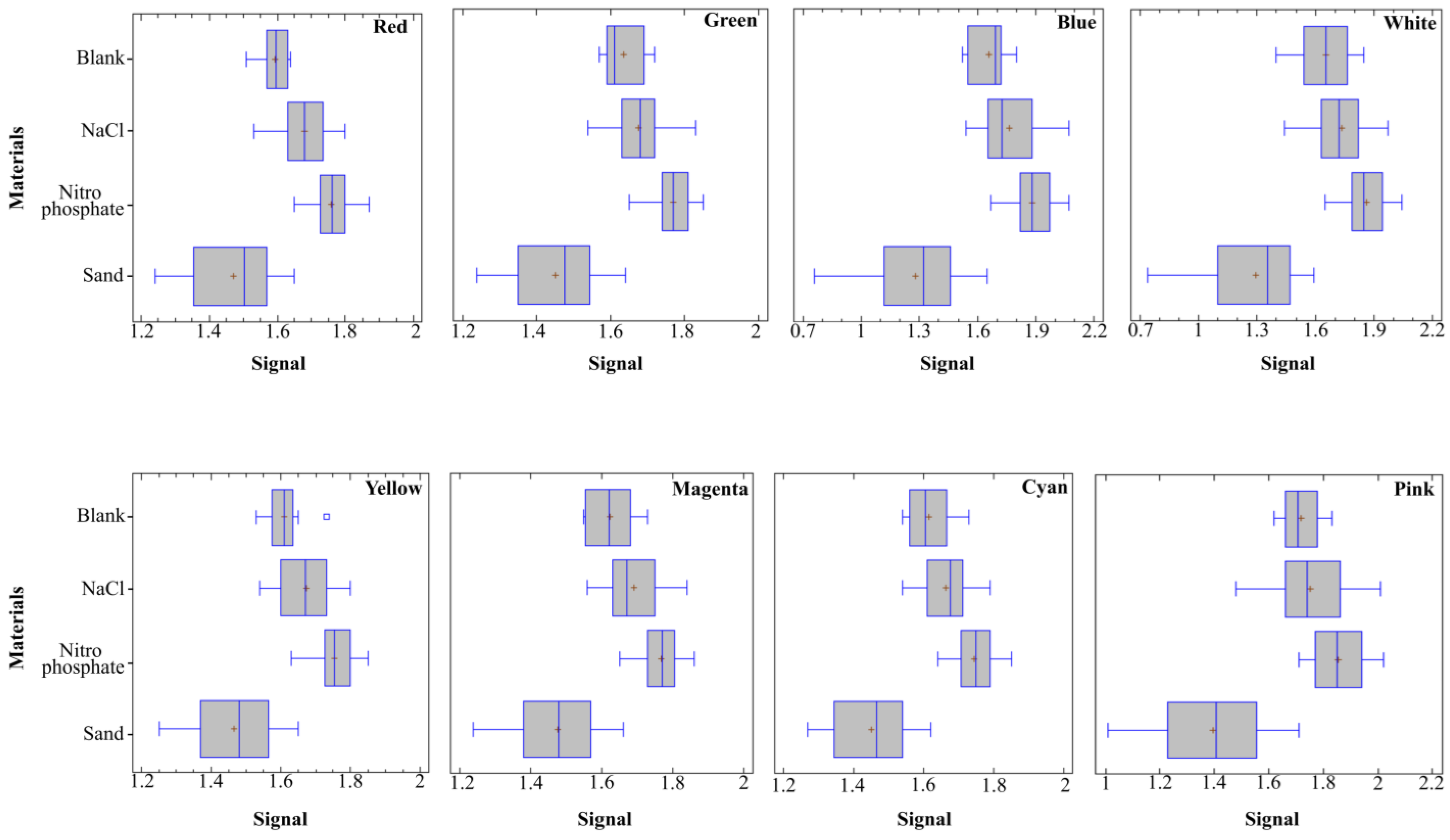
5.1. General Analyses
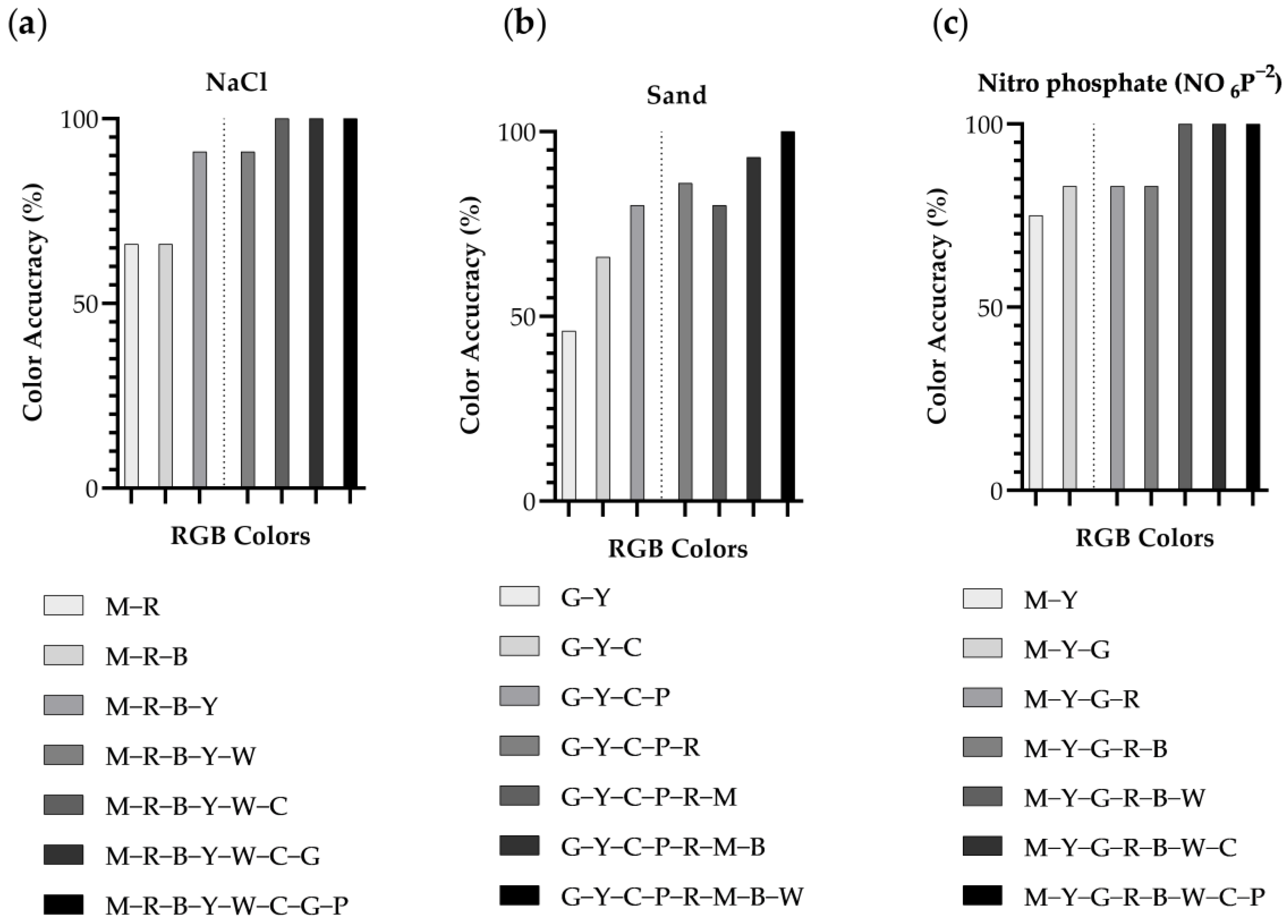
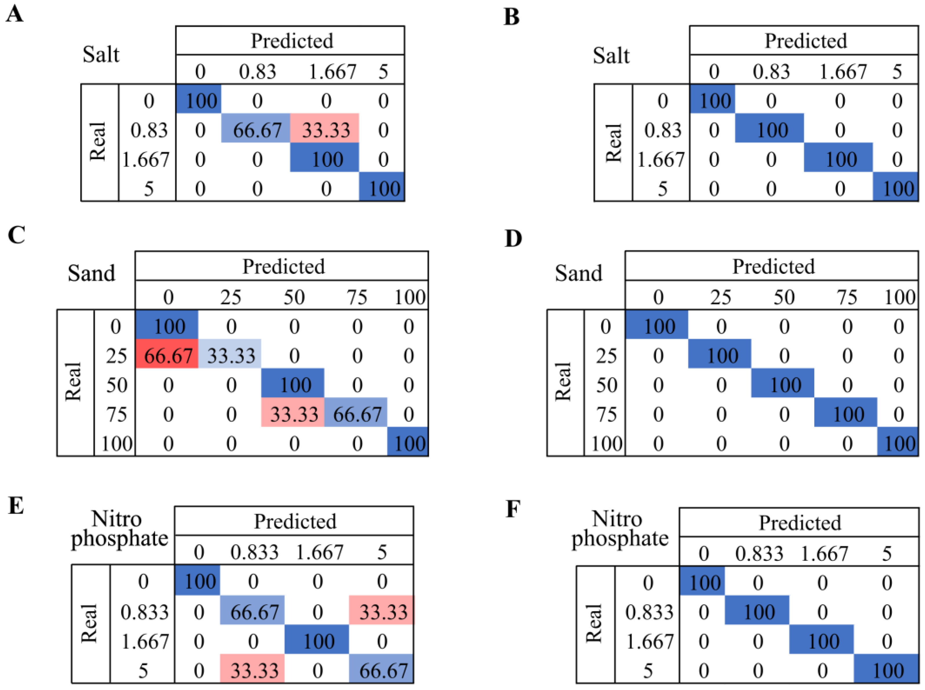
5.2. Classification of Subtances
6. Discussion
6.1. General Findings
6.1.1. Soil Texture Recognition
6.1.2. Salinity and Fertilizer Quantification

| Year | Data Type | Processing Technique | Parameter | Levels Min/ Max | No. of Classes | No. of Samples | Replicas | Type of Sample | Acc. | Ref. |
|---|---|---|---|---|---|---|---|---|---|---|
| 2019 | Images | PLSR | SSC (%) | 0–0.5 | - | 49 | - | Natural | - | [9] |
| 2020 | Images | PLSR or RF | SSC (%) | 0.08–5.4 | - | 93 | - | Natural | - | [43] |
| 2023 | Image pXRF, VIS, and NIR | CNN + RF+ SVM + GRU | SSC (%) | 5 | 240 | - | Natural | - | [35] | |
| 2022 | NIR–Vis | PLSR, RF | EC (mS/cm) | 0–10 | - | 231 | - | Natural | - | [44] |
| 2019 | NIR–Vis | Multiple | SSC (%) | 0.29–29.1 | - | 60 | 5 | Natural | - | [45] |
| 2024 | VIS data of LDR | DA | SSC (%) | 0.83–5 | 5 | 15 | 3 | Artificial | 100% | Proposal |
| 2023 | Soil sensors | CatBoost | Nutrients | - | - | - | - | Dataset | 97% | [30] |
| 2018 | Color sensors | NB | Fertility | - | 3 | 10 | - | Artificial | 80% | [47] |
| 2021 | UV–Vis | RF, SVM, ANN, NB | Nutrients (%) | 0–4 | 5 | 58 | - | Natural | 100% | [46] |
| 2024 | VIS data of LDR | DA | Nitro phosphate (%) | 0.83–5 | 5 | 15 | 3 | Artificial | 100% | Proposal |
6.1.3. Main Advantages of the Proposed Sensor
6.2. Limitations of Presented Results and Possible Future Solutions
7. Conclusions
Author Contributions
Funding
Institutional Review Board Statement
Informed Consent Statement
Data Availability Statement
Acknowledgments
Conflicts of Interest
References
- Trivedi, A.; Nandeha, N.; Mishra, S. Dryland agriculture and farming technology: Problems and Solutions. In Climate Resilient Smart Agriculture: Approaches & Techniques; Vital Biotech: Kota, India, 2022; pp. 35–51. [Google Scholar]
- Kumar, N.; Upadhyay, G.; Choudhary, S.; Patel, B.; Naresh; Chhokar, R.; Gill, S. Resource conserving mechanization technologies for dryland agriculture. In Enhancing Resilience of Dryland Agriculture under Changing Climate: Interdisciplinary and Convergence Approaches; Springer: Berlin/Heidelberg, Germany, 2023; pp. 657–688. [Google Scholar]
- Nijbroek, R.; Piikki, K.; Söderström, M.; Kempen, B.; Turner, K.G.; Hengari, S.; Mutua, J. Soil organic carbon baselines for land degradation neutrality: Map accuracy and cost tradeoffs with respect to complexity in Otjozondjupa, Namibia. Sustainability 2018, 10, 1610. [Google Scholar] [CrossRef]
- Pacheco, F.A.L.; Fernandes, L.F.S.; Junior, R.F.V.; Valera, C.A.; Pissarra, T.C.T. Land degradation: Multiple environmental consequences and routes to neutrality. Curr. Opin. Environ. Sci. Health 2018, 5, 79–86. [Google Scholar] [CrossRef]
- Maestre, F.T.; Benito, B.M.; Berdugo, M.; Concostrina-Zubiri, L.; Delgado-Baquerizo, M.; Eldridge, D.J.; Guirado, E.; Gross, N.; Kéfi, S.; Le Bagousse-Pinguet, Y. Biogeography of global drylands. New Phytol. 2021, 231, 540–558. [Google Scholar] [CrossRef] [PubMed]
- Ahmad, A.; Blasco, B.; Martos, V. Combating salinity through natural plant extracts based biostimulants: A review. Front. Plant Sci. 2022, 13, 862034. [Google Scholar] [CrossRef]
- Chimwamurombe, P.M.; Mataranyika, P.N. Factors influencing dryland agricultural productivity. J. Arid Environ. 2021, 189, 104489. [Google Scholar] [CrossRef]
- Rengasamy, P.; de Lacerda, C.F.; Gheyi, H.R. Salinity, sodicity and alkalinity. In Subsoil Constraints for Crop Production; Springer: Berlin/Heidelberg, Germany, 2022; pp. 83–107. [Google Scholar]
- Ngo, T.T.T.; Nguyen, H.Q.; Gorman, T.; Ngo Xuan, Q.; Ngo, P.L.T.; Vanreusel, A. Impacts of a saline water control project on aquaculture livelihoods in the Vietnamese Mekong Delta. J. Agribus. Dev. Emerg. Econ. 2023, 13, 418–436. [Google Scholar] [CrossRef]
- Corwin, D.L. Climate change impacts on soil salinity in agricultural areas. Eur. J. Soil Sci. 2021, 72, 842–862. [Google Scholar] [CrossRef]
- Chen, H.; Tian, Y.; Cai, Y.; Liu, Q.; Ma, J.; Wei, Y.; Yang, A. A 50-year systemic review of bioavailability application in Soil environmental criteria and risk assessment. Environ. Pollut. 2023, 335, 122272. [Google Scholar] [CrossRef]
- Nwaozuzu, C.; Nwosu, U.; Chikwendu, C. Geotechnical Characterization and Erosion Risk Assessment of Soils: A Case Study of Gomwalk Bridge, Federal University of Technology, Owerri, Southeastern Nigeria. Int. J. Adv. Acad. Res. 2023, 9, 113–137. [Google Scholar]
- Somma, R.; Spoto, S.E.; Raffaele, M.; Salmeri, F. Measuring color techniques for forensic comparative analyses of geological evidence. Atti Della Accad. Peloritana Dei Pericolanti-Cl. Di Sci. Fis. Mat. E Nat. 2023, 101, 14. [Google Scholar]
- Belenguer-Plomer, M.A.; Tanase, M.A.; Fernandez-Carrillo, A.; Chuvieco, E. Burned area detection and mapping using Sentinel-1 backscatter coefficient and thermal anomalies. Remote Sens. Environ. 2019, 233, 111345. [Google Scholar] [CrossRef]
- Nzuza, P.; Ramoelo, A.; Odindi, J.; Kahinda, J.M.; Madonsela, S. Predicting land degradation using Sentinel-2 and environmental variables in the Lepellane catchment of the Greater Sekhukhune District, South Africa. Phys. Chem. Earth Parts A/B/C 2021, 124, 102931. [Google Scholar] [CrossRef]
- García, L.; Parra, L.; Jimenez, J.M.; Lloret, J.; Lorenz, P. IoT-based smart irrigation systems: An overview on the recent trends on sensors and IoT systems for irrigation in precision agriculture. Sensors 2020, 20, 1042. [Google Scholar] [CrossRef]
- Cherubin, M.R.; Karlen, D.L.; Cerri, C.E.; Franco, A.L.; Tormena, C.A.; Davies, C.A.; Cerri, C.C. Soil quality indexing strategies for evaluating sugarcane expansion in Brazil. PLoS ONE 2016, 11, e0150860. [Google Scholar] [CrossRef]
- Ghoniemy, T.M.; Hammad, M.M.; Amein, A.; Mahmoud, T.A. Multi-stage guided-filter for SAR and optical satellites images fusion using Curvelet and Gram Schmidt transforms for maritime surveillance. Int. J. Image Data Fusion 2023, 14, 38–57. [Google Scholar] [CrossRef]
- Kulkarni, S.C.; Rege, P.P. Pixel level fusion techniques for SAR and optical images: A review. Inf. Fusion 2020, 59, 13–29. [Google Scholar] [CrossRef]
- Zhang, R.; Tang, X.; You, S.; Duan, K.; Xiang, H.; Luo, H. A novel feature-level fusion framework using optical and SAR remote sensing images for land use/land cover (LULC) classification in cloudy mountainous area. Appl. Sci. 2020, 10, 2928. [Google Scholar] [CrossRef]
- Pande, C.B.; Moharir, K.N. Application of hyperspectral remote sensing role in precision farming and sustainable agriculture under climate change: A review. In Climate Change Impacts on Natural Resources, Ecosystems and Agricultural Systems; Springer: Berlin/Heidelberg, Germany, 2023; pp. 503–520. [Google Scholar]
- Padmapriya, J.; Sasilatha, T. Deep learning based multi-labelled soil classification and empirical estimation toward sustainable agriculture. Eng. Appl. Artif. Intell. 2023, 119, 105690. [Google Scholar]
- de Carvalho Oliveira, G.; Machado, C.C.S.; Inácio, D.K.; da Silveira Petruci, J.F.; Silva, S.G. RGB color sensor for colorimetric determinations: Evaluation and quantitative analysis of colored liquid samples. Talanta 2022, 241, 123244. [Google Scholar] [CrossRef] [PubMed]
- de Oliveira Morais, P.A.; de Souza, D.M.; de Melo Carvalho, M.T.; Madari, B.E.; de Oliveira, A.E. Predicting soil texture using image analysis. Microchem. J. 2019, 146, 455–463. [Google Scholar] [CrossRef]
- Diaz, F.J.; Ahmad, A.; Viciano-Tudela, S.; Parra, L.; Sendra, S.; Lloret, J. Development of a Low-Cost Sensor to Optimise the Use of Fertilisers in Irrigation Systems. In Proceedings of the ICNS 2023: The Nineteenth International Conference on Networking and Services, Barcelona, Spain, 13–17 March 2023. [Google Scholar]
- Parra, L.; Viciano-Tudela, S.; Carrasco, D.; Sendra, S.; Lloret, J. Low-cost microcontroller-based multiparametric probe for coastal area monitoring. Sensors 2023, 23, 1871. [Google Scholar] [CrossRef]
- Pandiri, D.K.; Murugan, R.; Goel, T. Smart soil image classification system using lightweight convolutional neural network. Expert Syst. Appl. 2024, 238, 122185. [Google Scholar] [CrossRef]
- Han, P.; Dong, D.; Zhao, X.; Jiao, L.; Lang, Y. A smartphone-based soil color sensor: For soil type classification. Comput. Electron. Agric. 2016, 123, 232–241. [Google Scholar] [CrossRef]
- Al-Naji, A.; Fakhri, A.B.; Gharghan, S.K.; Chahl, J. Soil color analysis based on a RGB camera and an artificial neural network towards smart irrigation: A pilot study. Heliyon 2021, 7, e06078. [Google Scholar] [CrossRef] [PubMed]
- Islam, M.R.; Oliullah, K.; Kabir, M.M.; Alom, M.; Mridha, M. Machine learning enabled IoT system for soil nutrients monitoring and crop recommendation. J. Agric. Food Res. 2023, 14, 100880. [Google Scholar] [CrossRef]
- Tatli, S.; Mirzaee-Ghaleh, E.; Rabbani, H.; Karami, H.; Wilson, A.D. Rapid detection of urea fertilizer effects on voc emissions from cucumber fruits using a MOS E-Nose Sensor Array. Agronomy 2021, 12, 35. [Google Scholar] [CrossRef]
- Khodamoradi, F.; Mirzaee-Ghaleh, E.; Dalvand, M.J.; Sharifi, R. Classification of basil plant based on the level of consumed nitrogen fertilizer using an olfactory machine. Food Anal. Methods 2021, 14, 2617–2629. [Google Scholar] [CrossRef]
- Xu, L.; Zheng, C.; Wang, Z.; Nyongesah, M. A digital camera as an alternative tool for estimating soil salinity and soil surface roughness. Geoderma 2019, 341, 68–75. [Google Scholar] [CrossRef]
- Jahangeer, J.; Zhang, L.; Tang, Z. Assessing Salinity Dynamics of Saline Wetlands in Eastern Nebraska Using Continuous Data from Wireless Sensors. J. Hazard. Toxic Radioact. Waste 2024, 28, 04023035. [Google Scholar] [CrossRef]
- Gozukara, G.; Anagun, Y.; Isik, S.; Zhang, Y.; Hartemink, A.E. Predicting soil EC using spectroscopy and smartphone-based digital images. CATENA 2023, 231, 107319. [Google Scholar] [CrossRef]
- Lu, X.; Hui, W.; Si-yi, Q.; Jing-wen, L.; Li-juan, W. Coastal soil salinity estimation based digital images and color space conversion. Spectrosc. Spectr. Anal. 2021, 41, 2409–2414. [Google Scholar]
- Institute, N.G.; Gómez-Miguel, V. Soil Map of Spain. Available online: https://www.ign.es/web/catalogo-cartoteca/resources/html/030769.html (accessed on 11 December 2023).
- Munnaf, M.A.; Mouazen, A.M. Spectra transfer based learning for predicting and classifying soil texture with short-ranged Vis-NIRS sensor. Soil Tillage Res. 2023, 225, 105545. [Google Scholar] [CrossRef]
- Andrade, R.; Mancini, M.; dos Santos Teixeira, A.F.; Silva, S.H.G.; Weindorf, D.C.; Chakraborty, S.; Guilherme, L.R.G.; Curi, N. Proximal sensor data fusion and auxiliary information for tropical soil property prediction: Soil texture. Geoderma 2022, 422, 115936. [Google Scholar] [CrossRef]
- Dhawale, N.M.; Adamchuk, V.I.; Prasher, S.O.; Viscarra Rossel, R.A. Evaluating the Precision and Accuracy of Proximal Soil vis–NIR Sensors for Estimating Soil Organic Matter and Texture. Soil Syst. 2021, 5, 48. [Google Scholar] [CrossRef]
- Lazaar, A.; Pradhan, B.; Naiji, Z.; Gourfi, A.; El Hammouti, K.; Andich, K.; Monir, A. The manifestation of VIS-NIRS spectroscopy data to predict and mapping soil texture in the Triffa plain (Morocco). Kuwait J. Sci. 2021, 48. [Google Scholar] [CrossRef]
- Mancini, M.; Andrade, R.; Silva, S.H.G.; Rafael, R.B.A.; Mukhopadhyay, S.; Li, B.; Chakraborty, S.; Guilherme, L.R.G.; Acree, A.; Weindorf, D.C.; et al. Multinational prediction of soil organic carbon and texture via proximal sensors. Soil Sci. Soc. Am. J. 2023, 88, 8–26. [Google Scholar] [CrossRef]
- Xu, L.; Rossel RA, V.; Lee, J.; Wang, Z.; Ma, H. A simple approach to estimate coastal soil salinity using digital camera images. Soil Res. 2020, 58, 737–747. [Google Scholar] [CrossRef]
- Jia, P.; Zhang, J.; He, W.; Yuan, D.; Hu, Y.; Zamanian, K.; Jia, K.; Zhao, X. Inversion of Different Cultivated Soil Types’ Salinity Using Hyperspectral Data and Machine Learning. Remote Sens. 2022, 14, 5639. [Google Scholar] [CrossRef]
- Wang, S.; Chen, Y.; Wang, M.; Li, J. Performance comparison of machine learning algorithms for estimating the soil salinity of salt-affected soil using field spectral data. Remote Sens. 2019, 11, 2605. [Google Scholar] [CrossRef]
- Trontelj ml, J.; Chambers, O. Machine learning strategy for soil nutrients prediction using spectroscopic method. Sensors 2021, 21, 4208. [Google Scholar] [CrossRef]
- Agarwal, S.; Bhangale, N.; Dhanure, K.; Gavhane, S.; Chakkarwar, V.A.; Nagori, M.B. Application of colorimetry to determine soil fertility through naive bayes classification algorithm. In Proceedings of the 2018 9th International Conference on Computing, Communication and Networking Technologies (ICCCNT), Bengaluru, India, 10–12 July 2018; pp. 1–6. [Google Scholar]
- Viciano-Tudela, S.; Sendra, S.; Parra, L.; Jimenez, J.M.; Lloret, J. Proposal of a Gas Sensor-Based Device for Detecting Adulteration in Essential Oil of Cistus ladanifer. Sustainability 2023, 15, 3357. [Google Scholar] [CrossRef]


| Study | Year | Main Findings | Methodology | Limitations/Challenges |
|---|---|---|---|---|
| [28] | 2016 | Over 90% accuracy in DA for soil classification based on smartphone images. | Conversion of soil images to RGB signal, DA. | Challenges in varying light conditions and the drying of soil samples as a preliminary step. |
| [24] | 2019 | 100% match in soil texture prediction using multivariate image analysis. | Multivariate image analysis of soil samples. | Limited validation datasets, applicability to soils with higher silt contents not tested. |
| [29] | 2021 | Successful decision making about soil irrigation using RGB image analysis using ANN. | RGB image analysis, feed-forward backpropagation neural network. | Need for validation across different soil types and conditions, consideration of environmental factors for real-world deployment. |
| [27] | 2024 | 97.2% accuracy in classifying sand, clay, loam, loamy sand, and sandy loam using a camera. | RGB extraction, V extraction from HSV bins, adaptive histogram, Light-SoilNet CNN. | Requires a diverse dataset, challenges in real-time implementation in agriculture. |
| [31] | 2021 | 98.67% accuracy in VOC emissions analysis based on urea–nitrogen fertilizer rates. | MOS electronic nose, quadratic DA. | Data acquisition susceptible to environmental influences. |
| [32] | 2021 | 95–97.78% accuracy in classifying basil plants based on urea fertilizer. | LDA, QDA, various analytical approaches. | Only detects the nitrogen volatile compounds in the plant. |
| [25] | 2023 | 100% accuracy in predicting fertilizer concentration using an ANN model. | Two-Coil Systems sensor, ANN. | Lack of simplicity, susceptibility to diverse environmental influences. |
| [30] | 2023 | 97.5% accuracy in predicting organic matter, potassium oxide, and phosphorus pentoxide in soil using CatBoost. | Multiple linear regression, SVM, RF, CatBoost classifier. | Constraints associated with data accessibility, susceptibility to errors, system intricacy, cost considerations, and maintenance. |
| [33] | 2019 | R2 of 0.90 for soil salt content and 0.71 for soil surface roughness prediction. | Digital camera, four-color component prediction model. | Limited generalizability to different environments, dependency on environmental conditions, and challenges in scaling up. |
| [36] | 2021 | Overall accuracy of R2 = 0.75 based on digital photographs for soil salinity | Digital photographs, correlation analysis, RF. | Generalizability challenges, concerns about model interpretation, data privacy, and security. |
| [35] | 2023 | R2 of 0.93 for predicting EC using Combined Vis–NIR and pXRF spectra. | Smartphone-based color coordinates, Vis–NIR, pXRF spectra, RF. | Challenges in generalizability, reliance on correlated parameters, sensitivity to temporal variability. |
| [34] | 2024 | Identified topsoil degradation by increasing salinity. | HYDRO 21 and TEROS 12 sensors, Pearson correlation. | Point-level salinity measurement and limited duration. |
| Sample ID | Test | Concentration (%)/(Numbers) | Added Substance (g) | |||
|---|---|---|---|---|---|---|
| Soil | NaCl | Sand | Nitro Phosphate (NO6P−2) | |||
| 1 | Blank | 0 | 3 | - | - | - |
| 2 | Salt | 0.83 | 3 | 0.025 | - | - |
| 3 | 1.67 | 3 | 0.05 | - | - | |
| 4 | 3.33 | 3 | 0.1 | - | - | |
| 5 | 5 | 3 | 0.15 | - | - | |
| 6 | Sand | 25 | 2.25 | - | 0.75 | - |
| 7 | 50 | 1.5 | - | 1.5 | - | |
| 8 | 75 | 0.75 | - | 2.25 | - | |
| 9 | 100 | 0 | - | 3 | - | |
| 10 | Nitro phosphate | 0.83 | 3 | - | - | 0.025 |
| 11 | 1.67 | 3 | - | - | 0.05 | |
| 12 | 3.33 | 3 | - | - | 0.1 | |
| 13 | 5 | 3 | - | - | 0.15 | |
| Light | Blank | NaCl | Sand | Nitro Phosphate (NO6P−2) | ||||
|---|---|---|---|---|---|---|---|---|
| Original | Modified | Original | Modified | Original | Modified | Original | Modified | |
| Red | 497.67 | 1.59 | 504 | 1.69 | 488.67 | 1.52 | 511 | 1.77 |
| Green | 510.33 | 1.61 | 504.67 | 1.64 | 494.67 | 1.51 | 516.33 | 1.78 |
| Blue | 555.33 | 1.73 | 556.33 | 1.72 | 541 | 1.40 | 567.67 | 1.96 |
| Light | Percentage of Concentration | p-Value | ||||
|---|---|---|---|---|---|---|
| 0 | 0.83 | 1.67 | 3.33 | 5 | ||
| Red | 1.59 a | 1.66 ab | 1.69 b | 1.67 b | 1.71 b | 0.013 |
| Green | 1.64 a | 1.66 a | 1.63 a | 1.67 a | 1.74 b | 0.011 |
| Blue | 1.66 a | 1.70 a | 1.72 a | 1.75 ab | 1.87 b | 0.014 |
| White | 1.65 a | 1.69 ab | 1.71 ab | 1.72 ab | 1.82 b | 0.147 |
| Yellow | 1.61 a | 1.66 ab | 1.64 ab | 1.68 b | 1.71 b | 0.052 |
| Magenta | 1.62 a | 1.66 ab | 1.66 ab | 1.69 bc | 1.75 c | 0.008 |
| Cyan | 1.62 a | 1.65 a | 1.62 a | 1.66 a | 1.72 b | 0.005 |
| Pink | 1.72 a | 1.71 a | 1.73 ab | 1.72 a | 1.84 b | 0.147 |
| Light | Percentage of Concentration | p-Value | ||||
|---|---|---|---|---|---|---|
| 0 | 25 | 50 | 75 | 100 | ||
| Red | 1.59 a | 1.47 bc | 1.49 b | 1.54 ab | 1.38 c | 0.001 |
| Green | 1.64 a | 1.47 b | 1.46 b | 1.51 b | 1.37 c | 0.0001 |
| Blue | 1.66 a | 1.28 bc | 1.27 bc | 1.39 b | 1.17 c | 0.0003 |
| White | 1.65 a | 1.27 bc | 1.34 bc | 1.40 b | 1.16 c | 0.0003 |
| Yellow | 1.61 a | 1.48 b | 1.51 b | 1.52 b | 1.34 c | 0.0001 |
| Magenta | 1.62 a | 1.49 b | 1.50 b | 1.53 ab | 1.38 c | 0.0002 |
| Cyan | 1.62 a | 1.48 b | 1.46 b | 1.50 b | 1.36 c | 0.0001 |
| Pink | 1.72 a | 1.42 b | 1.43 b | 1.43 b | 1.30 b | 0.0003 |
| Light | Percentage of Concentration | p-Value | ||||
|---|---|---|---|---|---|---|
| 0 | 0.83 | 1.67 | 3.33 | 5 | ||
| Red | 1.59 a | 1.77 c | 1.71 b | 1.76 c | 1.80 c | 0.0001 |
| Green | 1.64 a | 1.78 c | 1.72 b | 1.77 c | 1.80 c | 0.0001 |
| Blue | 1.66 a | 1.90 c | 1.89 b | 1.92 c | 1.90 c | 0.0001 |
| White | 1.65 a | 1.88 c | 1.76 b | 1.88 c | 1.91 c | 0.0001 |
| Yellow | 1.61 a | 1.75 bc | 1.72 b | 1.77 bc | 1.79 c | 0.0001 |
| Magenta | 1.62 a | 1.76 b | 1.74 b | 1.78 b | 1.78 b | 0.0001 |
| Cyan | 1.62 a | 1.74 bc | 1.70 b | 1.78 c | 1.75 bc | 0.0001 |
| Pink | 1.72 a | 1.8 9c | 1.79 ab | 1.88 c | 1.85 bc | 0.0001 |
| Year | Data Type | Processing Technique | No. of Classes | No. of Samples | Replicas | Type of Sample | Acc. | Ref. |
|---|---|---|---|---|---|---|---|---|
| 2024 | Image | CNN | 5 | 392 | - | Natural | 97.2% | [27] |
| 2019 | Image | MIA | 6 | 63 | - | Natural | 100% | [24] |
| 2022 | pXRF, VIS, and NIR data | RF | 4 | 464 | - | Natural | 97% | [39] |
| 2023 | VIS and NIR data | PLSR | - | 94 | - | Natural | 70–90% | [38] |
| 2021 | VIS and NIR data | PLSR | - | 19 | - | Natural | - | [40] |
| 2023 | pXRF, VIS, and NIR data | RFE + RF | - | 1545 | 3 | Natural | - | [42] |
| 2021 | VIS and NIR | PLSR | - | 100 | - | Natural | - | [41] |
| 2024 | VIS data of LDR | DA | 5 | 15 | 3 | Artificial | 100% | Proposal |
Disclaimer/Publisher’s Note: The statements, opinions and data contained in all publications are solely those of the individual author(s) and contributor(s) and not of MDPI and/or the editor(s). MDPI and/or the editor(s) disclaim responsibility for any injury to people or property resulting from any ideas, methods, instructions or products referred to in the content. |
© 2024 by the authors. Licensee MDPI, Basel, Switzerland. This article is an open access article distributed under the terms and conditions of the Creative Commons Attribution (CC BY) license (https://creativecommons.org/licenses/by/4.0/).
Share and Cite
Diaz, F.J.; Ahmad, A.; Parra, L.; Sendra, S.; Lloret, J. Low-Cost Optical Sensors for Soil Composition Monitoring. Sensors 2024, 24, 1140. https://doi.org/10.3390/s24041140
Diaz FJ, Ahmad A, Parra L, Sendra S, Lloret J. Low-Cost Optical Sensors for Soil Composition Monitoring. Sensors. 2024; 24(4):1140. https://doi.org/10.3390/s24041140
Chicago/Turabian StyleDiaz, Francisco Javier, Ali Ahmad, Lorena Parra, Sandra Sendra, and Jaime Lloret. 2024. "Low-Cost Optical Sensors for Soil Composition Monitoring" Sensors 24, no. 4: 1140. https://doi.org/10.3390/s24041140
APA StyleDiaz, F. J., Ahmad, A., Parra, L., Sendra, S., & Lloret, J. (2024). Low-Cost Optical Sensors for Soil Composition Monitoring. Sensors, 24(4), 1140. https://doi.org/10.3390/s24041140