
A 0.05 m Change in Inertial Measurement Unit Placement Alters Time and Frequency Domain Metrics during Running

 ,
,  ,
,  and
and
Abstract
1. Introduction
2. Methods
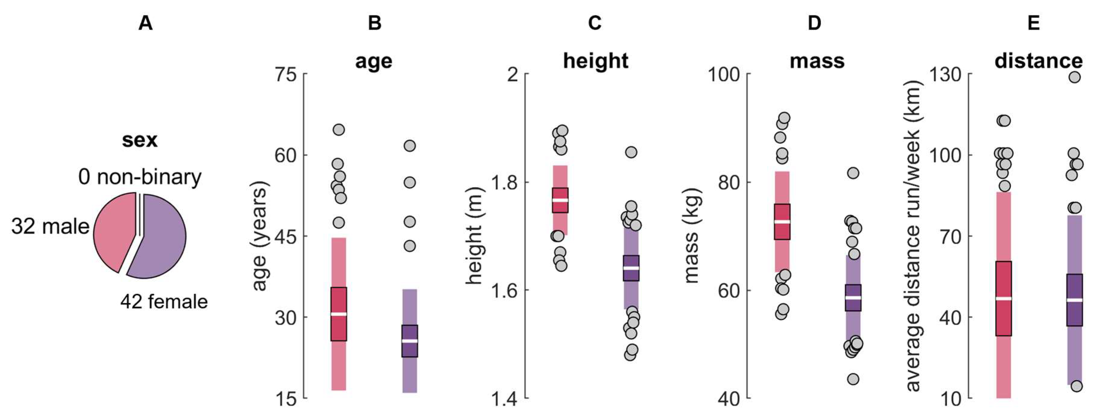
2.1. Participants
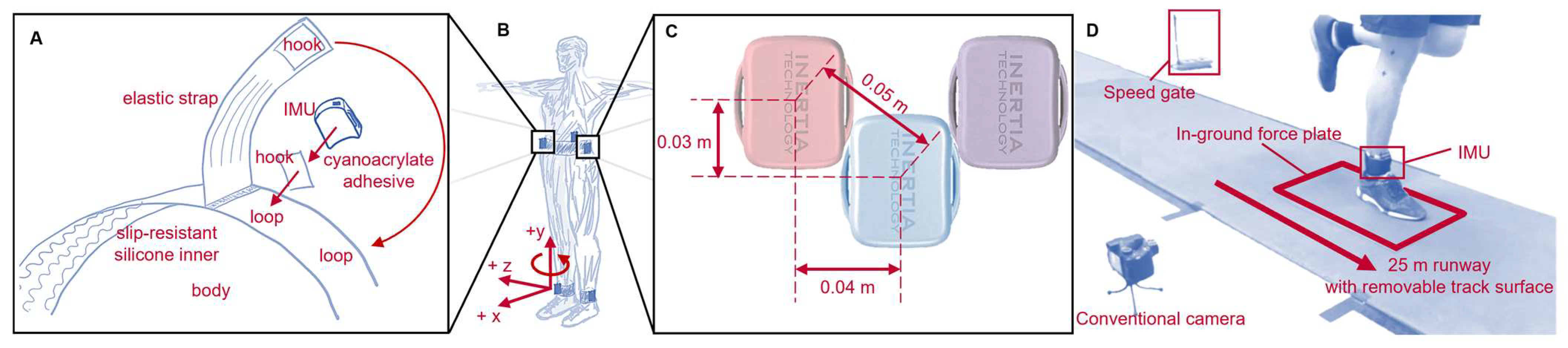
2.2. IMU Placement
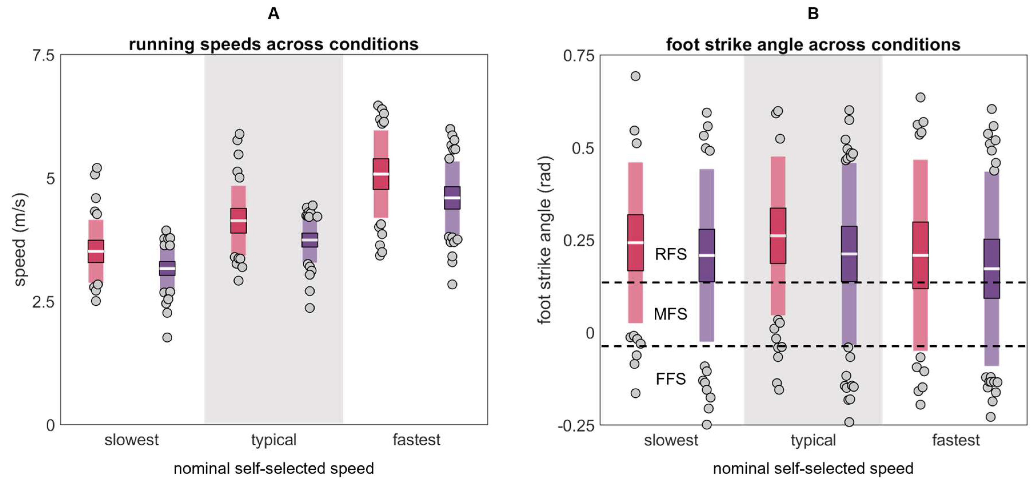
2.3. Protocol
2.4. Processing
2.5. Analysis
3. Results
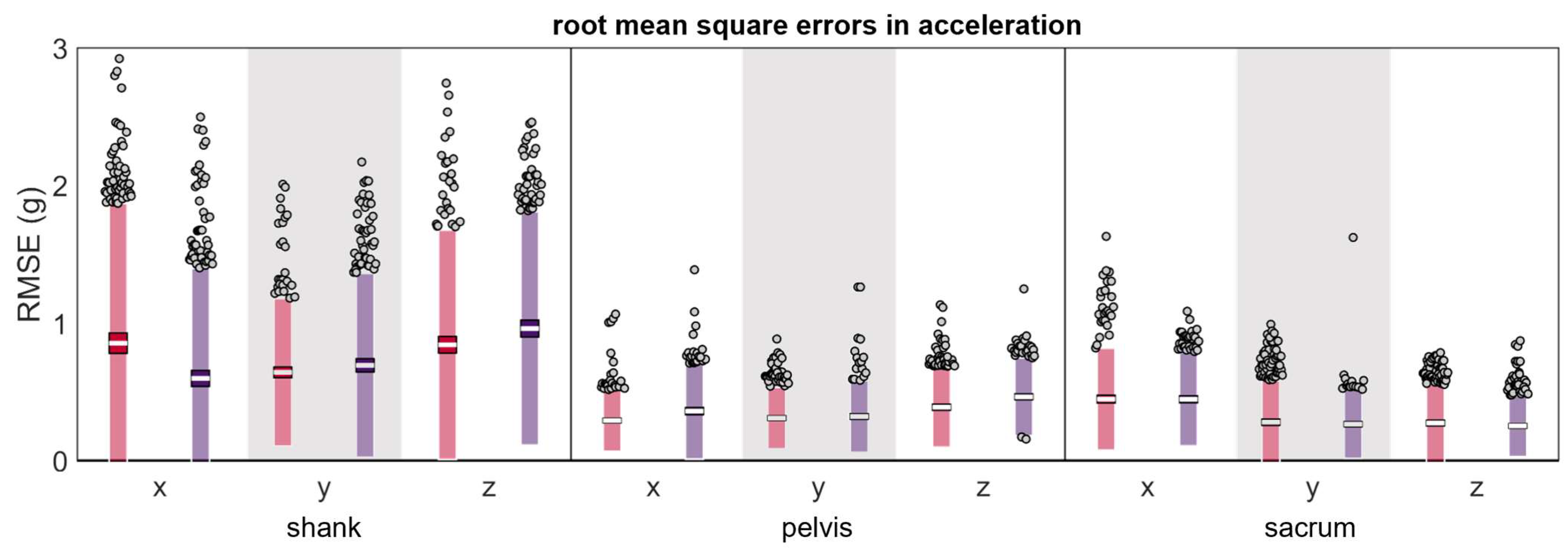
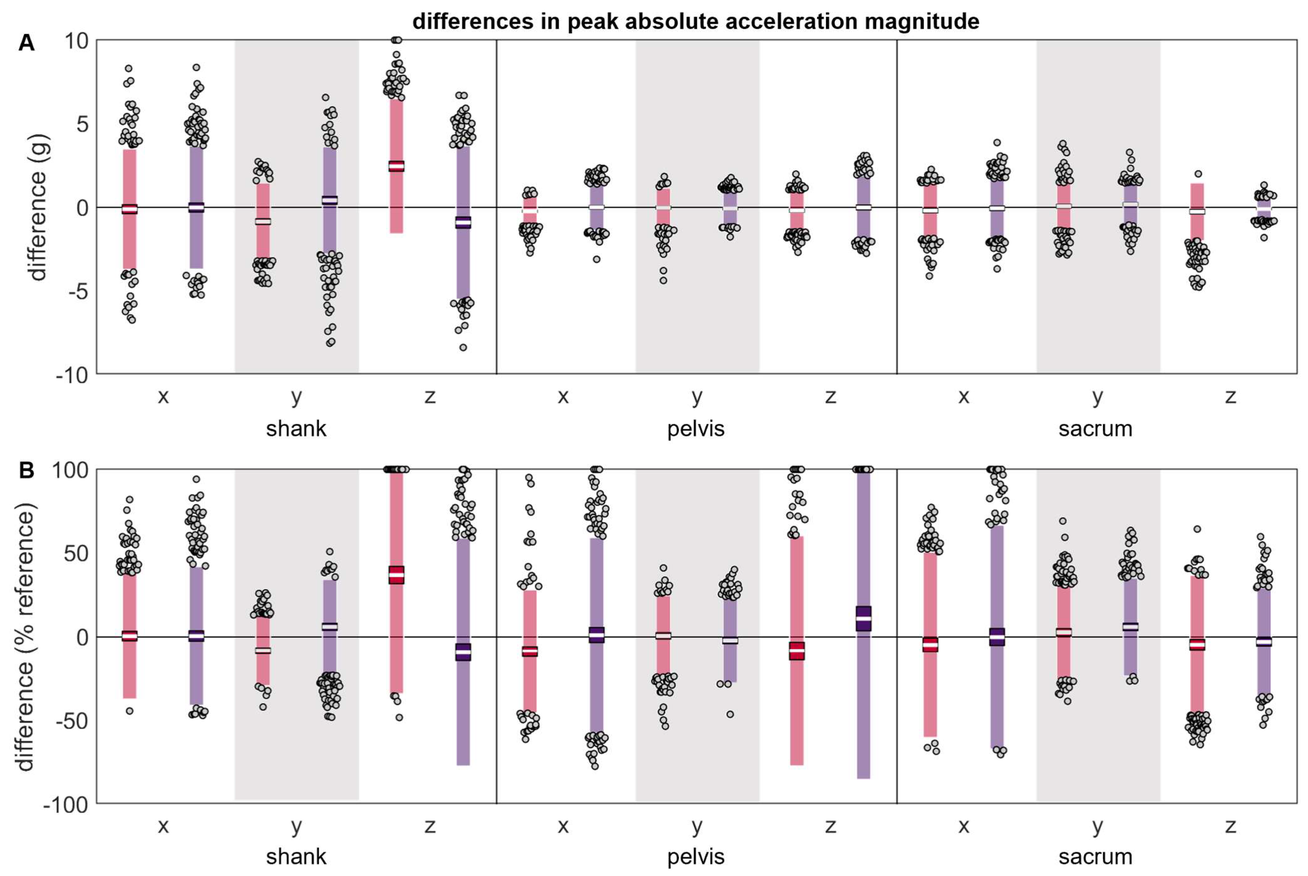
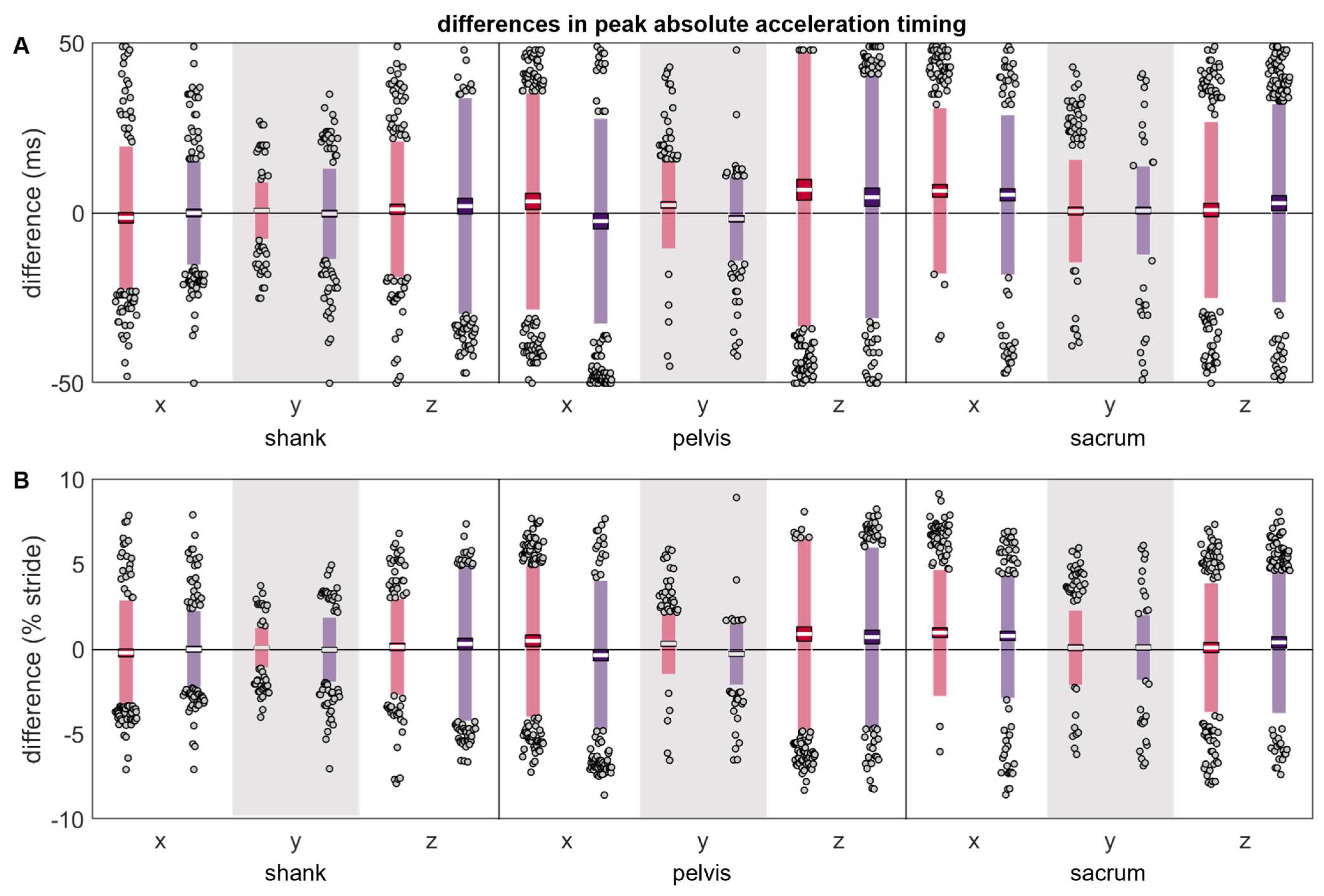
3.1. Acceleration
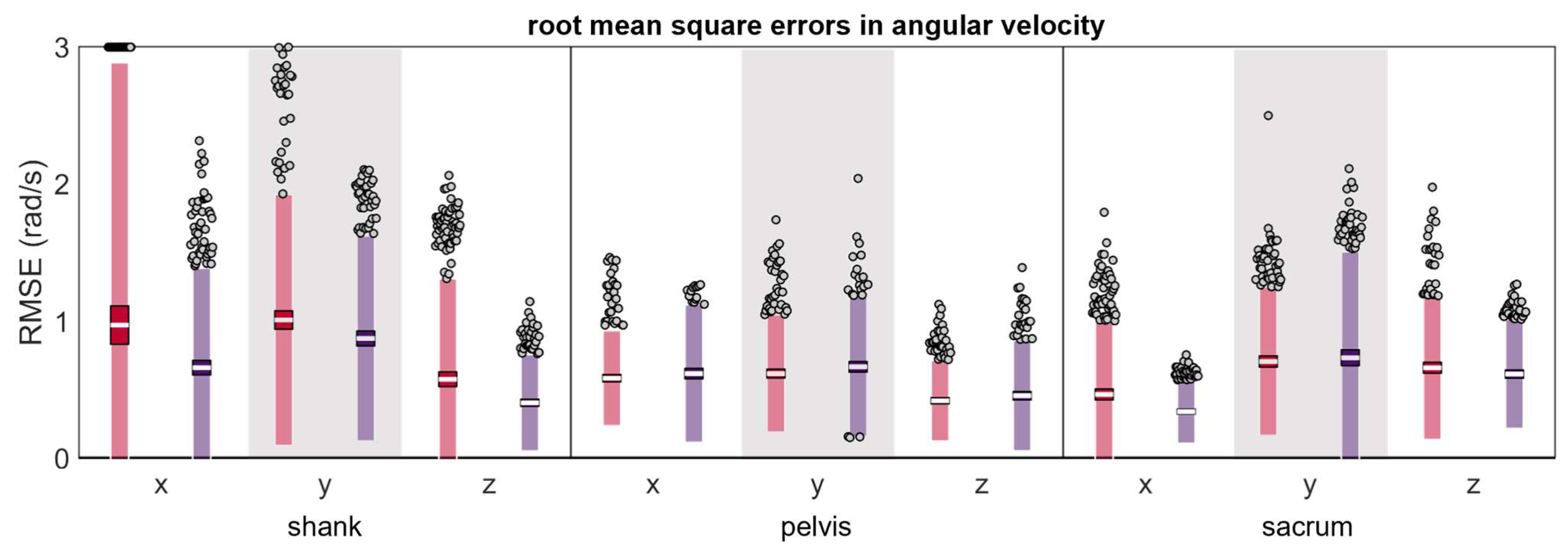
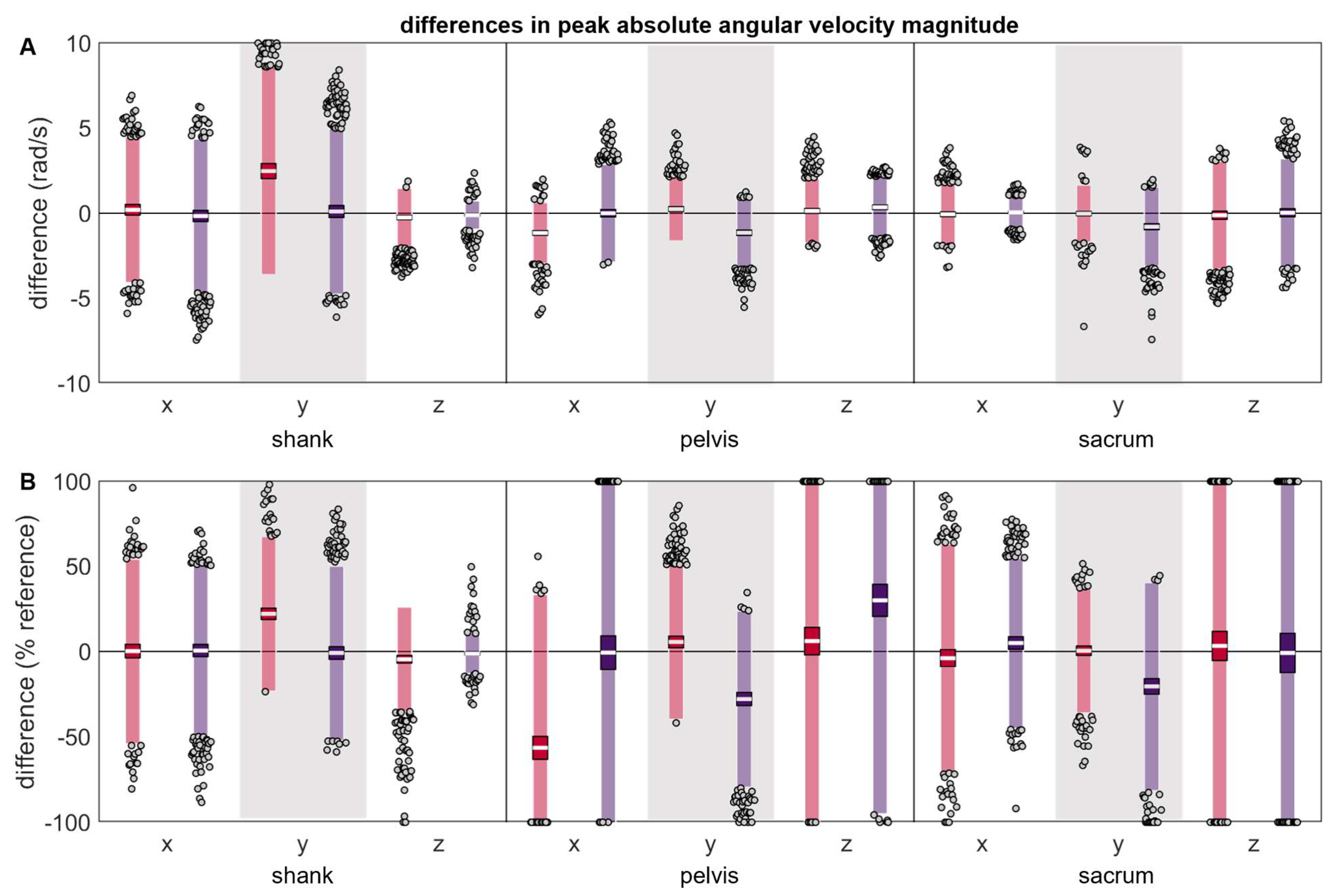
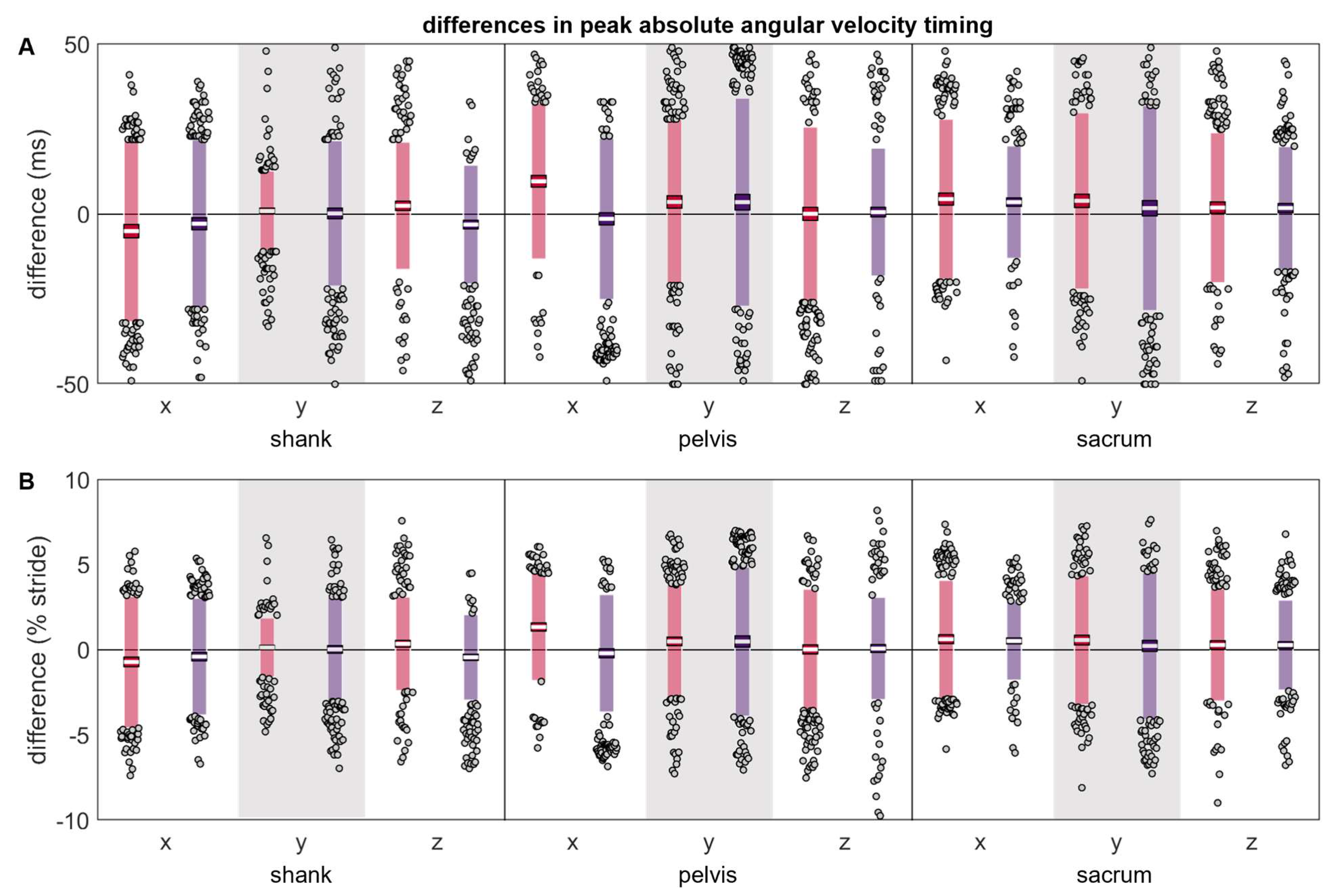
3.2. Angular Velocity
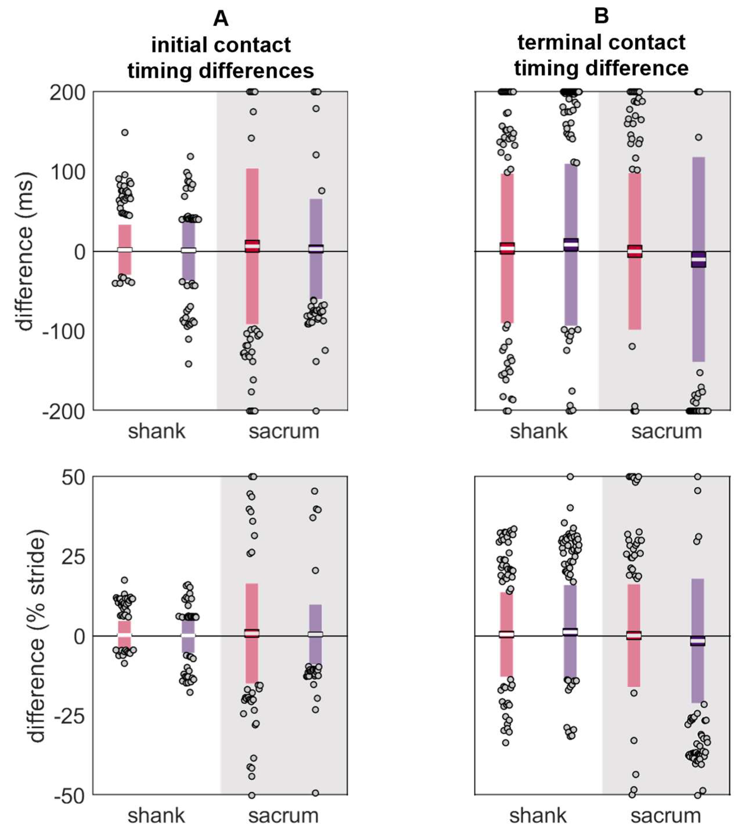
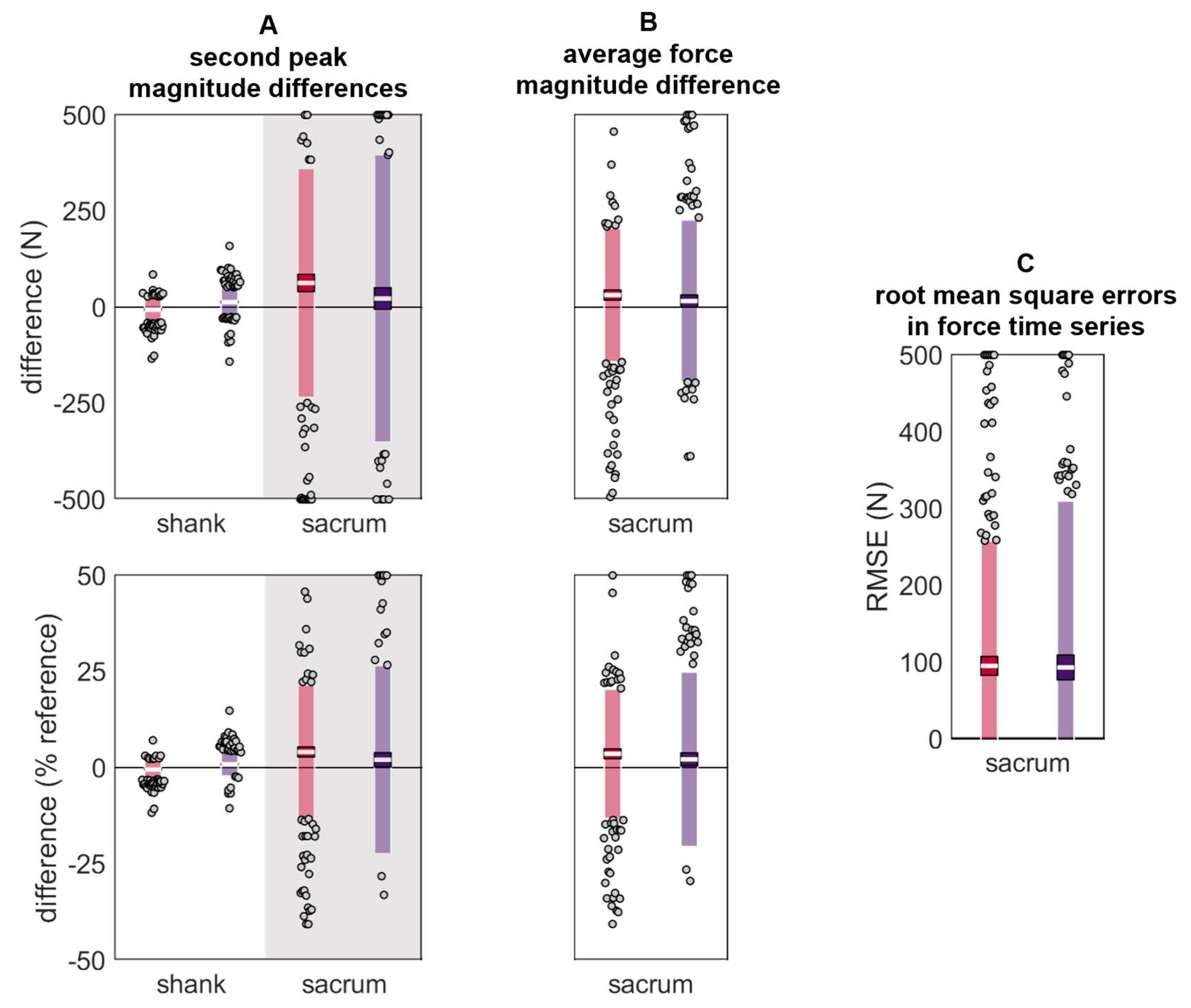
3.3. Estimated Outcome Variables
4. Discussion
5. Conclusions
Supplementary Materials
Author Contributions
Funding
Institutional Review Board Statement
Informed Consent Statement
Data Availability Statement
Conflicts of Interest
References
- Fong, D.T.P.; Chan, Y.Y. The use of wearable inertial motion sensors in human lower limb biomechanics studies: A systematic review. Sensors 2010, 10, 11556–11565. [Google Scholar] [CrossRef]
- Thiel, D.; Shepherd, J.; Espinosa, H.; Kenny, M.; Fischer, K.; Worsey, M.; Matsuo, A.; Wada, T. Predicting Ground Reaction Forces in Sprint Running Using a Shank Mounted Inertial Measurement Unit. Proceedings 2018, 2, 199. [Google Scholar]
- Raper, D.; Witchalls, J.; Phillips, E.; Drew, M. Use of a tibial accelerometer to measure ground reaction force in running: A reliability and validity comparison with force plates. J. Sci. Med. Sport 2018, 21, 84–88. [Google Scholar] [CrossRef] [PubMed]
- Owings, T.; Grabiner, M. Measuring step kinematic variability on an instrumented treadmill: How many steps are enough? J. Biomech. 2003, 36, 1215–1218. [Google Scholar] [CrossRef] [PubMed]
- Karatsidis, A.; Schepers, M. Estimation of Ground Reaction Forces and Moments During Gait Using Only Inertial Motion Capture. Sensors 2016, 17, 75. [Google Scholar] [CrossRef] [PubMed]
- Guo, Y.; Storm, F.; Zhao, Y.; Billings, S.; Pavic, A.; Mazza, C.; Guo, L. A New Proxy Measurement Algorithm with Application to the Estimation of Vertical Ground Reaction Forces Using Wearable Sensors. Sensors 2017, 17, 2181. [Google Scholar] [CrossRef] [PubMed]
- Chambon, N.; Delattre, N.; Gueguen, N.; Berton, E.; Rao, G. Shoe drop has opposite influence on running pattern when running overground or on a treadmill. Eur. J. Appl. Physiol. 2015, 115, 911–918. [Google Scholar] [CrossRef]
- Johnson, C.; Outerleys, J.; Jamison, S.; Tenforde, A.; Ruder, M.; Davis, I. Comparison of Tibial Shock during Treadmill and Real-World Running. Med. Sci. Sports Exerc. 2020, 52, 1557–1562. [Google Scholar] [CrossRef]
- Paquette, M.; Melcher, D. Impact of a Long Run on Injury-Related Biomechanics with Relation to Weekly Mileage in Trained Male Runners. J. Appl. Biomech. 2017, 33, 216–221. [Google Scholar] [CrossRef]
- van der Worp, H.; Vrielink, J.W.; Bredeweg, S.W. Do runners who suffer injuries have higher vertical ground reaction forces than those who remain injury free? A systematic review and meta-analysis. Br. J. Sports Med. 2016, 50, 450–457. [Google Scholar] [CrossRef]
- Willy, R.W. Innovations and pitfalls in the use of wearable devices in the prevention and rehabilitation of running related injuries. Phys. Ther. Sport 2018, 29, 26–33. [Google Scholar] [CrossRef] [PubMed]
- Running USA. 2017 National Runner Survey. 2017. Available online: https://www.runningusa.org/product-category/research/surveys-studies/ (accessed on 5 June 2019).
- Janssen, M.; Scheerder, J.; Thibaut, E.; Brombacher, A.; Vos, S. Who uses running apps and sport watches? Determinants and consumer profiles of event runners’ usage of running-related smartphone applications and smart watches. PLoS ONE 2017, 12, e0181167. [Google Scholar] [CrossRef] [PubMed]
- Pobiruchin, M.; Suleder, J.; Zowalla, R.; Wiesner, M.; Wilson, G.; Mauriello, M.; Cena, F. Accuracy and Adoption of Wearable Technology Used by Active Citizens: A Marathon Event Field Study. JMIR mHealth uHealth 2017, 5, e24. [Google Scholar] [CrossRef] [PubMed]
- Clermont, C.; Duffett-Leger, L.; Hettinga, B.; Ferber, R. Runners’ Perspectives on ‘Smart’ Wearable Technology and Its Use for Preventing Injury. Int. J. Hum. Comput. Interact. 2019, 36, 31–40. [Google Scholar] [CrossRef]
- Kiernan, D.; Dunn-Siino, K.; Hawkins, D. Unsupervised Gait Event Identification with a Single Wearable Accelerometer and/or Gyroscope: A Comparison of Methods across Running Speeds, Surfaces, and Foot Strike Patterns. Sensors 2023, 23, 5022. [Google Scholar] [CrossRef] [PubMed]
- Kiernan, D.; Ng, B.; Hawkins, D. Acceleration-Based Estimation of Vertical Ground Reaction Forces during Running: A Comparison of Methods across Running Speeds, Surfaces, and Foot Strike Patterns. Sensors 2023, 23, 8719. [Google Scholar] [CrossRef]
- Falbriard, M.; Soltani, A.; Aminian, K. Running Speed Estimation Using Shoe-Worn Inertial Sensors: Direct Integration, Linear, and Personalized Model. Front. Sports Act. Living 2021, 3, 585809. [Google Scholar] [CrossRef]
- Hernandez, V.; Dadkhah, D.; Babakeshizadeh, V.; Kulic, D. Lower body kinematics estimation from wearable sensors for walking and running: A deep learning approach. Gait Posture 2021, 83, 185–193. [Google Scholar] [CrossRef]
- Reenalda, J.; Maartens, E.; Buurke, J.; Gruber, A. Kinematics and shock attenuation during a prolonged run on the athletic track as measured with inertial magnetic measurement units. Gait Posture 2019, 68, 155–160. [Google Scholar] [CrossRef]
- Reenalda, J.; Maartens, E.; Homan, L.; Buurke, J. Continuous three dimensional analysis of running mechanics during a marathon by means of inertial Magn. measurement units to objectify changes in running mechanics. J. Biomech. 2016, 49, 3362–3367. [Google Scholar] [CrossRef]
- Ruder, M.; Jamison, S.; Tenforde, A.; Mulloy, F.; Davis, I. Relationship of Foot Strike Pattern and Landing Impacts during a Marathon. Med. Sci. Sports Exerc. 2019, 51, 2073–2079. [Google Scholar] [CrossRef] [PubMed]
- Melo, C.; Carpes, F.; Vieira, T.; Mendes, T.; de Paula, L.; Chagas, M.; Peixoto, G.; de Andrade, A.P. Correlation between running asymmetry, mechanical efficiency, and performance during a 10 km run. J. Biomech. 2020, 109, 109913. [Google Scholar] [CrossRef] [PubMed]
- Meyer, F.; Falbriard, M.; Mariani, B.; Aminian, K.; Millet, G. Continuous Analysis of Marathon Running Using Inertial Sensors: Hitting Two Walls? Int. J. Sports Med. 2021, 42, 1182–1190. [Google Scholar] [CrossRef] [PubMed]
- Kiernan, D.; Hawkins, D.; Manoukian, M.; McKallip, M.; Oelsner, L.; Caskey, C.; Coolbaugh, C. Accelerometer-based prediction of running injury in National Collegiate Athletic Association track athletes. J. Biomech. 2018, 73, 201–209. [Google Scholar] [CrossRef] [PubMed]
- Gruber, A.; McDonnell, J.; Davis, J.; Vollmar, J.; Harelak, J.; Paquette, M. Monitoring Gait Complexity as an Indicator for Running-Related Injury Risk in Collegiate Cross-Country Runners: A Proof-of-Concept Study. Front. Sport Act. Living 2021, 21, 630975. [Google Scholar] [CrossRef] [PubMed]
- Moran, D.; Evans, R.; Arbel, Y.; Luria, O.; Hadid, A.; Yanovich, R.; Milgrom, C.; Finestone, A. Physical and psychological stressors linked with stress fractures in recruit training. Scand. J. Med. Sci. Sports 2013, 23, 443–450. [Google Scholar] [CrossRef] [PubMed]
- Lempke, A.D.; Hart, J.; Hryvniak, D.; Rodu, J.; Hertel, J. Running-Related Injuries Captured Using Wearable Technology during a Cross-Country Season: A Preliminary Study. Transl. J. Am. Coll. Sports Med. 2023, 8, e000217. [Google Scholar]
- Wood, C.; Kipp, K. Use of Audio Biofeedback to Reduce Tibial Impact Accelerations During Running. J. Biomech. 2014, 47, 1739–1741. [Google Scholar] [CrossRef]
- Giraldo-Pedroza, A.; Lee, W.; Lam, W.; Coman, R.; Alici, G. Effects of Wearable Devices with Biofeedback on Biomechanical Performance of Running—A Systematic Review. Sensors 2020, 20, 6637. [Google Scholar] [CrossRef]
- Morris, J.; Goss, D.; Miller, E.; Davis, I. Using real-time biofeedback to alter running biomechanics: A randomized controlled trial. Transl. Sports Med. 2020, 3, 63–71. [Google Scholar] [CrossRef]
- Van Hooren, B.; Goudsmit, J.; Restrepo, J.; Vos, S. Real-time feedback by wearables in running: Current approaches, challenges and suggestions for improvements. J. Sports Sci. 2020, 38, 214–230. [Google Scholar] [CrossRef] [PubMed]
- Napier, C.; Esculier, J.; Hunt, M. Gait retraining: Out of the lab and onto the streets with the benefit of wearables. British J. Sports Med. 2017, 51, 1642–1643. [Google Scholar] [CrossRef] [PubMed]
- Tan, T.; Chiasson, D.; Hu, H.; Shull, P. Influence of IMU position and orientation placement errors on ground reaction force estimation. J. Biomech. 2019, 97, 109416. [Google Scholar] [CrossRef] [PubMed]
- Ruder, M.; Hunt, M.; Charlton, J.; Tse, C. Validity and reliability of gait metrics derived from researcher-placed and self-placed wearable inertial sensors. J. Biomech. 2022, 142, 111263. [Google Scholar] [CrossRef] [PubMed]
- Chen, S.; Brantley, J.; Kim, T.; Ridenour, S.; Lach, J. Characterizing and Minimizing Sources of Error in Inertial Body Sensor Networks. Int. J. Auton. Adapt. Commun. Syst. 2013, 6, 253–271. [Google Scholar] [CrossRef]
- Sara, L.; Outerleys, J.; Johnson, C. The effect of sensor placement on measured distal tibial accelerations during running. J. Appl. Biomech. 2023, 39, 199–203. [Google Scholar] [CrossRef] [PubMed]
- Zhang, J.; An, W.; Au, I.; Chen, T.; Cheung, R. Comparison of the correlations between impact loading rates and peak accelerations measured at two different body sites: Intra- and inter-subject analysis. Gait Posture 2016, 46, 53–56. [Google Scholar] [CrossRef]
- Napier, C.; Willy, R.; Hannigan, B.; McCann, R.; Menon, C. The Effect of Footwear, Running Speed, and Location on the Validity of Two Commercially Available Inertial Measurement Units During Running. Front. Sports Act. Living 2021, 3, 643385. [Google Scholar] [CrossRef]
- Decker, C.; Prasad, N.; Kawchuk, G. The reproducibility of signals from skin-mounted accelerometers following removal and replacement. Gait Posture 2011, 34, 432–434. [Google Scholar] [CrossRef]
- Mason, R.; Pearson, L.; Barry, G.; Young, F.; Lennon, O.; Godfrey, A.; Stuart, S. Wearables for Running Gait Analysis: A Systematic Review. Sports Med. 2023, 53, 241–268. [Google Scholar] [CrossRef]
- Wu, G.; Cavanagh, P. ISB recommendations for standardization in the reporting of kinematic data. J. Biomech. 1995, 28, 1257–1261. [Google Scholar] [CrossRef] [PubMed]
- Altman, A.R.; Davis, I.S. Prospective comparison of running injuries between shod and barefoot runners. Br. J. Sports Med. 2016, 50, 476–480. [Google Scholar] [CrossRef]
- Madgwick, S. An Efficient Orientation Filter for Inertial and Inertial/Magnetic Sensor Arrays; x-io: Bristol, UK, 2010. [Google Scholar]
- Madgwick, S.; Harrison, A.; Vaidyanathan, R. Estimation of IMU and MARG orientation using a gradient descent algorithm. In Proceedings of the IEEE International Conference on Rehabilitation Robotics, Zurich, Switzerland, 29 June–1 July 2011. [Google Scholar]
- McGinnis, R.S.; Perkins, N.C. A Highly Miniaturized, Wireless Inertial Measurement Unit for Characterizing the Dynamics of Pitched Baseballs and Softballs. Sensors 2012, 12, 11933–11945. [Google Scholar] [CrossRef]
- Cain, S.M.; McGinnis, R.S.; Davidson, S.P.; Vitalia, R.V.; Perkins, N.C.; McLean, S. Quantifying performance and effects of load carriage during a challenging balancing task using an array of wireless inertial sensors. Gait Posture 2016, 43, 65–69. [Google Scholar] [CrossRef] [PubMed]
- Cain, S.M. IMUs (Inertial Measurement Units): Unboxing the black box. In Proceedings of the 41st Annual Meeting of the American Society of Biomechanics, Boulder, CO, USA, 8–11 August 2017. [Google Scholar]
- Purcell, B.; Channells, J.; James, D.; Barrett, R. Use of accelerometers for detecting foot-ground contact time during running. In Proceedings of SPIE: BioMEMS and Nanotechnology II; SPIE: Brisbane, Australia, 2006; Volume 6036, p. 603615. Available online: https://www.researchgate.net/publication/29462776_Use_of_accelerometers_for_detecting_foot-ground_contact_time_during_running (accessed on 5 June 2019).
- Charry, E.; Hu, W.; Umer, M.; Ronchi, A.; Taylor, S. Study on Estimation of Peak Ground Reaction Forces using Tibial Accelerations in Running. In Proceedings of the IEEE 8th International Conference on Intelligent Sensors, Sensor Networks and Information Processing, Melbourne, Australia, 2–5 April 2013. [Google Scholar]
- Auvinet, B.; Gloria, E.; Renault, G.; Barrey, E. Runner’s stride analysis: Comparison of kinematic and kinetic analyses under field conditions. Sci. Sports 2002, 17, 92–94. [Google Scholar] [CrossRef]
- Pogson, M.; Verheul, J.; Robinson, M.; Vanrenterghem, J.; Paulo, L. A neural network method to predict task- and step-specific ground reaction force magnitudes from trunk accelerations during running activities. Med. Eng. Phys. 2020, 78, 82–89. [Google Scholar] [CrossRef] [PubMed]
- Kiernan, D.; Miller, R.H.; Baum, B.S.; Kwon, H.J.; Shim, J.K. Amputee locomotion: Frequency content of prosthetic vs. intact limb vertical ground reaction forces during running and the effects of filter cut-off frequency. J. Biomech. 2017, 60, 248–252. [Google Scholar] [CrossRef]
- Lucas-Cuevas, A.; Encarnacion-Martinez, A.; Camacho-Garcia, A.; Llana-Belloch, S.; Perez-Soriano, P. The location of the tibial accelerometer does influence impact acceleration parameters during runnin. J. Sport Sci. 2017, 35, 1734–1738. [Google Scholar] [CrossRef]
- Lafortune, M.; Hennig, E. Contribution of angular motion and gravity to tibial acceleration. Med. Sci. Sports Exerc. 1991, 23, 360–363. [Google Scholar] [CrossRef]
- Johnson, C.; Outerleys, J.; Tenforde, A.; Davis, I. A comparison of attachment methods of skin mounted inertial measurement units on tibial accelerations. J. Biomech. 2020, 113, 110118. [Google Scholar] [CrossRef]
- Lafortune, M.; Henning, E.; Valiant, G. Tibial shock measured with bone and skin mounted transducers. J. Biomech. 1995, 28, 989–993. [Google Scholar] [CrossRef] [PubMed]
- United States Geological Survey. Gravity Anamoly Map of the Continental United States. Available online: https://mrdata.usgs.gov/gravity/map-us.html#home (accessed on 5 June 2019).
- National Oceanic and Atmospheric Administration. National Geodtic Survey. NGS Surface Gravity Prediction. Available online: https://www.ngs.noaa.gov/cgi-bin/grav_pdx.prl (accessed on 5 June 2019).
- Coolbaugh, C.L.; Hawkins, D.A. Standardizing accelerometer-based activity monitor calibration and output reporting. J. Appl. Biomech. 2014, 30, 594–597. [Google Scholar] [CrossRef] [PubMed]
- Lafortune, M. Three-dimensional acceleration of the tibia during walking and running. J. Biomech. 1991, 24, 877–886. [Google Scholar] [CrossRef] [PubMed]
- Kalman, R. A new approach to linear filtering and prediction problems. J. Basic Eng. 1960, 82, 35–45. [Google Scholar] [CrossRef]
- Mahony, R.; Hamel, T.; Pflimlin, J. Nonlinear complementary filters on the special orthogonal group. IEEE Trans. Autom. Control 2008, 53, 1203–1218. [Google Scholar] [CrossRef]
- Hammill, J.; Derrick, T.; Holt, K. Shock attenuation and stride frequency during running. Hum. Mov. Sci. 1995, 14, 45–60. [Google Scholar] [CrossRef]
- Derrick, T.; Hamill, J.; Caldwell, G. Energy absorption of impacts during running at various stride lengths. Med. Sci. Sports Exerc. 1998, 30, 128–135. [Google Scholar] [CrossRef]
- Gruber, A.H.; Boyer, K.A.; Derrick, T.R.; Hamill, J. Impact shock frequency components and attenuation in rearfoot and forefoot running. J. Sport Health Sci. 2014, 3, 113–121. [Google Scholar] [CrossRef]


| RMSE (g) | Δ |Magnitude| (g) | Δ |Magnitude| (% Reference) | Δ Timing (ms) | Δ Timing (% Stride) | ||||||||
|---|---|---|---|---|---|---|---|---|---|---|---|---|
| Location | Axis | Misplacement | Mean | LOA | Mean | LOA | Mean | LOA | Mean | LOA | Mean | LOA |
| shank | x | anterior-proximal | 0.86 | 1.02 | −0.11 | 3.61 | 0.46 | 37.69 | −1.36 | 21.21 | −0.19 | 3.12 |
| posterior-proximal | 0.60 | 0.80 | −0.01 | 3.69 | 0.49 | 41.47 | 0.07 | 15.43 | 0.02 | 2.28 | ||
| y | anterior-proximal | 0.64 | 0.54 | −0.85 | 2.32 | −8.22 | 20.91 | 0.76 | 8.52 | 0.11 | 1.20 | |
| posterior-proximal | 0.70 | 0.67 | 0.42 | 3.21 | 5.87 | 28.46 | −0.14 | 13.50 | −0.01 | 1.92 | ||
| z | anterior-proximal | 0.84 | 0.83 | 2.45 | 4.05 | 36.82 | 70.88 | 1.16 | 20.14 | 0.15 | 2.85 | |
| posterior-proximal | 0.96 | 0.85 | −0.91 | 4.60 | −9.09 | 68.21 | 2.07 | 31.93 | 0.32 | 4.54 | ||
| pelvis | x | anterior-proximal | 0.29 | 0.22 | −0.23 | 0.88 | −8.71 | 36.82 | 3.47 | 32.00 | 0.50 | 4.50 |
| posterior-proximal | 0.36 | 0.35 | 0.01 | 1.39 | 1.05 | 58.35 | −2.33 | 30.34 | −0.33 | 4.41 | ||
| y | anterior-proximal | 0.31 | 0.22 | −0.02 | 1.17 | 0.60 | 23.98 | 2.41 | 13.01 | 0.33 | 1.81 | |
| posterior-proximal | 0.32 | 0.26 | −0.07 | 1.09 | −2.09 | 25.48 | −1.67 | 12.51 | −0.25 | 1.86 | ||
| z | anterior-proximal | 0.39 | 0.29 | −0.19 | 1.21 | −8.41 | 68.79 | 6.89 | 40.43 | 0.90 | 5.64 | |
| posterior-proximal | 0.47 | 0.28 | −0.01 | 1.91 | 10.73 | 96.00 | 4.71 | 35.80 | 0.72 | 5.31 | ||
| sacrum | x | left-proximal | 0.45 | 0.37 | −0.20 | 1.65 | −4.83 | 55.43 | 6.57 | 24.52 | 0.97 | 3.74 |
| right-proximal | 0.45 | 0.34 | −0.06 | 1.77 | −0.14 | 66.92 | 5.40 | 23.65 | 0.78 | 3.67 | ||
| y | left-proximal | 0.28 | 0.30 | 0.06 | 1.41 | 2.67 | 28.12 | 0.63 | 15.29 | 0.10 | 2.22 | |
| right-proximal | 0.27 | 0.25 | 0.18 | 1.24 | 5.84 | 29.26 | 0.78 | 13.18 | 0.12 | 1.94 | ||
| z | left-proximal | 0.28 | 0.28 | −0.26 | 1.74 | −4.69 | 41.44 | 0.94 | 26.11 | 0.11 | 3.83 | |
| right-proximal | 0.25 | 0.22 | −0.09 | 0.65 | −3.01 | 32.23 | 2.95 | 29.38 | 0.41 | 4.19 | ||
| RMSE (rad/s) | Δ |Magnitude| (rad/s) | Δ |Magnitude| (% Reference) | Δ Timing (ms) | Δ Timing (% Stride) | ||||||||
|---|---|---|---|---|---|---|---|---|---|---|---|---|
| Location | Axis | Misplacement | Mean | LOA | Mean | LOA | Mean | LOA | Mean | LOA | Mean | LOA |
| shank | x | anterior-proximal | 0.97 | 1.92 | 0.20 | 4.29 | 0.21 | 54.21 | −4.98 | 26.75 | −0.71 | 3.86 |
| posterior-proximal | 0.66 | 0.73 | −0.16 | 4.53 | 0.56 | 49.71 | −2.80 | 24.72 | −0.40 | 3.44 | ||
| y | anterior-proximal | 1.01 | 0.92 | 2.48 | 6.10 | 22.07 | 45.47 | 0.96 | 11.81 | 0.14 | 1.74 | |
| posterior-proximal | 0.87 | 0.75 | 0.10 | 4.86 | −0.88 | 51.02 | 0.23 | 21.44 | 0.03 | 3.05 | ||
| z | anterior-proximal | 0.58 | 0.73 | −0.25 | 1.73 | −4.57 | 30.68 | 2.48 | 18.75 | 0.36 | 2.76 | |
| posterior-proximal | 0.40 | 0.35 | −0.11 | 0.85 | −1.27 | 11.71 | −3.04 | 17.54 | −0.44 | 2.53 | ||
| pelvis | x | anterior-proximal | 0.58 | 0.35 | −1.16 | 1.80 | −56.34 | 89.81 | 9.68 | 22.94 | 1.34 | 3.16 |
| posterior-proximal | 0.62 | 0.50 | 0.00 | 2.88 | −0.69 | 130.63 | −1.36 | 23.81 | −0.20 | 3.47 | ||
| y | anterior-proximal | 0.62 | 0.43 | 0.24 | 1.88 | 5.59 | 45.30 | 3.60 | 24.33 | 0.50 | 3.33 | |
| posterior-proximal | 0.67 | 0.51 | −1.15 | 2.05 | −27.89 | 51.56 | 3.53 | 30.64 | 0.49 | 4.39 | ||
| z | anterior-proximal | 0.42 | 0.30 | 0.14 | 1.89 | 6.07 | 107.43 | 0.10 | 25.62 | 0.03 | 3.55 | |
| posterior-proximal | 0.46 | 0.40 | 0.35 | 1.78 | 30.00 | 125.17 | 0.62 | 18.87 | 0.08 | 3.01 | ||
| sacrum | x | left-proximal | 0.47 | 0.52 | −0.06 | 1.83 | −3.95 | 66.85 | 4.45 | 23.56 | 0.63 | 3.47 |
| right-proximal | 0.34 | 0.23 | 0.05 | 0.97 | 4.96 | 49.84 | 3.56 | 16.61 | 0.52 | 2.31 | ||
| y | left-proximal | 0.71 | 0.54 | −0.02 | 1.68 | 0.46 | 36.49 | 3.93 | 25.99 | 0.57 | 3.79 | |
| right-proximal | 0.73 | 0.77 | −0.79 | 2.32 | −20.48 | 60.98 | 1.76 | 30.20 | 0.23 | 4.32 | ||
| z | left-proximal | 0.66 | 0.53 | −0.12 | 3.17 | 3.26 | 113.30 | 1.93 | 22.12 | 0.29 | 3.30 | |
| right-proximal | 0.61 | 0.40 | 0.03 | 3.17 | −0.87 | 153.98 | 1.81 | 18.15 | 0.28 | 2.65 | ||
| Δ Initial Contact (ms) | Δ Initial Contact (% Stride) | Δ Terminal Contact (ms) | Δ Terminal Contact (% Stride) | ||||||
|---|---|---|---|---|---|---|---|---|---|
| Location | Misplacement | Mean | LOA | Mean | LOA | Mean | LOA | Mean | LOA |
| shank | anterior-proximal | 2.02 | 32.21 | 0.30 | 4.67 | 3.68 | 94.61 | 0.49 | 13.47 |
| posterior-proximal | 1.28 | 38.62 | 0.18 | 5.68 | 8.43 | 102.29 | 1.25 | 14.97 | |
| sacrum | left-proximal | 6.42 | 98.50 | 0.81 | 15.88 | 0.03 | 98.96 | 0.15 | 16.35 |
| right-proximal | 3.10 | 63.70 | 0.49 | 9.61 | −10.08 | 129.21 | −1.51 | 19.71 | |
| Δ Second Peak (N) | Δ Second Peak (% Reference) | Δ Average Force (N) | Δ Average Force (% Reference) | Time Series RMSE (N) | |||||||
|---|---|---|---|---|---|---|---|---|---|---|---|
| Location | Misplacement | Mean | LOA | Mean | Mean | LOA | LOA | Mean | LOA | Mean | LOA |
| shank | anterior-proximal | −6.22 | 33.73 | −0.45 | 2.60 | ||||||
| posterior-proximal | 13.23 | 38.18 | 0.85 | 3.03 | |||||||
| sacrum | left-proximal | 62.99 | 298.04 | 4.07 | 17.37 | 31.48 | 173.58 | 3.59 | 16.84 | 95.06 | 162.42 |
| right-proximal | 22.45 | 373.92 | 2.05 | 24.48 | 15.95 | 211.19 | 2.15 | 22.71 | 93.12 | 216.66 | |
Disclaimer/Publisher’s Note: The statements, opinions and data contained in all publications are solely those of the individual author(s) and contributor(s) and not of MDPI and/or the editor(s). MDPI and/or the editor(s) disclaim responsibility for any injury to people or property resulting from any ideas, methods, instructions or products referred to in the content. |
© 2024 by the authors. Licensee MDPI, Basel, Switzerland. This article is an open access article distributed under the terms and conditions of the Creative Commons Attribution (CC BY) license (https://creativecommons.org/licenses/by/4.0/).
Share and Cite
Kiernan, D.; Katzman, Z.D.; Hawkins, D.A.; Christiansen, B.A. A 0.05 m Change in Inertial Measurement Unit Placement Alters Time and Frequency Domain Metrics during Running. Sensors 2024, 24, 656. https://doi.org/10.3390/s24020656
Kiernan D, Katzman ZD, Hawkins DA, Christiansen BA. A 0.05 m Change in Inertial Measurement Unit Placement Alters Time and Frequency Domain Metrics during Running. Sensors. 2024; 24(2):656. https://doi.org/10.3390/s24020656
Chicago/Turabian StyleKiernan, Dovin, Zachary David Katzman, David A. Hawkins, and Blaine Andrew Christiansen. 2024. "A 0.05 m Change in Inertial Measurement Unit Placement Alters Time and Frequency Domain Metrics during Running" Sensors 24, no. 2: 656. https://doi.org/10.3390/s24020656
APA StyleKiernan, D., Katzman, Z. D., Hawkins, D. A., & Christiansen, B. A. (2024). A 0.05 m Change in Inertial Measurement Unit Placement Alters Time and Frequency Domain Metrics during Running. Sensors, 24(2), 656. https://doi.org/10.3390/s24020656