


Industrial Transfer Learning for Multivariate Time Series Segmentation: A Case Study on Hydraulic Pump Testing Cycles


Abstract
1. Introduction
1.1. Problem Statement
1.2. Our Contribution
- We analyze the benefits of using TL for TSS in an industrial setting. The paper provides one of the very first works to even tackle the problem of TL for TSS in general.
- We systematically analyze how pretraining with three different source datasets with varying degrees of similarity to the target dataset affects the performance of the target model after finetuning.
- We analyze to what degree the benefit of TL depends on the amount of available samples in the target dataset.
- The use case analyzed in the paper deals with the segmentation of operational states within the end-of-line testing cycle of hydraulic pumps. This is an innovative application of time series-based deep learning for a practical manufacturing problem.
2. Literature Research
2.1. Transfer Learning for Time Series
2.2. Deep Industrial Transfer Learning
3. Experimental Design and Data
3.1. Transfer Learning Formalization
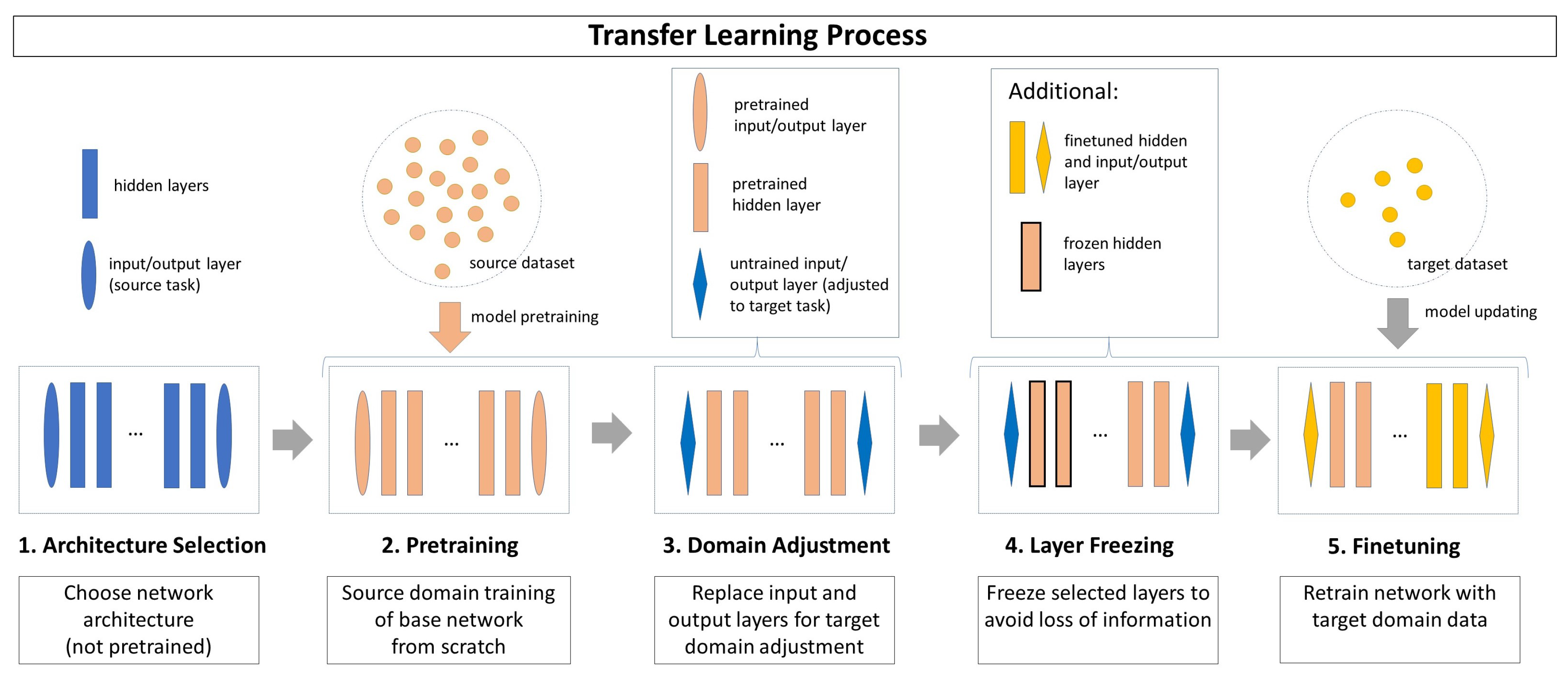
- Step 1 (Architecture Selection): An untrained network architecture is selected, whose hidden layer structure is assumed to solve both the source task and the target task. The input and output layers are chosen to fit the source task and source domain.
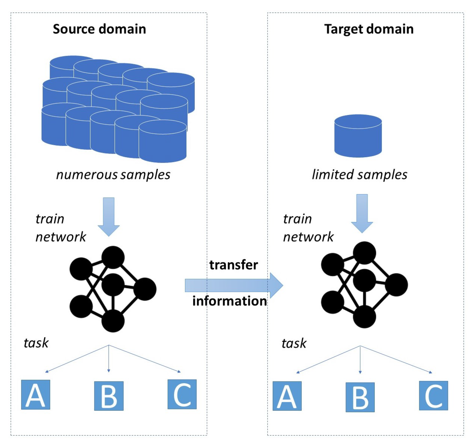
- Step 2 (Pretraining): The network is trained with the source domain dataset on the source task. Usually, the source dataset is expected to contain a high number of samples to make the training effective.
- Step 3 (Domain Adjustment): The pretrained network is adjusted to the target domain and target task, whereas the knowledge found in its hidden layers is preserved. To achieve this, only the input and output layers are replaced by untrained layers adapting the network to the target task and target domain.
- Step 4 (Layer Freezing): Depending on the TL strategy, some or all hidden layers can be frozen before training for the target task. The parameters of a frozen layer are not updated in future training processes, which ensures that the knowledge learned during source domain training is preserved. As a drawback, the adaptation ability of the target domain data is limited.
- Step 5 (Finetuning): The network is retrained on the target task with the target domain dataset. Usually, the target dataset has only a limited number of instances. The resulting model includes information from both the source domain and the target domain.
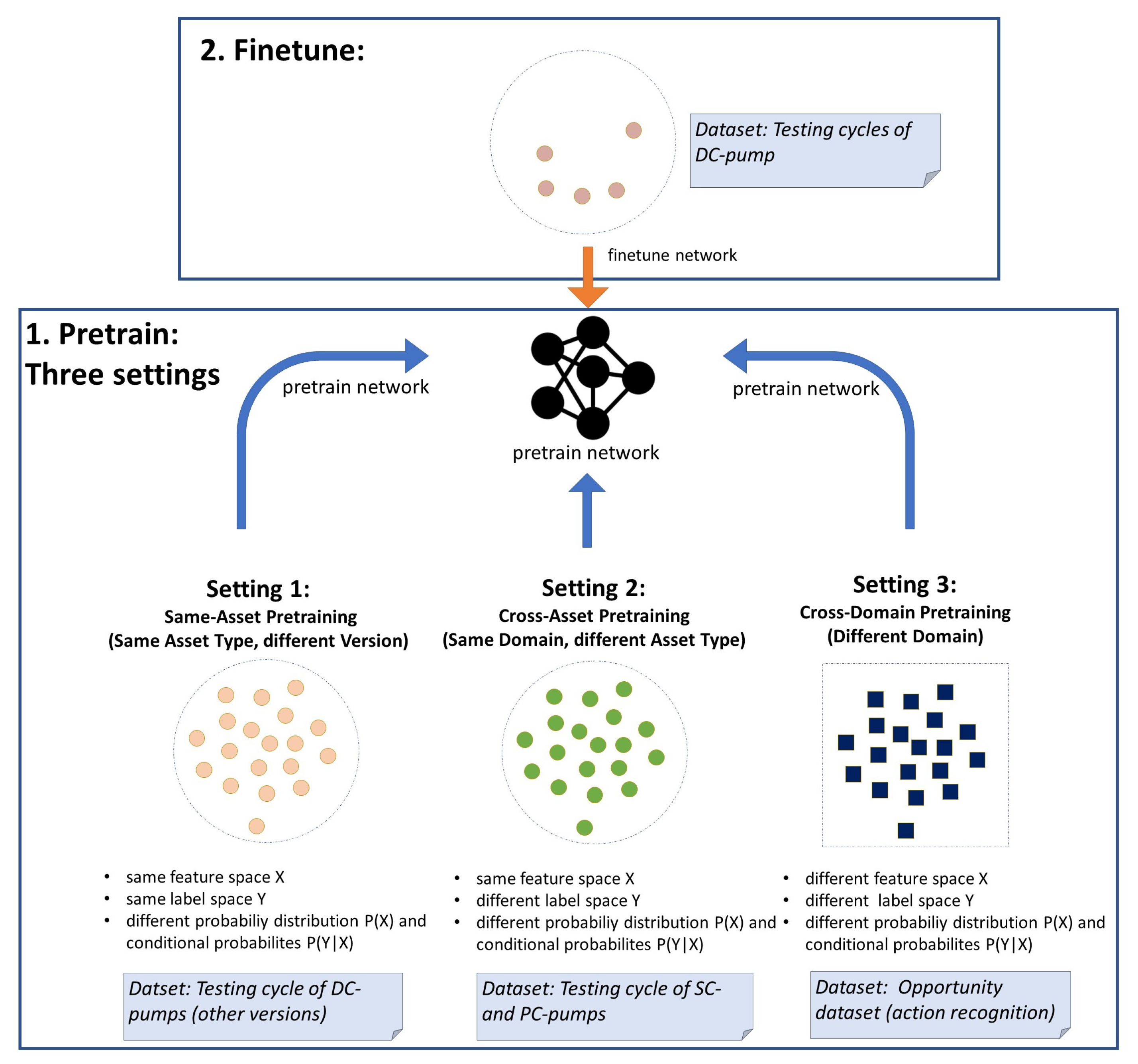
- Setting 1: Target domain and source domain share the same feature space X, and target task and source task share the same label space Y. However, the domains differ in terms of probability distribution of the feature space, while the tasks differ in the feature–label relationship (conditional probability ).
- Setting 2: In addition to non-identical probability distributions and non-identical conditional probabilities , the label space Y of the source task and the target task differs as well. Only the feature space X of both domains is identical in this setting.
- Setting 3: All four elements (feature space X, label space Y, feature probability distribution , and conditional probability ) differ between source domain and target domain as well as source task and target task.
3.2. Overview of Used Datasets
- (1)
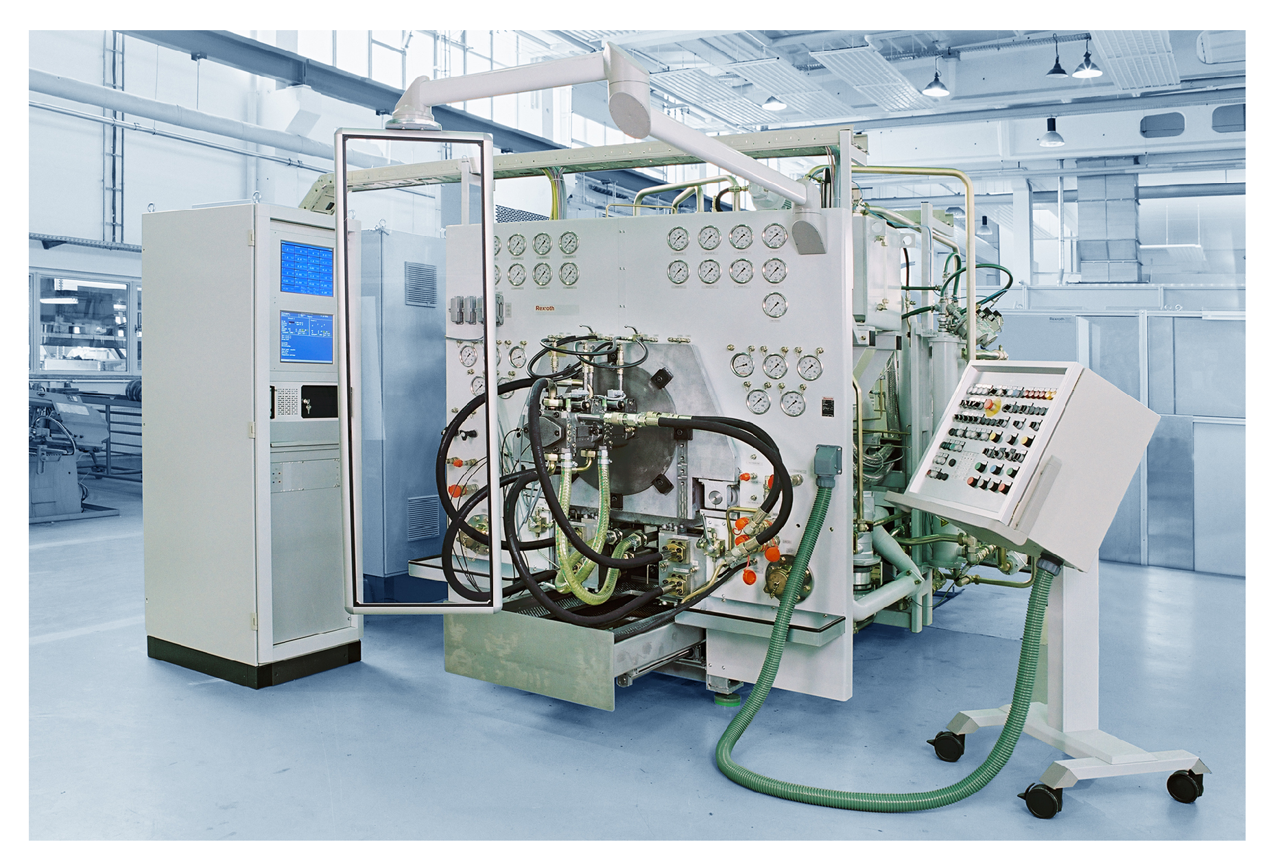
- Hydraulic Pump End-of-Line Dataset
- Direct control pumps (DC): 120 instances distributed over three versions (V35, V36, V38) differing in size and technical specifications with 40 instances each.
- Speed-based (mechanical) control pumps (SC): 38 instances
- Proportional control pumps (PC): 40 instances
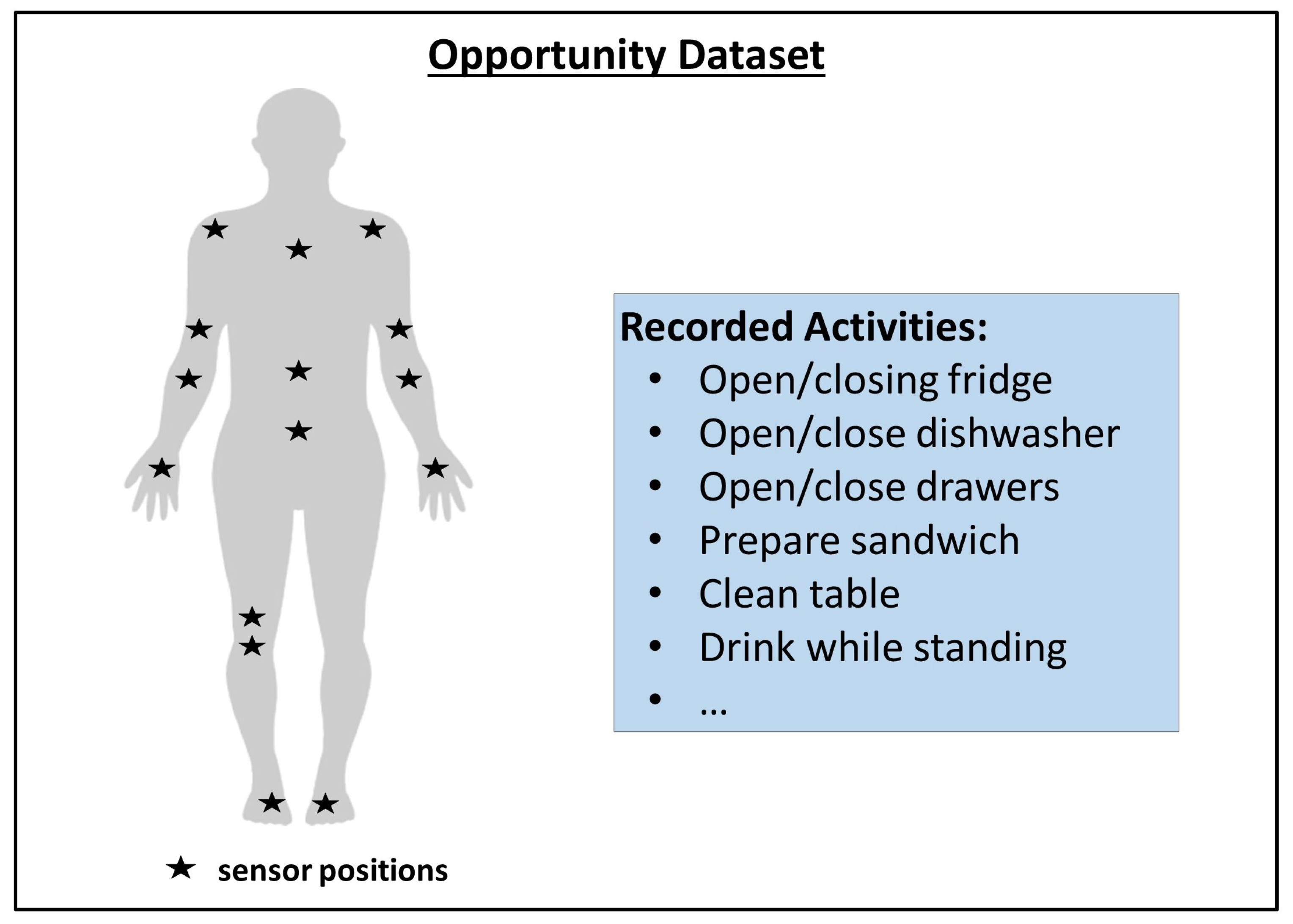
- (2)
- Opportunity Dataset
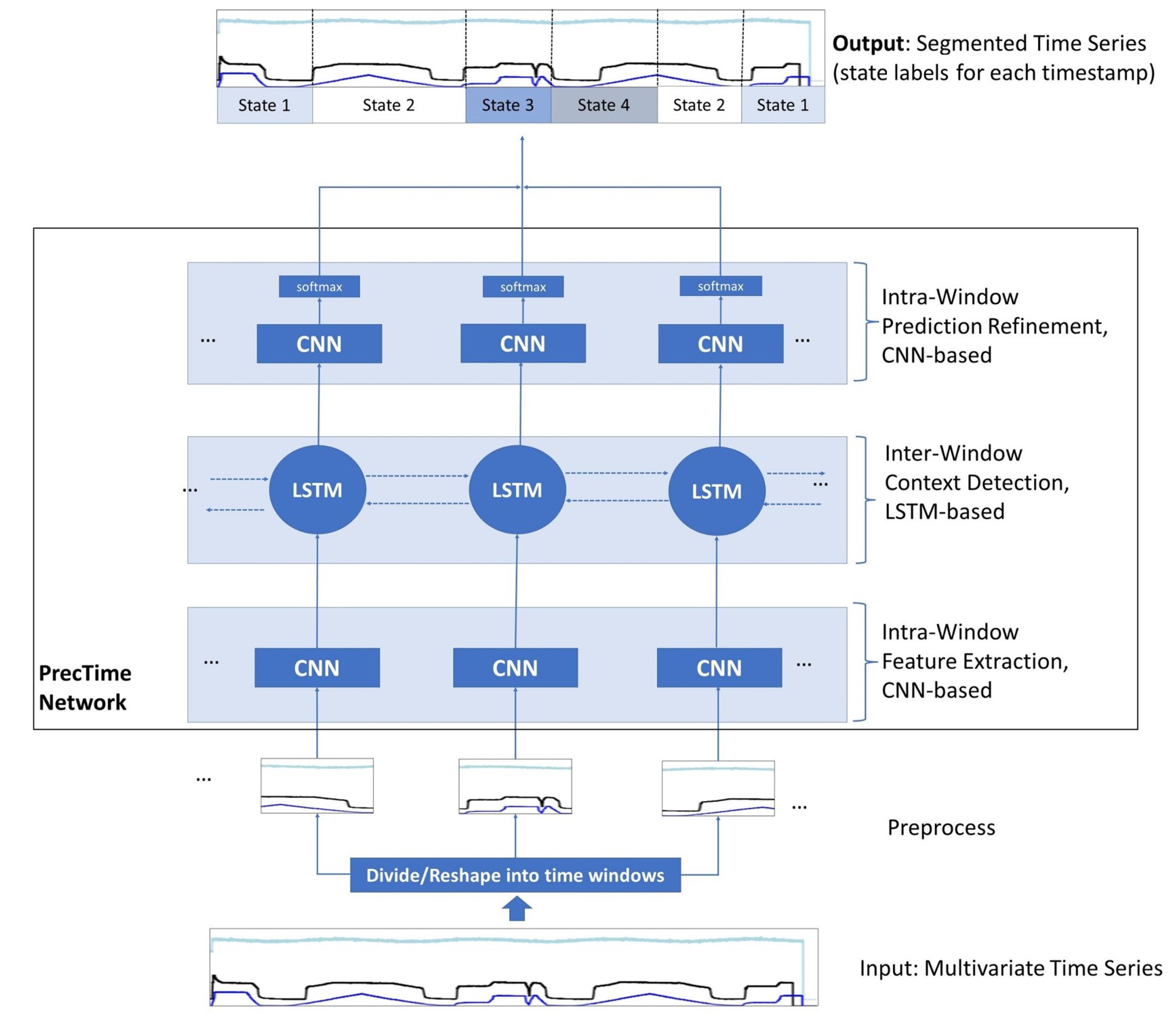
3.3. Model Architecture
3.4. Experimental Setup
- Setting 1 (Same-Asset Pretraining): Source data closely related to target data
- Setting 2 (Cross-Asset Pretraining): Source data distantly related to target data
- Setting 3 (Cross-Domain Pretraining): Source data non-related to target data
3.5. Implementation Details
4. Results and Discussion
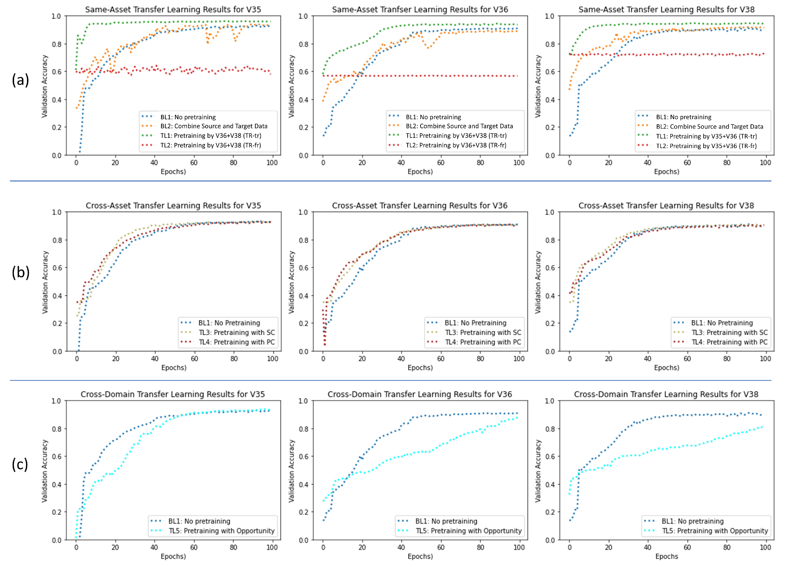
4.1. Results for Setting 1: Same-Asset Pretraining
4.2. Results for Setting 2: Cross-Asset Pretraining
4.3. Results for Setting 3: Cross-Domain Pretraining
5. Conclusions
Author Contributions
Funding
Institutional Review Board Statement
Informed Consent Statement
Data Availability Statement
Conflicts of Interest
Abbreviations
| ADL | activities of daily life |
| BL1 | baseline 1 |
| BL2 | baseline 2 |
| CNN | convolutional neural network |
| DC | direct control |
| HPEoL | hydraulic pump end-of-line |
| LSTM | long short-term memory |
| ML | machine learning |
| PC | proportional control |
| SC | speed-based control |
| TL | transfer learning |
| TSS | time series segmentation |
References
- Kaveh, A.; Talatahari, S.; Khodadadi, N. Stochastic Paint Optimizer: Theory and application in civil engineering. Eng. Comput. 2022, 38, 1921–1952. [Google Scholar] [CrossRef]
- Hoppenstedt, B.; Pryss, R.; Stelzer, B.; Meyer-Brötz, F.; Kammerer, K.; Treß, A.; Reichert, M. Techniques and Emerging Trends for State of the Art Equipment Maintenance Systems—A Bibliometric Analysis. Appl. Sci. 2018, 8, 916. [Google Scholar] [CrossRef]
- Hoppenstedt, B.; Reichert, M.; Kammerer, K.; Probst, T.; Schlee, W.; Spiliopoulou, M.; Pryss, R. Dimensionality Reduction and Subspace Clustering in Mixed Reality for Condition Monitoring of High-Dimensional Production Data. Sensors 2019, 19, 3303. [Google Scholar] [CrossRef]
- Kammerer, K.; Hoppenstedt, B.; Pryss, R.; Stökler, S.; Allgaier, J.; Reichert, M. Anomaly Detections for Manufacturing Systems Based on Sensor Data–Insights into Two Challenging Real-World Production Settings. Sensors 2019, 19, 5370. [Google Scholar] [CrossRef]
- Phan, H.; Andreotti, F.; Cooray, N.; Chén, O.; de Vos, M. SeqSleepNet: End-to-End Hierarchical Recurrent Neural Network for Sequence-to-Sequence Automatic Sleep Staging. IEEE Trans. Neural Syst. Rehabil. Eng. 2018, 27, 400–410. [Google Scholar] [CrossRef] [PubMed]
- Gaugel, S.; Reichert, M. PrecTime: A Deep Learning Architecture for Precise Time Series Segmentation in Industrial Manufacturing Operations, PrePrint. Available online: www.academia.edu (accessed on 22 February 2023).
- Lu, N.; Hu, H.; Yin, T.; Lei, Y.; Wang, S. Transfer Relation Network for Fault Diagnosis of Rotating Machinery with Small Data. IEEE Trans. Cybern. 2021, 52, 11927–11941. [Google Scholar] [CrossRef]
- Cao, P.; Zhang, S.; Tang, J. Preprocessing-Free Gear Fault Diagnosis Using Small Datasets With Deep Convolutional Neural Network-Based Transfer Learning. IEEE Access 2018, 6, 26241–26253. [Google Scholar] [CrossRef]
- Matias, P.; Folgado, D.; Gamboa, H.; Carreiro, A. Time Series Segmentation Using Neural Networks with Cross-Domain Transfer Learning. Electronics 2021, 10, 1805. [Google Scholar] [CrossRef]
- Zhuang, F.; Qi, Z.; Duan, K.; Xi, D.; Zhu, Y.; Zhu, H.; Xiong, H.; He, Q. A Comprehensive Survey on Transfer Learning. Proc. IEEE 2021, 109, 43–76. [Google Scholar] [CrossRef]
- Weber, M.; Auch, M.; Doblander, C.; Mandl, P.; Jacobsen, H.A. Transfer Learning With Time Series Data: A Systematic Mapping Study. IEEE Access 2021, 9, 165409–165432. [Google Scholar] [CrossRef]
- Maschler, B.; Weyrich, M. Deep Transfer Learning for Industrial Automation: A Review and Discussion of New Techniques for Data-Driven Machine Learning. IEEE Ind. Electron. Mag. 2021, 15, 65–75. [Google Scholar] [CrossRef]
- Li, W.; Gao, H.; Su, Y.; Momanyi, B.M. Unsupervised Domain Adaptation for Remote Sensing Semantic Segmentation with Transformer. Remote Sens. 2022, 14, 4942. [Google Scholar] [CrossRef]
- Liu, X.; Yoo, C.; Xing, F.; Oh, H.; Fakhri, G.; Kang, J.W.; Woo, J. Deep Unsupervised Domain Adaptation: A Review of Recent Advances and Perspectives. APSIPA Trans. Signal Inf. Process. 2022, 11, e25. [Google Scholar] [CrossRef]
- Heistracher, C.; Jalali, A.; Strobl, I.; Suendermann, A.; Meixner, S.; Holly, S.; Schall, D.; Haslhofer, B.; Kemnitz, J. Transfer Learning Strategies for Anomaly Detection in IoT Vibration Data. In Proceedings of the IECON 2021—47th Annual Conference of the IEEE Industrial Electronics Society, IEEE, Toronto, ON, Canada, 13–16 October 2021; pp. 1–6. [Google Scholar] [CrossRef]
- He, Q.Q.; Pang, P.C.I.; Si, Y.W. Multi-source Transfer Learning with Ensemble for Financial Time Series Forecasting. In Proceedings of the 2020 IEEE/WIC/ACM International Joint Conference on Web Intelligence and Intelligent Agent Technology (WI-IAT), Melbourne, Australia, 14–17 December 2021; pp. 227–233. [Google Scholar] [CrossRef]
- Yan, J.; Wang, L.; He, H.; Liang, D.; Song, W.; Han, W. Large-Area Land-Cover Changes Monitoring With Time-Series Remote Sensing Images Using Transferable Deep Models. IEEE Trans. Geosci. Remote Sens. 2022, 60, 4409917. [Google Scholar] [CrossRef]
- Lian, R.; Tan, H.; Peng, J.; Li, Q.; Wu, Y. Cross-Type Transfer for Deep Reinforcement Learning Based Hybrid Electric Vehicle Energy Management. IEEE Trans. Veh. Technol. 2020, 69, 8367–8380. [Google Scholar] [CrossRef]
- Aldayel, M.S.; Ykhlef, M.; Al-Nafjan, A.N. Electroencephalogram-Based Preference Prediction Using Deep Transfer Learning. IEEE Access 2020, 8, 176818–176829. [Google Scholar] [CrossRef]
- Gross, J.; Buettner, R.; Baumgartl, H. Benchmarking Transfer Learning Strategies in Time-Series Imaging: Recommendations for Analyzing Raw Sensor Data. IEEE Access 2022, 10, 16977–16991. [Google Scholar] [CrossRef]
- Wen, T.; Keyes, R. Time Series Anomaly Detection Using Convolutional Neural Networks and Transfer Learning. arXiv 2019, arXiv:1905.13628. [Google Scholar] [CrossRef]
- Gikunda, P.; Jouandeau, N. Homogeneous Transfer Active Learning for Time Series Classification. In Proceedings of the 2021 20th IEEE International Conference on Machine Learning and Applications (ICMLA), Pasadena, CA, USA, 13–16 December 2021; pp. 778–784. [Google Scholar] [CrossRef]
- Warushavithana, M.; Mitra, S.; Arabi, M.; Breidt, J.; Pallickara, S.L.; Pallickara, S. A Transfer Learning Scheme for Time Series Forecasting Using Facebook Prophet. In Proceedings of the 2021 IEEE International Conference on Cluster Computing (CLUSTER), Portland, OR, USA, 7–10 September 2021; pp. 809–810. [Google Scholar] [CrossRef]
- Fawaz, H.I.; Forestier, G.; Weber, J.; Idoumghar, L.; Muller, P.A. Transfer learning for time series classification. In Proceedings of the 2018 IEEE International Conference on Big Data (Big Data), Seattle, WA, USA, 10–13 December 2018; pp. 1367–1376. [Google Scholar]
- Dridi, A.; Afifi, H.; Moungla, H.; Boucetta, C. Transfer Learning for Classification and Prediction of Time Series for Next Generation Networks. In Proceedings of the ICC 2021—IEEE International Conference on Communications, Montreal, QC, Canada, 14–23 June 2021; pp. 1–6. [Google Scholar] [CrossRef]
- Yao, R.; Lin, G.; Shi, Q.; Ranasinghe, D. Efficient Dense Labeling of Human Activity Sequences from Wearables using Fully Convolutional Networks. Pattern Recognit. 2018, 78, 252–266. [Google Scholar] [CrossRef]
- Maschler, B.; Vietz, H.; Jazdi, N.; Weyrich, M. Continual Learning of Fault Prediction for Turbofan Engines using Deep Learning with Elastic Weight Consolidation. In Proceedings of the 2020 25th IEEE International Conference on Emerging Technologies and Factory Automation (ETFA), Vienna, Austria, 8–11 September 2020; pp. 959–966. [Google Scholar] [CrossRef]
- Kammerer, K.; Pryss, R.; Reichert, M. Context-Aware Querying and Injection of Process Fragments in Process-Aware Information Systems. In Proceedings of the 2020 IEEE 24th International Enterprise Distributed Object Computing Conference (EDOC), Eindhoven, The Netherlands, 5–8 October 2020; pp. 107–114. [Google Scholar] [CrossRef]
- Maschler, B.; Knodel, T.; Weyrich, M. Towards Deep Industrial Transfer Learning for Anomaly Detection on Time Series Data. In Proceedings of the 2021 26th IEEE International Conference on Emerging Technologies and Factory Automation (ETFA), Vasteras, Sweden, 7–10 September 2021; pp. 1–8. [Google Scholar] [CrossRef]
- Tercan, H.; Guajardo, A.; Meisen, T. Industrial Transfer Learning: Boosting Machine Learning in Production. In Proceedings of the 2019 IEEE 17th International Conference on Industrial Informatics (INDIN), IEEE, Helsinki, Finland, 22–25 July 2019; pp. 274–279. [Google Scholar] [CrossRef]
- Zhou, X.; Zhai, N.; Li, S.; Shi, H. Time Series Prediction Method of Industrial Process with Limited Data Based on Transfer Learning. IEEE Trans. Ind. Inform. 2022, 1–10. [Google Scholar] [CrossRef]
- Xu, W.; Wan, Y.; Zuo, T.Y.; Sha, X.M. Transfer Learning Based Data Feature Transfer for Fault Diagnosis. IEEE Access 2020, 8, 76120–76129. [Google Scholar] [CrossRef]
- Wu, S.; Jing, X.Y.; Zhang, Q.; Wu, F.; Zhao, H.; Dong, Y. Prediction Consistency Guided Convolutional Neural Networks for Cross-Domain Bearing Fault Diagnosis. IEEE Access 2020, 8, 120089–120103. [Google Scholar] [CrossRef]
- Xu, G.; Liu, M.; Jiang, Z.; Shen, W.; Huang, C. Online Fault Diagnosis Method Based on Transfer Convolutional Neural Networks. IEEE Trans. Instrum. Meas. 2020, 69, 509–520. [Google Scholar] [CrossRef]
- He, Y.; Tang, H.; Ren, Y. A Multi-channel Transfer Learning Framework for Fault Diagnosis of Axial Piston Pump. In Proceedings of the 2021 Global Reliability and Prognostics and Health Management (PHM-Nanjing), Nanjing, China, 15–17 October 2021; pp. 1–7. [Google Scholar] [CrossRef]
- Lin, Y.P.; Jung, T.P. Improving EEG-Based Emotion Classification Using Conditional Transfer Learning. Front. Hum. Neurosci. 2017, 11, 334. [Google Scholar] [CrossRef]
- Sun, S.; Shi, H.; Wu, Y. A survey of multi-source domain adaptation. Inf. Fusion 2015, 24, 84–92. [Google Scholar] [CrossRef]
- Chambers, R.D.; Yoder, N.C. FilterNet: A Many-to-Many Deep Learning Architecture for Time Series Classification. Sensors 2020, 20, 2498. [Google Scholar] [CrossRef] [PubMed]
- Chavarriaga, R.; Sagha, H.; Bayati, H.; Millan, J.d.R.; Roggen, D.; Förster, K.; Calatroni, A.; Tröster, G.; Lukowicz, P.; Bannach, D.; et al. Robust activity recognition for assistive technologies: Benchmarking machine learning techniques. In Proceedings of the Workshop on Machine Learning for Assistive Technologies at the Twenty-Fourth Annual Conference on Neural Information Processing Systems (NIPS-2010), Whistler, BC, Canada, 10 December 2010. [Google Scholar]


| Number of Training Samples in Target Data | V35 as Target Data V36 + V38 as Source | V36 as Target Data V35 + V38 as Source | V38 as Target Data V35 + V36 as Source | |||||||||
|---|---|---|---|---|---|---|---|---|---|---|---|---|
| BL1 | BL2 | TL-fr | TL-tr | BL1 | BL2 | TL-fr | TL-tr | BL1 | BL2 | TL-fr | TL-tr | |
| 1 | 59.0 | 45.2 | 53.0 | 93.8 | 66.9 | 45.0 | 50.3 | 86.0 | 77.1 | 83.9 | 69.2 | 88.7 |
| 3 | 92.3 | 92.5 | 57.8 | 95.9 | 90.9 | 88.9 | 56.8 | 93.5 | 90.2 | 91.3 | 73.0 | 94.4 |
| 5 | 94.3 | 92.5 | 53.5 | 96.9 | 92.5 | 92.5 | 60.2 | 95.5 | 90.4 | 93.1 | 70.7 | 95.8 |
| 10 | 95.7 | 97.0 | 58.4 | 97.4 | 94.1 | 95.2 | 59.3 | 96.7 | 93.1 | 96.3 | 69.0 | 96.5 |
| Setting | V38 as Target Dataset | V36 as Target Dataset | V35 as Target Dataset |
|---|---|---|---|
| BL1 (no pretraining) | 90.2 | 91.0 | 92.4 |
| Pretraining by SC pump dataset | 90.8 | 90.5 | 92.9 |
| Pretraining by PC pump dataset | 90.4 | 90.8 | 92.4 |
| Setting No. | Setting Description | Effect on Asymptote | Effect on Training Start | Effect on Training Slope |
|---|---|---|---|---|
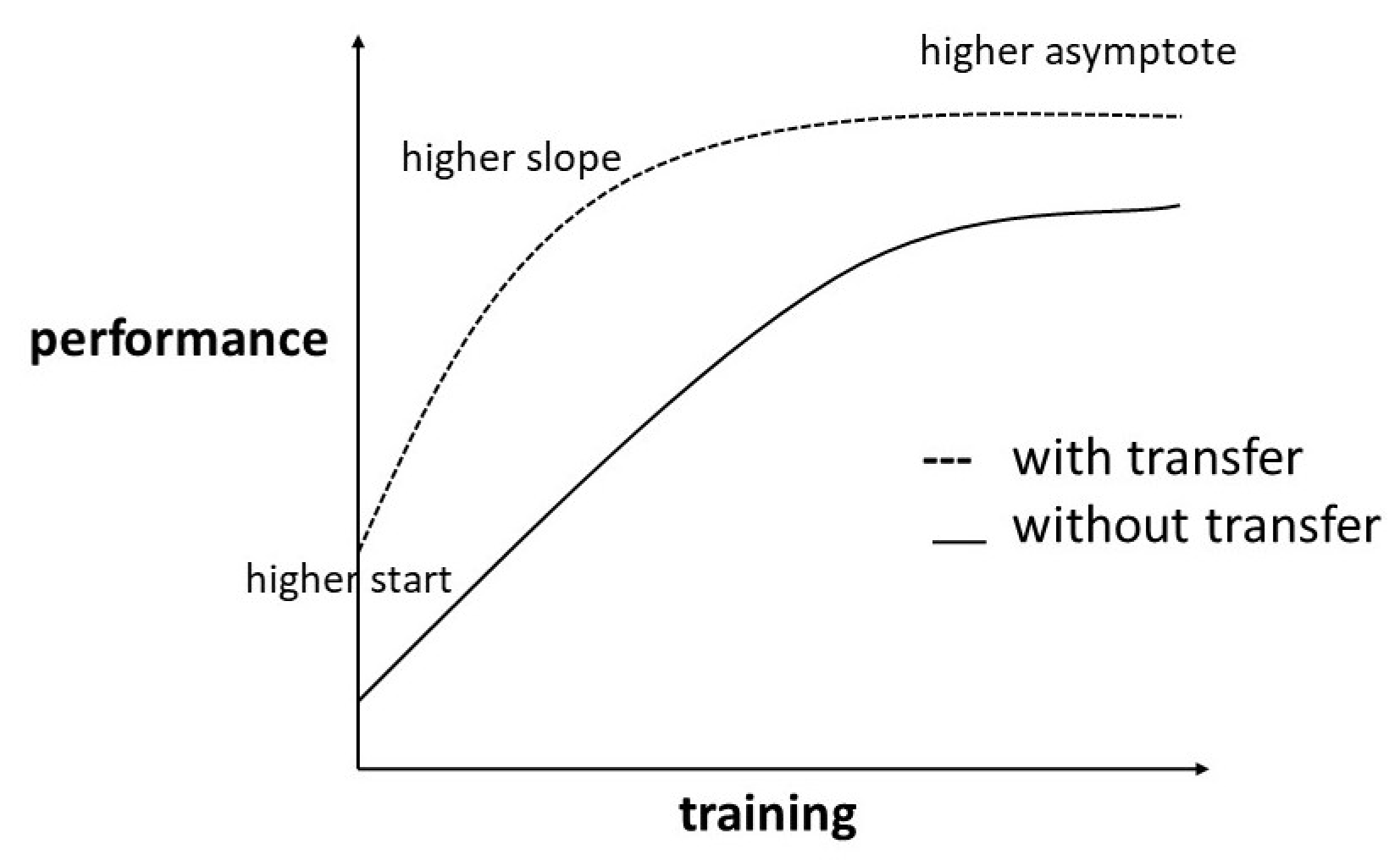
| 1 | Same-asset pretraining (closely related source and target data) | + | ++ | + |
| 2 | Cross-asset pretraining (distantly related source and target data) | 0 | + | + |
| 3 | Cross-domain pretraining (non-related source and target data) | 0 | 0 | - |
Disclaimer/Publisher’s Note: The statements, opinions and data contained in all publications are solely those of the individual author(s) and contributor(s) and not of MDPI and/or the editor(s). MDPI and/or the editor(s) disclaim responsibility for any injury to people or property resulting from any ideas, methods, instructions or products referred to in the content. |
© 2023 by the authors. Licensee MDPI, Basel, Switzerland. This article is an open access article distributed under the terms and conditions of the Creative Commons Attribution (CC BY) license (https://creativecommons.org/licenses/by/4.0/).
Share and Cite
Gaugel, S.; Reichert, M. Industrial Transfer Learning for Multivariate Time Series Segmentation: A Case Study on Hydraulic Pump Testing Cycles. Sensors 2023, 23, 3636. https://doi.org/10.3390/s23073636
Gaugel S, Reichert M. Industrial Transfer Learning for Multivariate Time Series Segmentation: A Case Study on Hydraulic Pump Testing Cycles. Sensors. 2023; 23(7):3636. https://doi.org/10.3390/s23073636
Chicago/Turabian StyleGaugel, Stefan, and Manfred Reichert. 2023. "Industrial Transfer Learning for Multivariate Time Series Segmentation: A Case Study on Hydraulic Pump Testing Cycles" Sensors 23, no. 7: 3636. https://doi.org/10.3390/s23073636
APA StyleGaugel, S., & Reichert, M. (2023). Industrial Transfer Learning for Multivariate Time Series Segmentation: A Case Study on Hydraulic Pump Testing Cycles. Sensors, 23(7), 3636. https://doi.org/10.3390/s23073636