1. Introduction
Significant advances in deep-learning technology have made it possible to automate and accelerate various tasks. In particular, image classification has been put to practical use in a variety of applications, such as face recognition and anomaly detection. In addition, cloud services have become popular among common organizations and individuals for the purpose of reducing costs, facilitating data sharing, and so on. For these reasons, image classification tasks are increasingly being accomplished through cloud servers. To utilize a model on a cloud server, a user should transmit test images to the server.
However, cloud servers are generally not reliable, and thus test images are under threat of being compromised outside of the servers. As a result, the copyright and privacy information in the test images might be disclosed to third parties. Additionally, the user generally needs to classify a large number of images; in other words, a large amount of image data should be transmitted to the server in succession. Therefore, it is desirable to minimize the data amount of the test images.
Many compression methods have been proposed to reduce the data amount of images. Compression methods can be classified into two categories: lossless and lossy methods. In general, lossy methods can more efficiently reduce the data amount compared with lossless methods. A typical lossy method is JPEG, which is one of the image compression standards. On the basis of human visual features, JPEG compression significantly reduces the information of high-frequency components and commonly applies 4:2:0 downsampling, i.e., horizontal and vertical downsampling of chrominance. Consequently, we can notably reduce the data amount while preserving high image quality. It is noted that JPEG compression can adjust the image quality and data amount by varying the quality factor.
In recent years, there has been a great amount of effort to develop secure image-classification systems with copyright and privacy protection for images. Federated learning is one technique that can be used in developing such systems [
1,
2,
3]. Multiple clients individually train a single model by using their own data, while a central server integrates the parameters trained by each client. This technique can protect training images but not test images. On another front, secure computation is also drawing attention. This technique can directly adapt computational operations to encrypted data. A large number of methods have been proposed that automatically classify data encrypted with secure computation [
4,
5,
6]. These methods can protect test data; however, the encrypted data can hardly be compressed. Even if the encrypted data is successfully compressed, it is difficult to decrypt the data.
Another approach for protecting copyright and privacy information in test images is to conceal the visual information. Image encryption is a typical technique for concealing visual information, and image-encryption methods have been actively studied to train encrypted images using deep neural networks [
3,
7,
8,
9,
10,
11,
12,
13,
14,
15,
16,
17]. The method in [
3] combines federated learning with image encryption for test images. Encrypted image classification via a cloud server assumes that a user encrypts test images and transmits the encrypted images to a server. Thus, it is desirable to be able to compress the encrypted images in terms of the transmission efficiency; however, most such methods [
3,
9,
10,
11,
12,
13,
14,
15,
16] do not consider image compression. Aprilpyone et al. employed the encryption-then-compression (EtC) system [
18] as an image encryption algorithm so that the encrypted images (hereafter, EtC images) possess a high compression performance [
8]. Some other methods protect visual information using machine learning instead of encryption and classify protected images [
19,
20]. The methods [
8,
9,
10,
11,
12,
13,
14,
15,
19,
20], however, degrade the classification accuracy due to the protection of visual information.
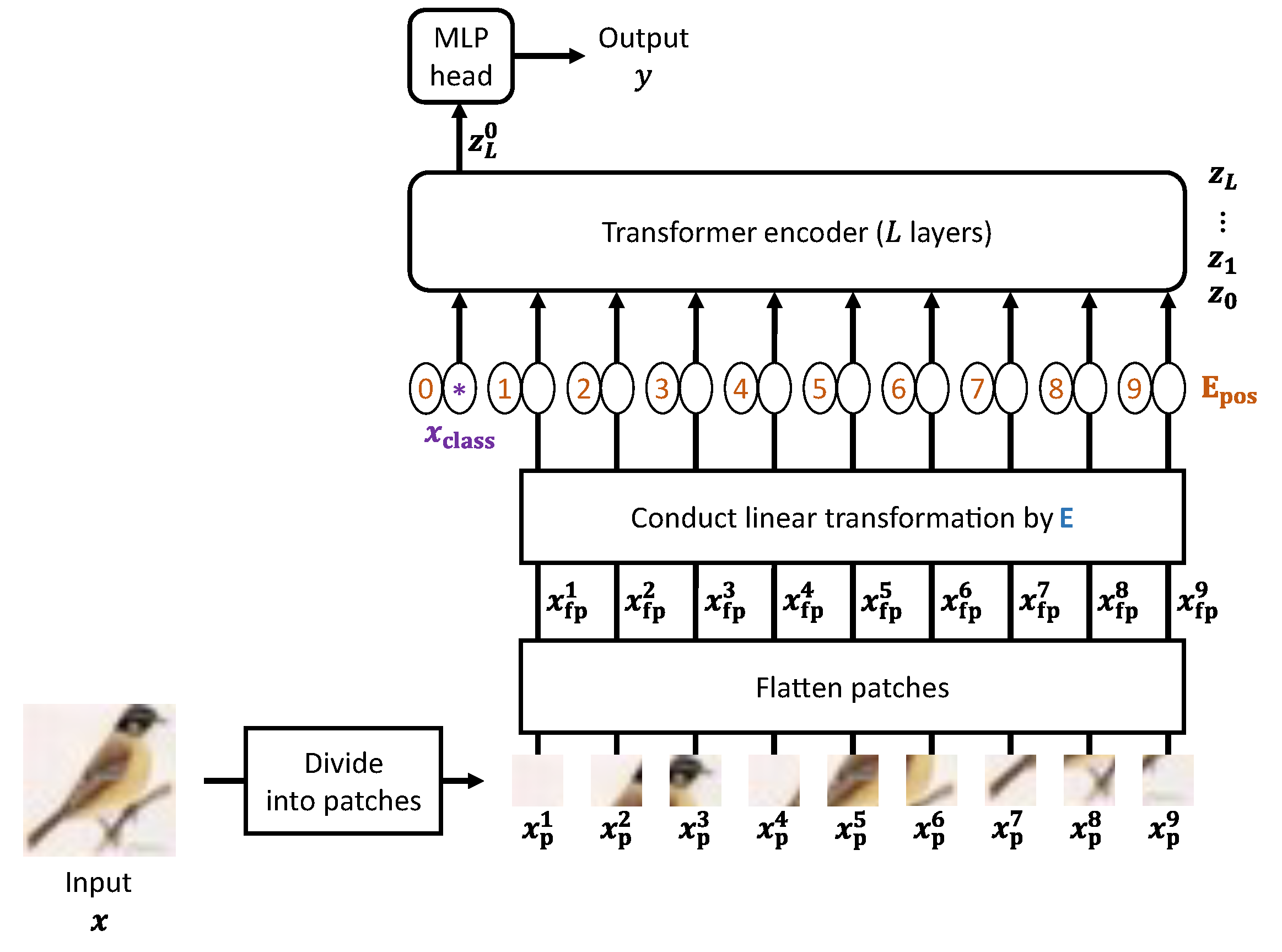
The method in [
8] employs the Vision Transformer (ViT) [
21] and ConvMixer [
22], which are called isotropic networks, as image-classification models. They are known to provide a higher classification accuracy compared with convolutional neural networks, which are the conventional mainstream image-classification models. Kiya et al. focused on the properties of ViT to maintain the classification accuracy for encrypted images [
16]. This method prepares a series of encryption keys (hereafter, key set) and uses it to encrypt not only test images but also a trained ViT model. The encrypted ViT model is eventually suitable for the encrypted images. This is the first study that perfectly preserves the classification accuracy for encrypted images. However, the image encryption process in this method employs a pixel-wise transformation, so the encrypted images can hardly be compressed.
As an extension of the method [
16], we previously introduced an EtC system for the image encryption process [
17]. The EtC system is based on a block-wise transformation, and thus the EtC images can maintain high compression performance. Further, this method does not cause any degradation to the classification accuracy for EtC images by using a model encryption algorithm that corresponds to the EtC system. Therefore, we not only successfully avoid any degradation to the classification accuracy but also compress the encrypted images. In [
17], we surveyed the performance of lossless compression using JPEG-LS [
23].
On the basis of our previous method [
17], this paper, for the first time, investigates the effects of JPEG compression, which is a widely used lossy compression standard, on the classification accuracy. In our experiments, we confirm that a high classification accuracy can be preserved even for JPEG-compressed EtC images. Moreover, this paper verifies the effectiveness of JPEG compression in terms of classification and compression performance compared with linear quantization.
In this paper, we demonstrate that JPEG noise added to the high-frequency component barely degrades the accuracy of ViT classification. To the best of our knowledge, this is the only study that successfully compresses encrypted images using the JPEG lossy standard and classifies the compressed encrypted-images with very little degradation to accuracy. Through a series of studies, we reach the conclusion that compressed EtC images can be classified without degradation to accuracy.
3. Evaluation of JPEG-Compression Effects on the Classification Results
This paper extends the previous method [
17] to verify the effects of JPEG compression for EtC images on the classification results. This section first outlines evaluation schemes to investigate the JPEG-compression effects and then details the image and model-encryption procedure. Finally, we describe the evaluation metrics in our experiments.
3.1. Overview
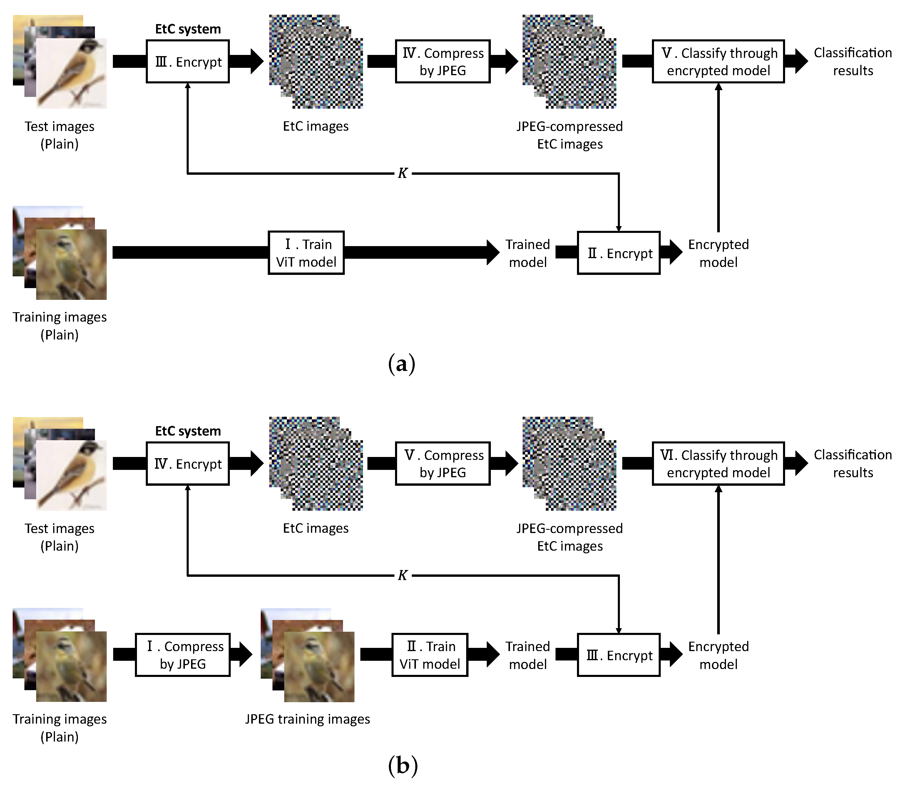
Figure 3 illustrates the flows of our evaluation schemes. We prepared two types of schemes to elaborately examine the effects of JPEG compression. Hereafter, the schemes shown in
Figure 3a,b will be called evaluation schemes A and B, respectively. Note that all images used in this paper have RGB color channels.
First, a ViT model is trained by using plain training images in scheme A. In scheme B, the plain training-images are preliminarily compressed by JPEG, and the ViT model is trained by using the compressed images (JPEG training images, hereafter). The flow after model training is the same between the two evaluation schemes. A trusted third-party encrypts the trained model with a key set
, and
K and the encrypted model are transmitted to a user and a provider, respectively. The user encrypts test images using the EtC system [
18] and compresses the EtC images by JPEG. The JPEG-compressed EtC images are then sent to the provider to be classified. The provider classifies each JPEG-compressed EtC image through the encrypted model and finally returns the classification results to the user.
In scheme A, test images encrypted by the EtC system are compressed by JPEG. Thus, we verify the compression effects for test images through comparison with our previous method [
17]. In comparison, both training and test images are compressed by JPEG in scheme B. Through a comparison between schemes A and B, we examine the compression effects for training images on the classification of JPEG-compressed test images.
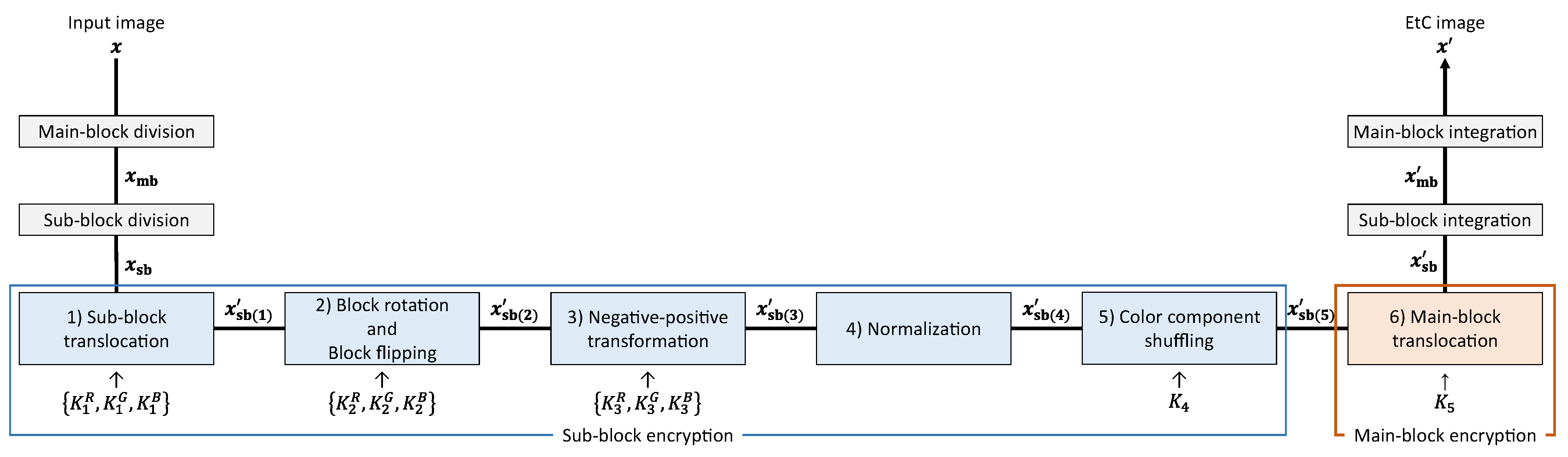
3.2. Image Encryption
Figure 4 shows an image-encryption procedure. This encryption algorithm is an extension of the block-based image-encryption method [
18], which is one of the EtC systems. We preliminarily prepare a key set
so as to encrypt an input image. Note that
,
, and
are key sets consisting of three keys
, and
and
represent single keys. The image-encryption procedure is described as follows.
- Step i-1:
Divide an input image into main blocks, and further divide each main block into sub blocks.
- Step i-2:
Translocate sub blocks within each main block using .
- Step i-3:
Rotate and flip each sub block using .
- Step i-4:
Apply a negative–positive transformation to each sub block using .
- Step i-5:
Normalize all pixels.
- Step i-6:
Shuffle the R, G, and B components in each sub block using .
- Step i-7:
Translocate main blocks using .
- Step i-8:
Integrate all of the sub and main blocks.
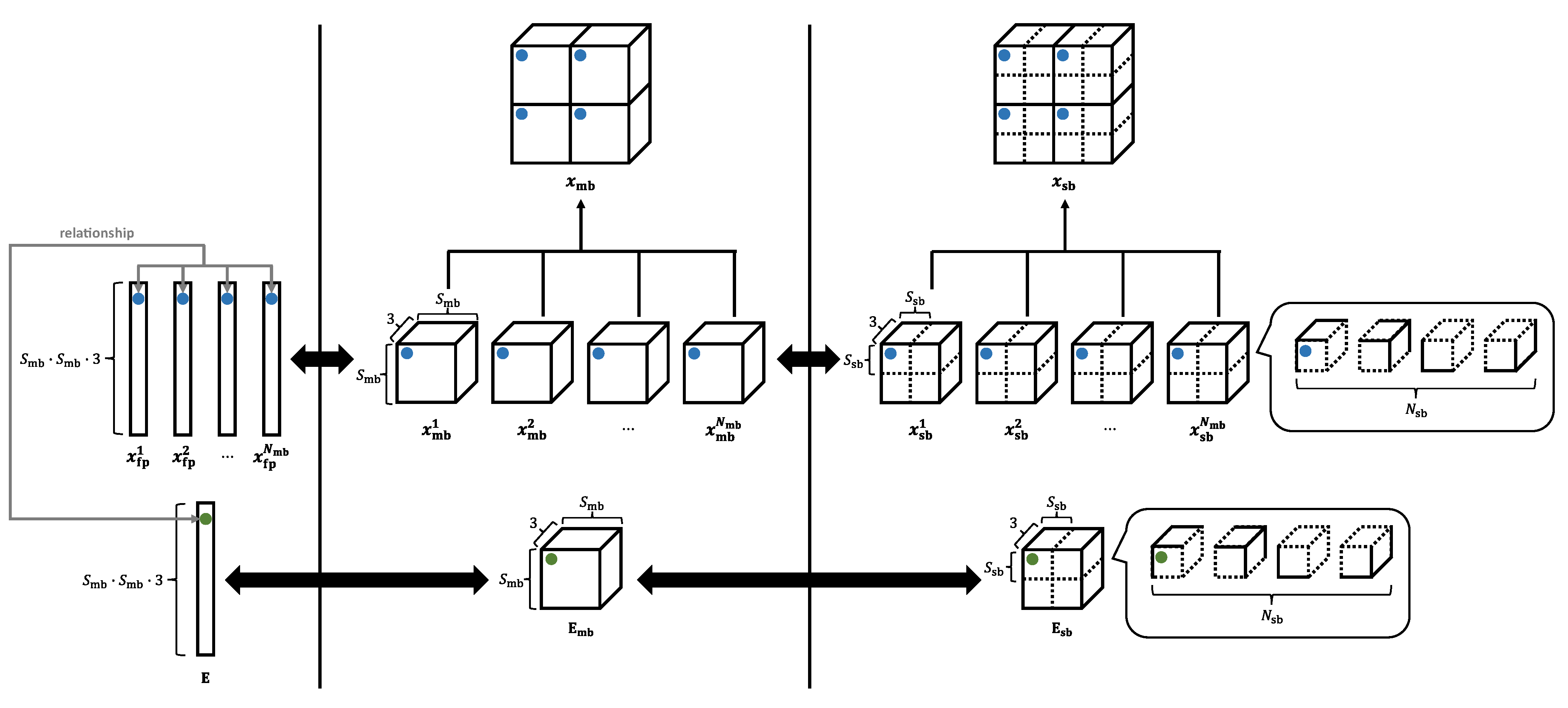
In Step i-1, the input image is divided into main and sub blocks as shown in
Figure 5. We call Steps i-2 to i-6 sub-block encryption and Step i-7 main-block encryption.
Sub-block encryption includes five operations. Each operation, except normalization, is a sub-block-wise transformation in each main block, and , , , and are shared among all the main blocks. consist of three single keys , , and corresponding to the R, G, and B components, respectively. Thus, each component can be transformed independently when , , and are different from each other. In contrast, all the components are transformed commonly when the three keys are identical.
The former is called independent transformation, and the latter is called common transformation in this paper. The main-block encryption consists of a single operation, where the main blocks are translocated. Since for the main-block encryption is not a key set but a single key, the R, G, and B components should be translocated commonly. The encryption algorithm transforms an input image while preserving the pixel-to-pixel correlation in each sub block, and so the encrypted image is expected to be highly compressed.
Before we detail the sub-block and main-block encryptions, symbols are preliminarily defined as follows.
H and W: the height and width of an image.
: an input image.
and : the main-block and sub-block sizes.
: the number of main blocks.
: the number of sub blocks within each main block.
: an image after main-block division, called a main-block image.
: an image after sub-block division, called a sub-block image.
: an image after the -th operation in sub-block encryption, where .
: an image after main-block encryption.
: an image after sub-block integration.
: an image after main-block integration, i.e., an EtC image.
, , and : pixel values in , , and , respectively.
- -
: a main-block number.
- -
: a sub-block number in the m-th main block.
- -
: a position in the height direction in the s-th sub block.
- -
: a position in the width direction in the s-th sub block.
- -
: a color-channel number.
3.2.1. Sub-Block Translocation
We first translocate sub blocks within each main block by using
. Vectors
are generated by
,
, and
, respectively. Each vector
is represented as
where
, and
if
. The second dimension of
denotes a sub-block number; thus, the sub blocks are translocated by replacing their numbers with
:
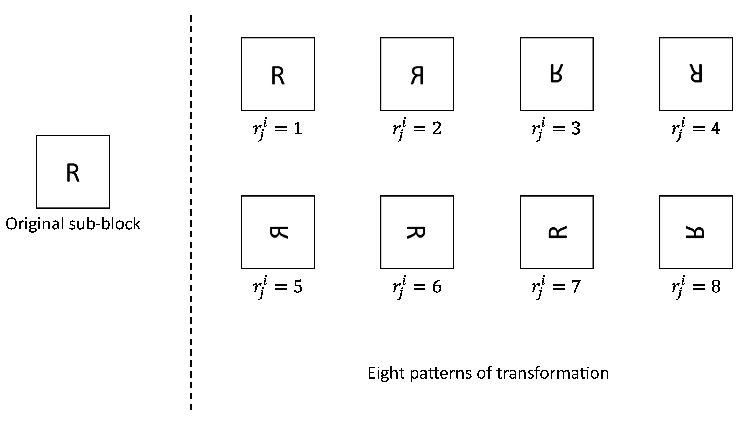
3.2.2. Block Rotation and Block Flipping
Next, we rotate and flip each sub block using
. As shown in
Figure 6, there are eight transformation patterns for each sub block. Three vectors
are derived from
,
, and
, respectively. Each vector
is denoted by
where
. The third and fourth dimensions of
represent the position in the height and width directions in each sub block, respectively. Therefore, each sub block is rotated and flipped by translocating pixels within the sub block depending on
:
where
, and
.
3.2.3. Negative–Positive Transformation
We then apply a negative–positive transformation to each sub block with
. Vectors
are generated using
,
, and
and given by
where
. The negative–positive transformation is conducted on the basis of
:
3.2.4. Normalization
All pixels in
should be normalized as
where
S is an arbitrary constant, while
in this paper. In the case of
in Equation (
10),
can be expressed as
Otherwise,
is given by
From Equations (
12) and (
13), it is clear that the negative–positive transformation with normalization can be regarded as an operation of retaining or flipping the sign of each pixel value. This property prevents a model encryption algorithm from being complex. We detail the algorithm in
Section 3.3.3.
3.2.5. Color Component Shuffling
We then shuffle the R, G, and B components in each sub block using
. A vector
is derived from
and represented as
where
. The fifth dimension of
denotes a color-channel number; this operation swaps pixel values among the color components according to
:
and
3.2.6. Main-Block Translocation
Finally, the main blocks are translocated with
. A vector
obtained by
is given by
where
, and
if
. The first dimension of
represents a main-block number, so we translocate the main blocks by replacing their numbers with
:
3.3. Model Encryption
This section describes the model-encryption procedure. While image encryption can protect visual information, it seriously deteriorates the classification accuracy. The model encryption in this paper not only cancels out the effects but also prevents unauthorized accesses to a trained ViT model by encryption.
We assume that the patch size
P in ViT is the same as the main-block size
in the image encryption and that the number of patches
N is equal to the number of main blocks
. The patch set
has
dimensions, and the main-block image
has
dimensions—namely,
and
are identical. Here, we define both
and
as a single main block, respectively. Note that
, and
N is equal to
, and so
is an index denoting the main-block number.
is a part of
without sub-block division, while
is a part of
with sub-block division. They are represented as
and
are identical, so the patch
and the main block
are treated as one and the same. Therefore,
obtained by flattening
is also derived from flattening
. Hereafter,
P and
N will be denoted as
and
, respectively, for the sake of consistency.
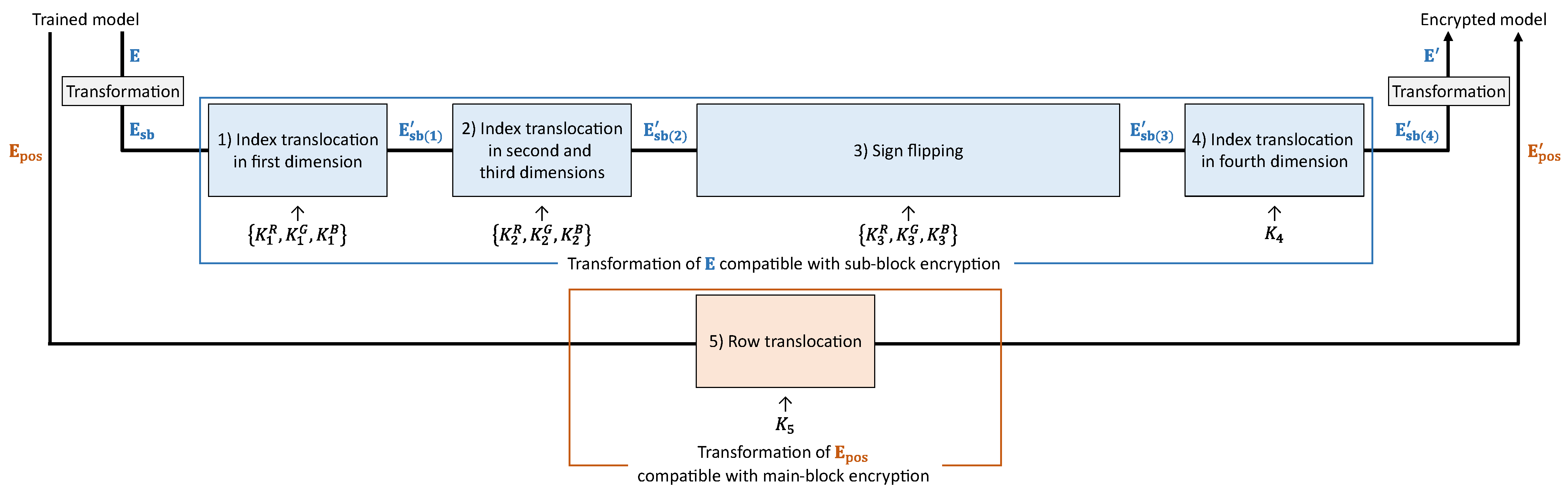
Figure 7 illustrates a model-encryption procedure. One of the purposes of model encryption is to ensure that the classification results are never affected by image encryption. Thus, we transform the parameters
and
in the trained model with the key set
K, which is the same as for the image encryption. Each operation in the model encryption is compatible with each operation in the image encryption. The model-encryption procedure is described as follows.
- Step m-1:
Transform to obtain .
- Step m-2:
Translocate indices in the first dimension of using .
- Step m-3:
Translocate indices in the second and third dimensions of using .
- Step m-4:
Flip or retain the signs of the elements in using .
- Step m-5:
Translocate indices in the fourth dimension of using .
- Step m-6:
Transform into the original dimension of to derive .
- Step m-7:
Translocate rows in using to obtain .
Figure 8 illustrates the relationship between a divided image and
. We transform
to
and then obtain
in Step m-1. This step allows
to be encrypted directly by using the vectors for the sub-block encryption.
As mentioned in
Section 2.1,
and
correspond to
and
, respectively. Each operation in the image encryption generally sacrifices their correspondence. Accordingly, the common image-encryption methods significantly degrade the classification accuracy. In contrast, an image-encryption method based on the EtC system is compatible with each parameter of ViT. Taking advantage of this compatibility, we proposed a model-encryption method for ViT without any degradation to the classification accuracy caused by image encryption [
17]. Our previous method demonstrated that the classification accuracy was never affected by encryption [
25].
We detail each operation in the model encryption below. Hereafter, , where , represents a parameter after the -th operation to . Further, and , where , denote the elements of and , respectively.
3.3.1. Index Translocation in the First Dimension
We first translocate indices in the first dimension of
. On the basis of Equation (
6), the sub-block translocation replaces the indices in the second dimension of
with vectors
derived using
. The second dimension of
corresponds to the first dimension of
. Thus, the indices in the first dimension of
should be translocated by replacing them with
:
3.3.2. Index Translocation in the Second and Third Dimensions
Next, we translocate indices in the second and third dimensions of
. As shown in Equation (
8), the block rotation and block flipping translocates the indices in the third and fourth dimensions of
in response to vectors
derived from
. The third and fourth dimensions of
are compatible with the second and third dimensions of
, respectively. The indices in the second and third dimensions of
should be translocated accordingly depending on
:
3.3.3. Sign Flipping
Here, we flip signs of the elements in
. As described in
Section 3.2.4, the negative–positive transformation with normalization is regarded as an operation to flip or retain the signs of the pixel values in
. We determine whether to flip or retain the signs of the elements in
responding to vectors
generated using
.
is consequently transformed as
3.3.4. Index Translocation in Fourth Dimension
We then translocate indices in the fourth dimension of
. As shown in Equations (
15)–(
17), the color component shuffling translocates the indices in the fifth dimension of
on the basis of the vector
derived using
. The fifth dimension of
corresponds to the fourth dimension of
. We, thus, translocate the indices in the fourth dimension of
by using
:
and
3.3.5. Row Translocation
Finally, we translocate rows in
. As shown in Equation (
19), the main-block translocation replaces the indices in the first dimension of
with vector
obtained by
. Both
and the first dimension of
represent the main-block number, and so the main-block translocation is regarded as an operation to replace
with
. To preserve the relationship between
and
, the rows in
should accordingly be translocated by using
as
where
and
denote the elements of
and
, respectively. Note that
is an index corresponding to the dimensions of
and
.
3.4. Evaluation Metrics
We verified the effectiveness of JPEG compression in terms of compression and classification performance. We calculated the average amount of image data to evaluate the compression performance. In addition, we prepared two metrics to assess the classification performance: the classification accuracy and change rate. In this paper, the change rate provides the percentage of difference between the classification results for plain test images with a plain trained model and those for target images with a target model. For instance, the target images and target model means JPEG-compressed EtC images and an encrypted model, respectively. In the case that the change rate indicates 0%, both classification results are identical.
For scheme A, shown in
Figure 3a, we provide five patterns for the quality factor (
Q): 100, 95, 90, 85, and 80. To compare the effects of JPEG compression, each metric was also calculated for EtC images compressed by linear quantization. In comparison, scheme B, shown in
Figure 3b, compressed both training images and EtC images by using JPEG with
. In common with scheme A, the classification accuracy was also calculated for the case of using linear quantization. Hereafter, the EtC images and the training images after the linear quantization are called quantized EtC images and quantized training images, respectively.
4. Experiments
In this section, the effects of JPEG compression are examined in terms of classification and compression performance by using the metrics described in
Section 3.4.
4.1. Experimental Setup
We used the CIFAR-10 dataset with 10 classes in this experiment. This dataset consists of 50,000 training images and 10,000 test images. All image sizes are pixels, while we preliminarily resized each image to pixels by using the bicubic interpolation method. All training and test images were stored in PPM format.
The ViT model is trained through two phases: pre-training and fine-tuning. In this experiment, we used a pre-trained ViT model using ImageNet-21k with a patch size . We then fine-tuned the pre-trained ViT model by using plain training images for scheme A or JPEG training images for scheme B. In both schemes, the ViT model was fine-tuned with a learning rate of 0.03 and an epoch of 5000.
In the image encryption, the main-block size
was defined as 16, which was the same as
P, while the sub-block size
was set to 8 or 16. Additionally, as mentioned in
Section 3.2, we could choose either the common or independent transformation in regard to color components. Consequently, four types of EtC images were generated for each test image.
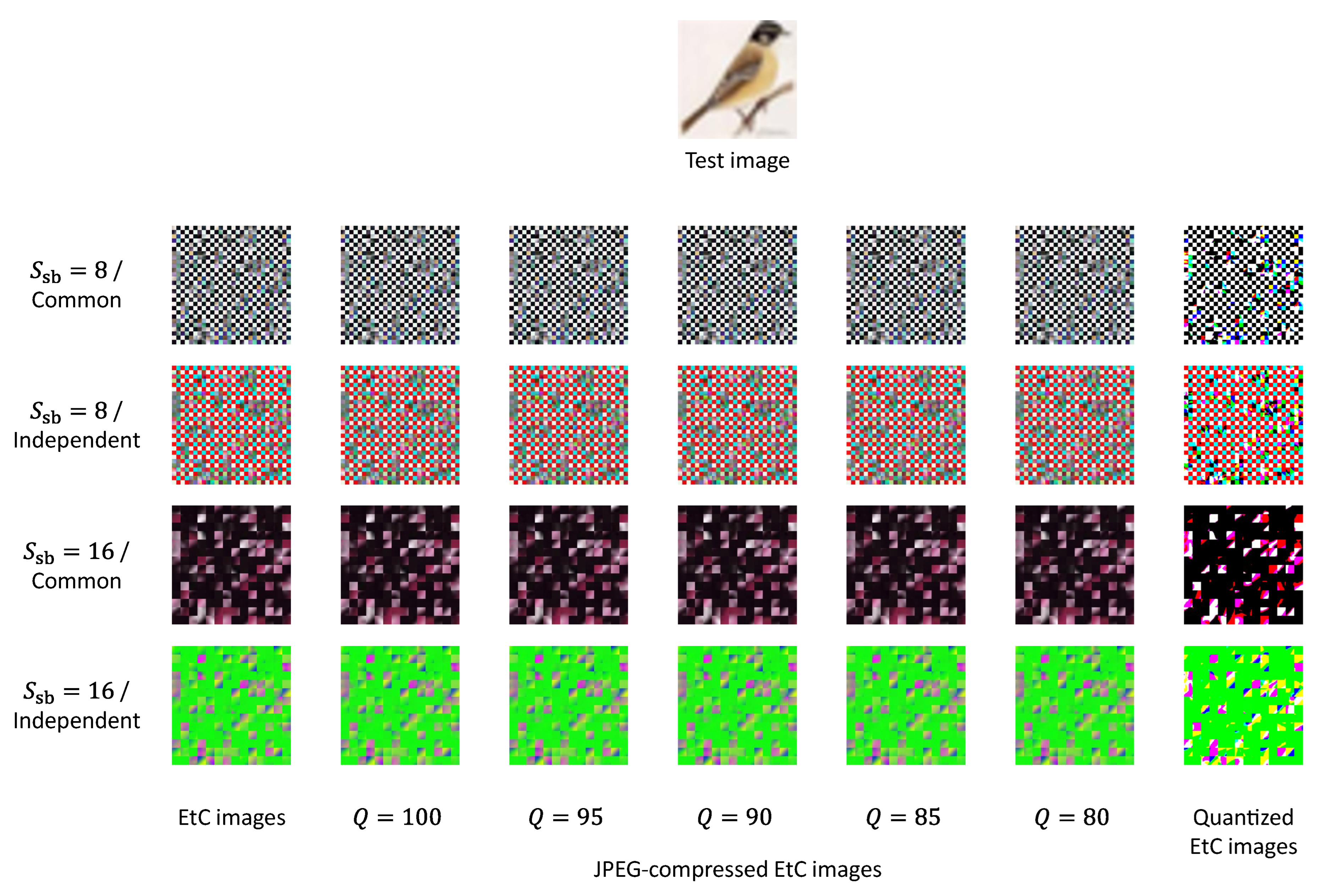
Figure 9 shows EtC, JPEG-compressed EtC and quantized EtC images for a single test image. Note that we used 4:2:0 downsampling for the JPEG compression.
4.2. Experimental Results
Table 1 shows the average amount of data in the JPEG-compressed EtC images and the quantized EtC images. This table also includes the average amount of data in the EtC images without compression and in the plain test images with and without compression. After the linear quantization, pixel values of each color component are represented by a single bit, and so the average amount of image data is 3 bpp. This table indicates that JPEG compression with
reduced a larger amount of data than linear quantization. We also found that the JPEG-compressed EtC images with
and common transformation had an analogous amount of data to the plain test images with JPEG compression at each value of
Q.
Table 2 summarizes the classification accuracy and change rate for scheme A. For comparison, this table also gives the results for the quantized EtC images through the encrypted model and for the EtC images without compression through the encrypted model. Note that the latter results could be obtained by our previous method [
17]. This table also provides the results for the plain test images with and without compression through the plain model. The change rate is calculated on the basis of the classification results for the plain test images without compression through the plain model.
With each value of Q, the classification accuracy and change rate for any encryption pattern were nearly equal to those obtained by using the plain test images and model. It is also clear that JPEG compression for the EtC images preserved a significantly high classification accuracy with a low change rate in any case, while the linear quantization sacrificed the accuracy in return for data reduction. For scheme A, the lowest classification accuracy and highest change rate were obtained in the case of , , and independent transformation. Even with this pattern, the classification accuracy was still 97.67%, and the change rate was still low at 1.94%.
Table 3 shows the classification accuracy for scheme B with
. Here, the model was trained with JPEG training images. In this table, we include the results for the plain test images with JPEG compression through the plain model. For further comparison, this table also includes the results obtained by using linear quantization. In this case, the model was trained with quantized training images. As shown in this table, JPEG compression for both the training images and the EtC images hardly degraded the classification accuracy, while the linear quantization still substantially decreased the accuracy.
Comparing scheme B and scheme A with
in
Table 2, the classification accuracy for the JPEG-compressed EtC images was slightly improved by using the encrypted model trained with the JPEG training images. Accordingly, the results for schemes A and B show that JPEG compression for training images was comparatively effective in improving the classification accuracy for JPEG-compressed EtC images.
4.3. Discussion
Here, we discuss the effects of JPEG compression for EtC images.
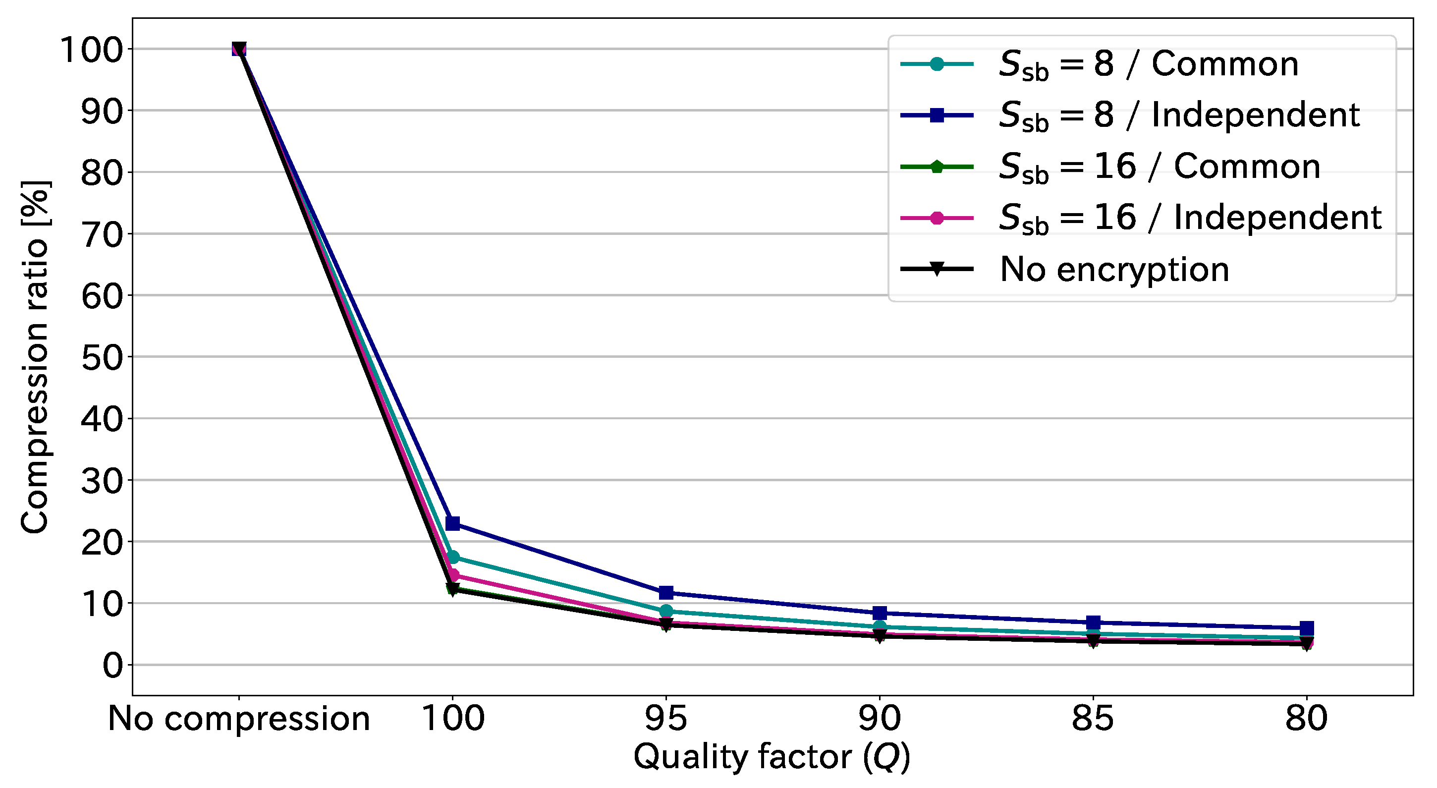
Figure 10 illustrates the compression ratio at each quality factor. This figure is derived from the results in
Table 1. The compression ratio is given by
Note that the amount of uncompressed EtC-image data is constantly 24.00 bpp. As shown in
Figure 10, the non-encrypted images, i.e., original images, had a comparable performance to the EtC images with
and common transformation. This means that the suitable conditions for the EtC system do not affect the compression performance. The figure also shows that JPEG compression could reduce the data amount 75–90% at the highest quality factor,
. Further, the data amount decreased by more than 90% in the case of
. These results demonstrate that JPEG compression can significantly reduce the amount of EtC-image data.
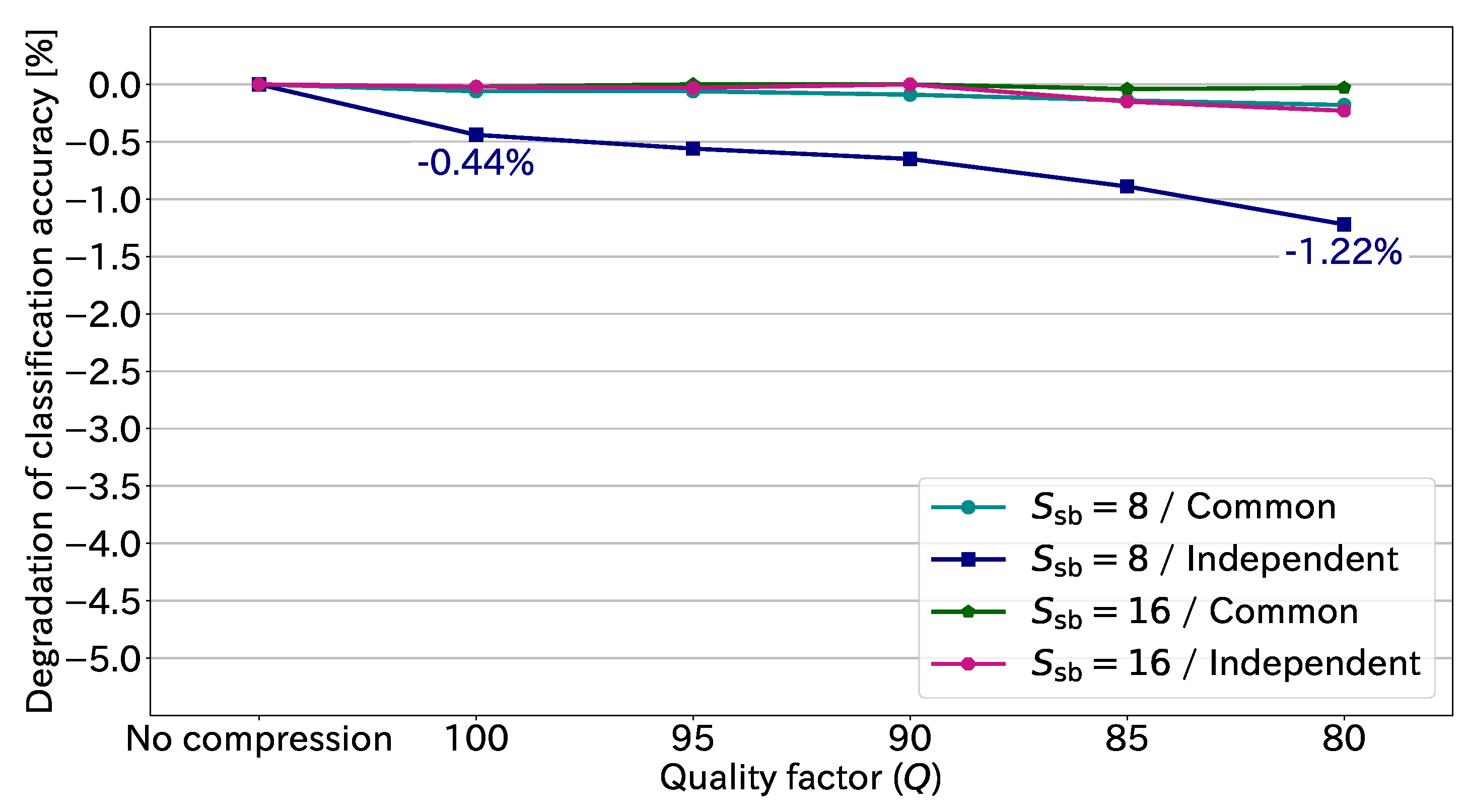
On the basis of
Table 2, we show the degradation in classification accuracy caused by JPEG compression in
Figure 11. The negative sign indicates degradation. The maximum degradation in this figure was 1.22% in the case of the independent transformation with
and
. Thus, JPEG compression in practical use causes little degradation to the classification accuracy. We can conclude that JPEG compression is effective in drastically reducing the amount of EtC-image data while preserving high classification accuracy.
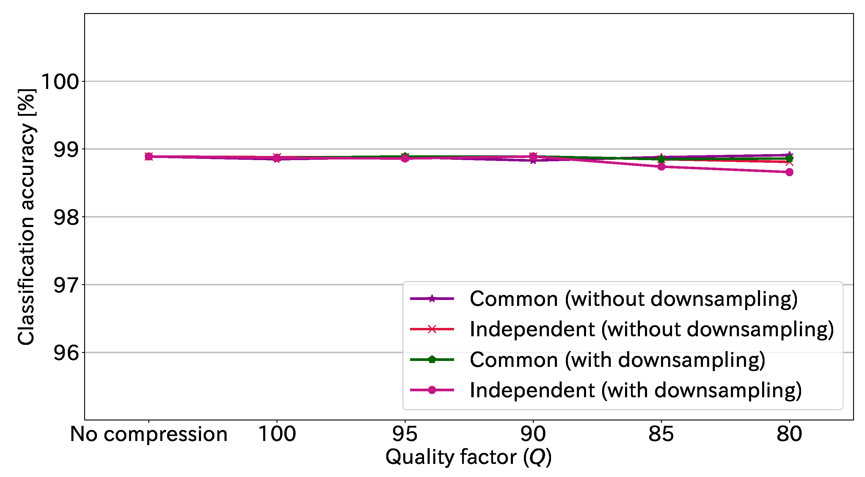
JPEG compression has an option to not downsample the chrominance component.
Figure 12 shows the classification accuracy at each quality factor with and without downsampling. Note that
is 16 in this figure. We confirmed that the classification accuracies with and without downsampling had similar trends.
We employed the EtC system on the premise of applying JPEG compression. The main-block size in the EtC system was the same as the patch size in ViT. It is important that both the main-block and sub-block sizes are multiples of 8 (or 16 with downsampling) to be equal to the block size of JPEG. Therefore, the main-block and sub-block sizes should be defined on the basis of the block size of JPEG. When the block-size condition is not satisfied, we confirmed that the classification accuracy and compression performance degraded significantly. In other words, the condition allows us to keep the classification accuracy and compression performance high.
JPEG compression generally eliminates image data in the high-frequency component. Therefore, this study suggests that noise added to the high-frequency component has little effect on ViT classification. Additionally, noise-added encrypted images generally have high robustness against attacks. Thus, JPEG noise is also expected to enhance the robustness of EtC images against attacks.


