Time Difference of Arrival (TDOA) is a technique used to determine the location of a transmitter by measuring the time difference of arrival (TDOA) of a signal at multiple receivers. TDOA location estimation is based on the principle that the signal from the transmitter will arrive at each receiver at a slightly different time due to the distance between the transmitter and the receivers. By measuring the time difference of arrival of the signal at each receiver, it is possible to determine the transmitter’s location. TDOA location estimation can be performed using either a time-based or frequency-based approach. In a time-based approach, the time difference of arrival is directly measured by comparing the signal arrival times at each receiver. This can be done using high-precision clocks to measure the arrival time of the signal at each receiver. In a frequency-based approach, the frequency difference of arrival is measured and used to calculate the time difference of arrival. This can be done by measuring the frequency shift of the signal due to the Doppler effect caused by the relative motion between the transmitter and the receivers. TDOA location estimation can also be performed using either a single-tone or a multi-tone approach. In a single-tone approach, a single frequency is used for the transmitted signal, while in a multi-tone approach, multiple frequencies are used. The use of multiple frequencies allows for the use of frequency-based TDOA estimation, which can be more accurate than time-based TDOA estimation in certain situations.
One of the challenges in TDOA location estimation is the need to accurately synchronize the clocks of the receivers, as even small clock errors can significantly impact the accuracy of the TDOA measurements. To mitigate the impact of clock errors, TDOA location estimation can be performed using a network of receivers rather than a single receiver, which allows for calculating clock error compensation values.
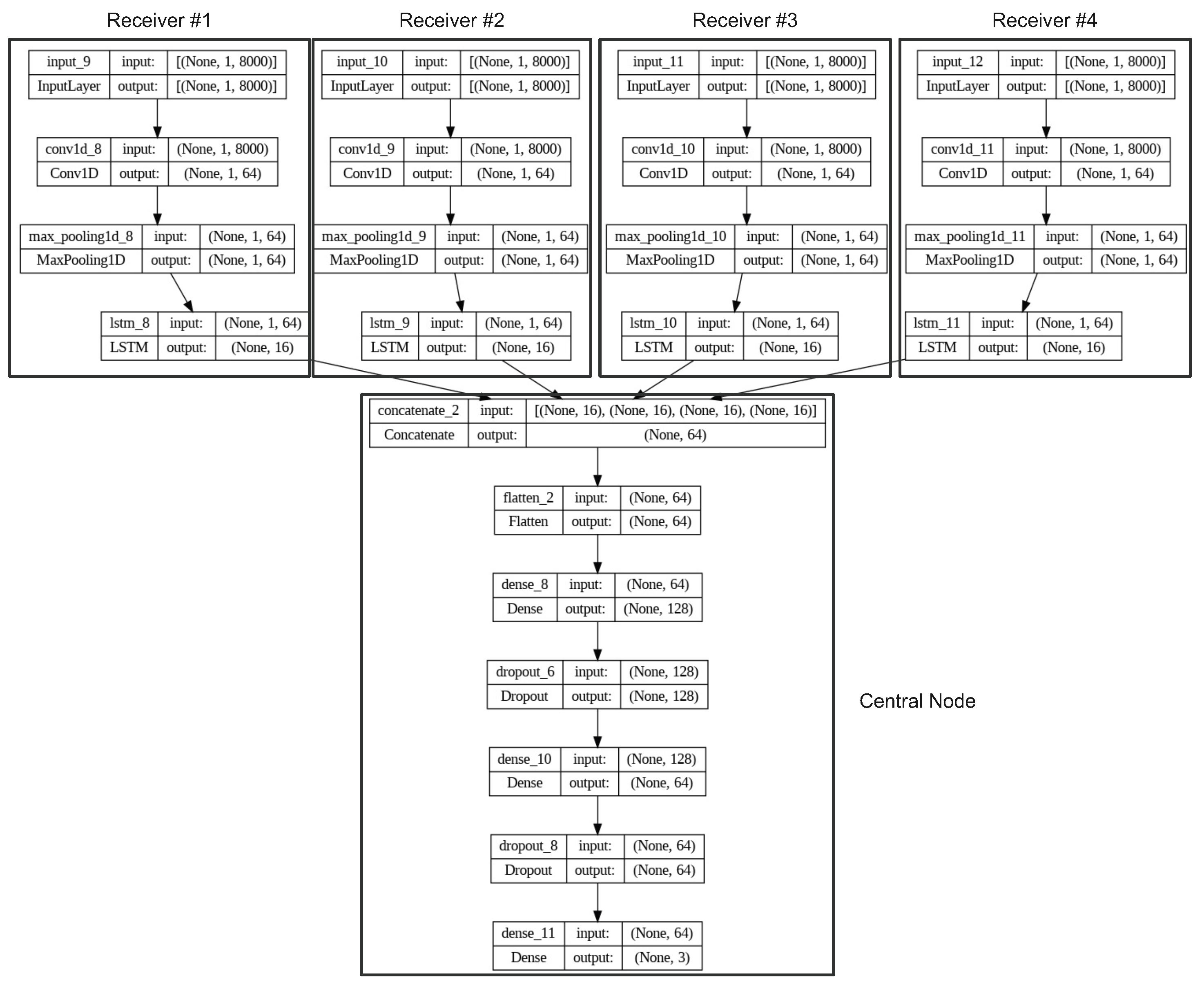
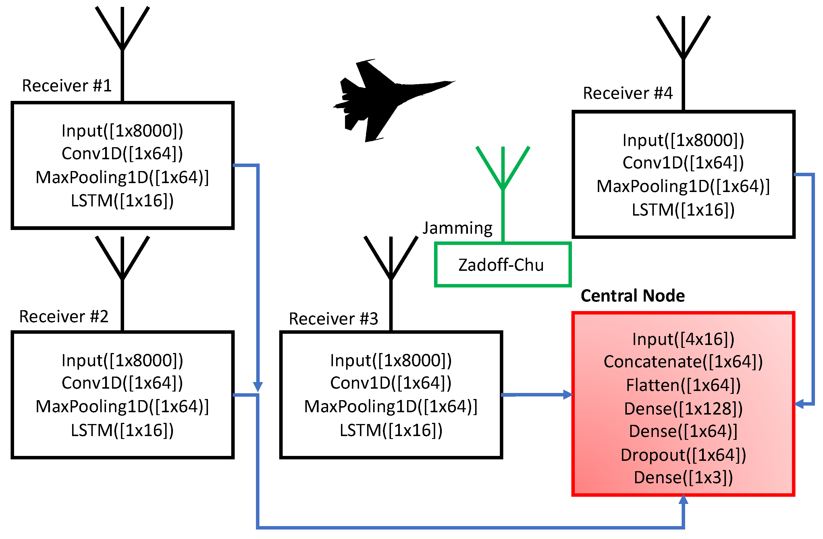
A key challenge with contemporary radar systems is their requirement for high spatial resolution, which necessitates the use of wide-band sampling. However, the transfer of sampled signals to a central processing node can be an arduous and demanding task. While optical links can be utilized to aggregate several receiving nodes, such an approach is often impractical. To address this issue, this paper presents a novel method that employs a deep neural network to compress the sampled signal into a latent space, which can then be transferred to a central processing node for data processing, where the signal is expanded and analyzed.
Furthermore, the incorporation of convolution layers in the neural network enables the system to be robust against jamming. This approach is explored in the subsequent sections of this paper and evaluated using the constructed simulator.
1.1. State-of-the-Art
Overall, TDOA location estimation is a powerful tool for determining the location of a transmitter in a wireless communication system, with applications in a wide range of fields, including military and defense, transportation, and emergency response. Ongoing research in TDOA location estimation aims to improve accuracy, reliability, and efficiency, as well as to explore new applications and integration with other technologies.
TDOA location estimation can be traced back to the early 20th century with the development of the hyperbolic positioning system by Marconi and Braun in 1903. In the 1950s, the development of radar systems led to the use of TDOA for target tracking and location estimation [
3]. In the 1970s, the advent of cellular communication systems led to the development of TDOA-based location estimation techniques for mobile phone systems. In the 1980s, the Global Positioning System (GPS) was developed, which used a combination of TDOA and angle of arrival (AOA) measurements [
4] for satellite-based location estimation [
5]. In the 1990s, the widespread adoption of wireless networking technologies such as Wi-Fi and Bluetooth led to the development of TDOA-based location estimation techniques for these systems. In the early 21st century, the Internet of Things (IoT) and the increasing demand for location-based services led to further research and development in TDOA location estimation techniques. Some works already combined neural networks with TDOA systems, combining the outputs of all the individual NN to improve position estimate accuracy [
6].
Two techniques for three-dimensional target localization using bistatic range readings from several transmitter-receiver pairs in a passive radar system were first introduced by Malanowski and K. Kulp in 2012. The algorithms, called spherical interpolation (SI) and spherical intersection (SX), are based on methods used in TDOA systems and use closed-form equations. The paper includes a theoretical accuracy analysis of the algorithms, verified through Monte-Carlo simulations and a real-life example [
7].
In 2015 A. Noroozi and M. A. Sebt presented a closed-form weighted least squares method for determining the position of a target in a passive radar system with multiple transmitters and receivers using TDOA measurements. The method involves intersecting ellipsoids defined by bistatic range (BR) measurements from various transmitters and receivers. The localization formula is derived from minimizing the weighted equation error energy. To improve the method’s performance, the paper proposes two weighting matrices, one leading to an approximate maximum likelihood (ML) estimator and the other to a best linear unbiased estimator (BLUE). The paper includes numerical simulations to support the theoretical developments [
8].
An improved approach for localizing a moving target utilizing a noncoherent multiple-input multiple-output (MIMO) radar system with widely dispersed antennas was presented in 2016 by H. Yang and J. Chun. The method is based on the two-stage weighted least squares (2SWLS) approach but only requires a single reference transmitter or receiver and can easily incorporate time-of-arrival (TOA), frequency-of-arrival (FOA), TDOA, and frequency-difference-of-arrival (FDOA) data. The authors also introduce auxiliary variables to improve numerical stability and demonstrate that their method is more stable than the Group-2SWLS method while achieving the Cramer–Rao lower bound (CRLB) at higher noise levels [
9].
In 2017 A. Noroozi and M. A. Sebt presented a method for estimating the location of a single target using bistatic range measurements in a multistatic passive radar system. The proposed method uses a weighted least squares (WLS) approach to eliminate nuisance parameters, which are parameters that are unknown and cannot be estimated from the data, and to obtain an estimate of the target location. The method involves several WLS minimizations, and two different weighting matrices are derived to improve the method’s performance. One of these matrices leads to the maximum likelihood estimator (MLE), while the other leads to the best linear unbiased estimator (BLUE) [
10].
In 2020 F. Ma, F. Guo, and L. Yang addressed the problem of directly determining the positions of moving sources using the received signals. Traditional methods for localization of moving sources involve two steps. To identify the location of the moving sources, estimations of the intermediate TDOA and FDOA characteristics are performed. In contrast, the authors propose a new method that directly estimates the locations and velocities of moving sources from the received signals. To solve the problem of simultaneously estimating the high-dimensional unknown parameters, the authors propose a multiple particle filter-based method, in which the positions and velocities of the moving sources are updated alternately using separate local particle filters. The proposed method requires fewer particles compared to classic particle filters, and its convergence is proved both theoretically and numerically. The Cramer–Rao lower bound for the proposed moving source localization method is also developed. Simulation results show that the proposed method is computationally efficient and accurate in estimating the positions of moving sources [
11].
A method for calculating the location characteristics of a moving aerial target in an Internet of Vehicles (IoV) system employing space-air-ground-integrated networks was proposed by Liu et al. in 2022. (SAGINs) [
12]. The proposed method uses multiple satellites to estimate the TDOA and FDOA signals received from the moving aerial target. The distance between the target and the receiver, as well as the velocity of the moving aerial target, are then estimated using the TDOA and FDOA estimates. To suppress direct-path and multipath interference in the received signals, the authors first filter the direct wave signals in the reference channels using a band-pass filter and then apply a sequence cancellation algorithm. The time and frequency differences of arrival are then estimated using the fourth-order cyclic cumulant cross ambiguity function (FOCCCAF) of the signals in the reference channels and the four-weighted fractional Fourier transform FOCCCAF (FWFRFT-FOCCCAF) of the signals in the surveillance channels. The Cramer–Rao lower bounds of the proposed location parameter estimators are also derived to benchmark the performance of the estimators. Simulation results show that the proposed method can effectively and accurately estimate the location parameters of the moving aerial target [
12].
In recent years, advances in signal processing algorithms and machine learning techniques have led to improved accuracy and efficiency in TDOA location estimation. TDOA location estimation has also been integrated with other location estimation techniques, such as angle of arrival (AOA) and signal strength (RSS) measurements, to improve accuracy and reliability [
13,
14,
15].
TDOA location estimation is now used in a wide range of applications, including military and defense, transportation, emergency response, and the development of advanced technologies such as autonomous vehicles and smart cities. In the future, TDOA location estimation is expected to play a key role in developing intelligent transportation systems and advancing communication technologies such as 5G and beyond. Ongoing research in TDOA location estimation aims to improve accuracy, reliability, and efficiency, as well as to explore new applications and integration with other technologies. Some of the current areas of research in TDOA location estimation include the development of advanced signal processing algorithms, the use of machine learning techniques, and the integration of TDOA with other location estimation techniques such as AOA and RSS measurements.
Passive electronic support measurement tracker (PET) systems are also known as passive surveillance systems (PSS), and their principles and technology are highly similar to radar technology from a passive radar point of view [
16]. Many PET systems are based on the multilateration TDOA method to determine the exact position of targets and can ordinarily track them. The target for this article means an emitter, which is placed on a moving platform and emits electromagnetic signals such as radar, radios, etc. PET TDOA systems are mostly dedicated to land, air, sea, and space situational awareness (SA) in military or non-military purposes such as air traffic control (ATC) and other uses [
17,
18]. In the case of SA ATC, the PET TDOA system utilizes a secondary surveillance radar aircraft transponder’s reply signals to locate, identify, and track aircraft in the large area [
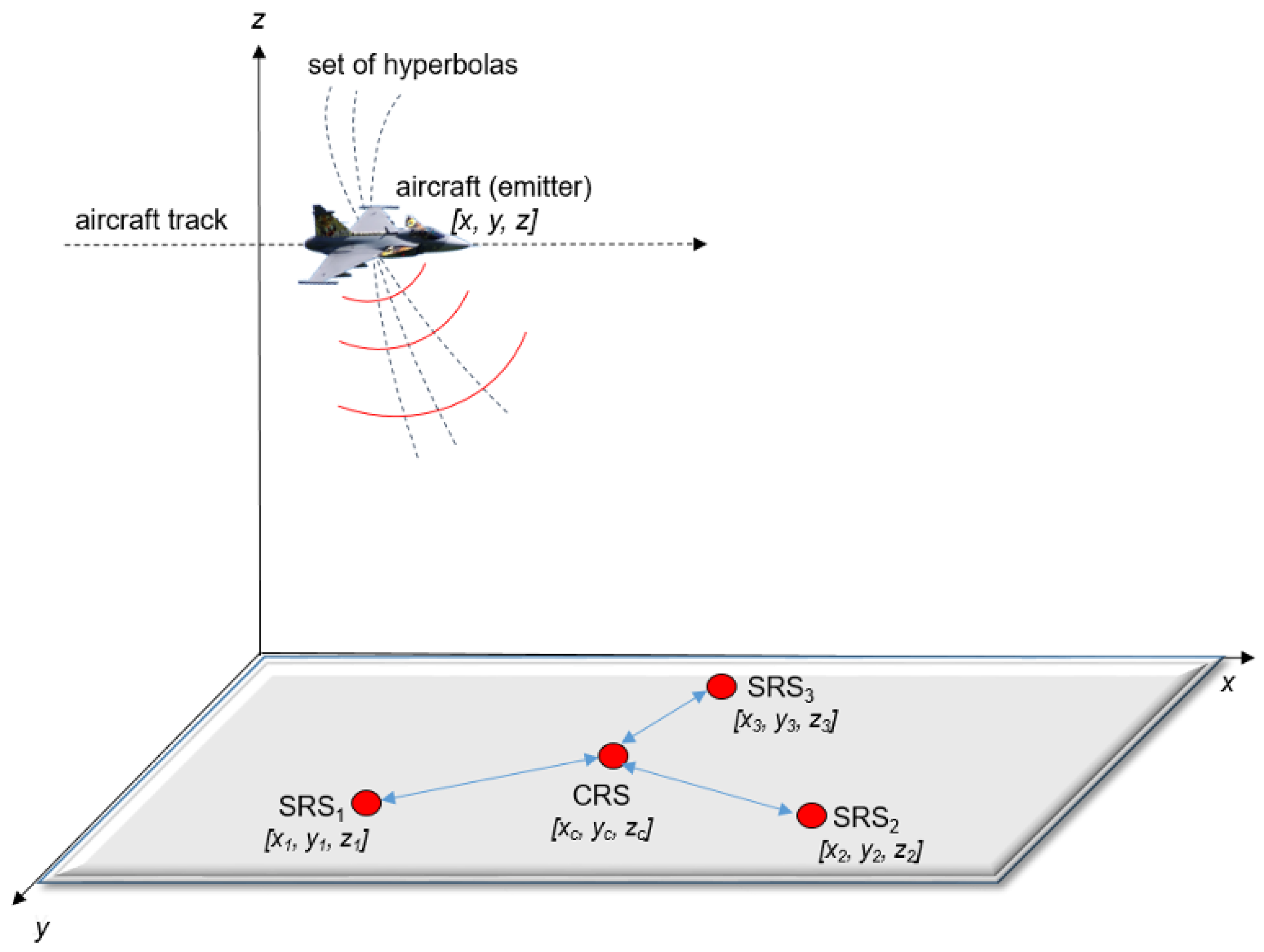
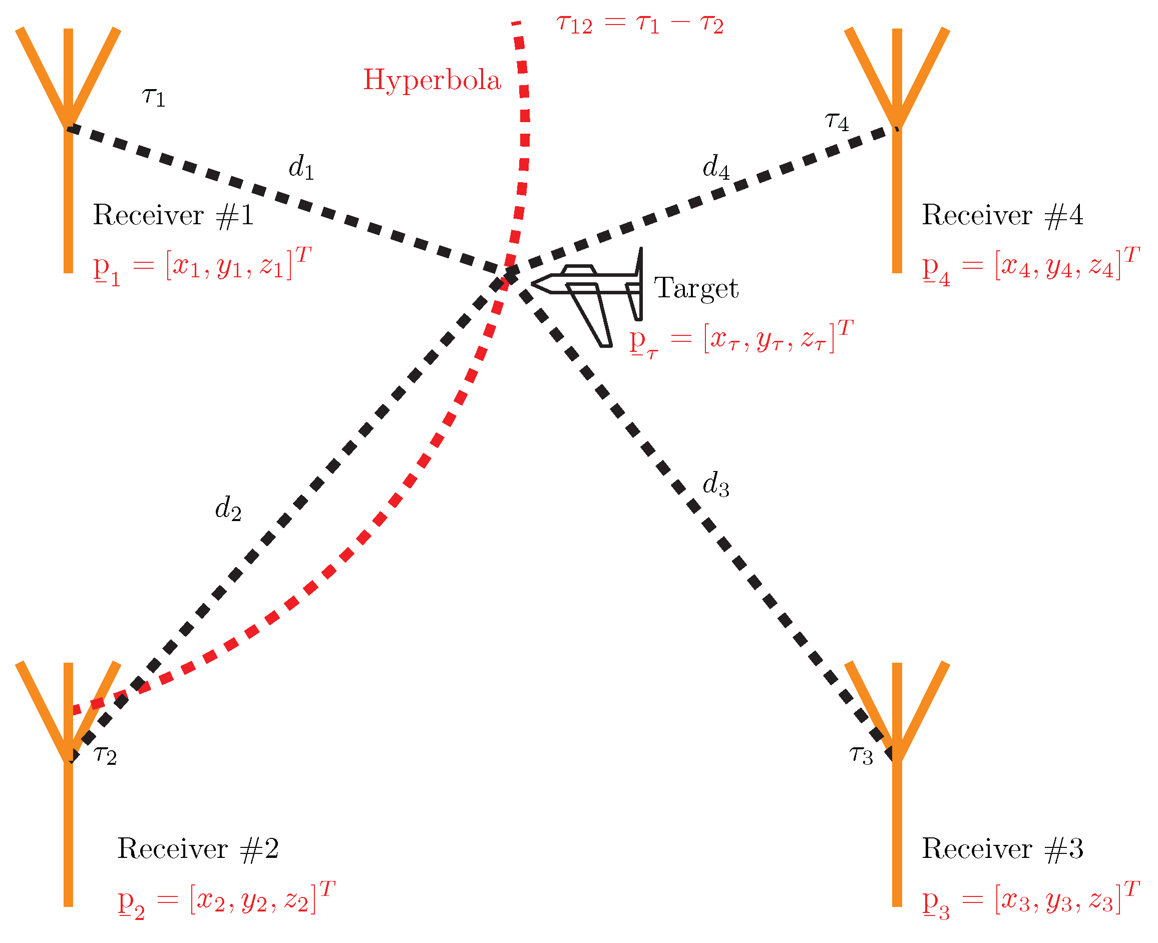
17]. If a 3D target position is required, a PET TDOA consists of four receiving stations, such as the central receiving station (CRS) and three side receiving stations (SRS1, SRS2, SRS3), see
Figure 1.
All receiving stations are placed in terrain with radio visibility towards the target, and the exact coordinates
of CRS, SRS1, SRS2, and SRS3 are known. All signals emitting from the target received by CRS, SRS1, SRS2, and SRS3 are led to the signal processing where the TDOA method is applied [
17,
18]. The TDOA method relies on the knowledge of the receiver’s coordinates and the time of signal arrival at each receiving station to compute the hyperbolic coordinates of the emitter. CRS is considered a reference. The general configuration of the four-position PET TDOA system is shown in
Figure 1. This TDOA measurement between CRS and SRS1 establishes an isodelay (hyperbolic) curve that passes through the emitter (target) location. The second hyperbola is calculated between CRS and SRS2, and the last is established between CRS and SRS3. The intersection of the set of hyperbolas locates the emitter, as shown in
Figure 1.
1.2. Neural Networks
A neural network is a type of artificial intelligence system that is inspired by the structure and function of the human brain. An input layer, one or more hidden layers, and an output layer are only a few of the layers of interconnected neurons or nodes that make up this system. Numerous tasks, including as classification, regression, and function approximation, are carried out using neural networks. They are particularly well-suited for tasks where the input and output are fixed-length, and the relationships between them are well-defined [
19].
Neural networks are trained using an optimization algorithm, such as stochastic gradient descent (SGD), which adjusts the weights and biases of the network to minimize the error between the predicted output and the true output. This process is known as backpropagation, which involves propagating the error back through the network and updating the weights and biases in each layer [
19].
The capacity of neural networks to learn from and adjust to incoming data is one of its main advantages. They can learn complex relationships between the input and output data and generalize to new data, making them effective at tasks such as image classification and speech recognition [
19].
Despite their success, neural networks do have some limitations. They can be sensitive to the quality and scale of the input data and may require preprocessing or data augmentation to achieve good results. In addition, neural networks can be computationally expensive to train, requiring specialized hardware and optimization techniques to achieve good performance [
19].
Feed-forward neural networks, recurrent neural networks, and convolutional neural networks are a few of the several types of neural networks. Each type is designed for specific types of tasks and data, and selecting the appropriate type of neural network for a given task is an important consideration in the design and implementation of an AI system [
19].
In this research, we suggest combining several neural networks. Since neural networks are nowadays penetrating all fields of science, we wondered if they could have a benefit in TDOA systems. Therefore, in the following paragraphs, we describe in general terms the different neural networks we have used in the design of the network architecture [
19].
1.2.1. Perceptron
One layer of neurons or nodes makes up a perceptron, an artificial neural network. Frank Rosenblatt developed it in the 1950s as a way to simulate the learning process of the human brain. Perceptrons are used for various tasks, including classification, regression, and function approximation. They are particularly well-suited for tasks where the input and output are fixed-length, and the relationships between them are well-defined [
19].
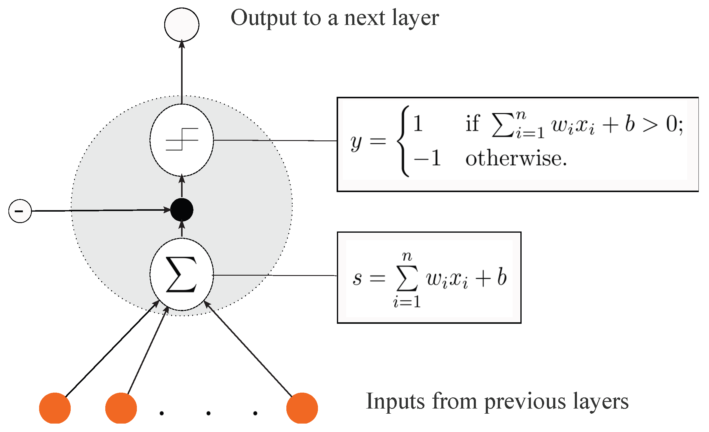
The structure of a perceptron consists of an input layer and an output layer, with the input layer receiving the raw input data and the output layer producing the final prediction or output. The input layer is connected to the output layer through weights and biases, which are adjusted during the training process to minimize the error between the predicted output and the true output [
20].
One of the key advantages of perceptrons is their simplicity and ease of implementation. They are relatively easy to train and can be implemented using a variety of programming languages and libraries. In addition, perceptrons can be highly efficient, especially with hardware acceleration, such as graphics processing units (GPUs). In addition, perceptrons are limited in their ability to model complex relationships between the input and output data. They are only able to learn linear decision boundaries, making them less effective at tasks that require more complex decision boundaries [
20].
Given the input vector
and trained weights
, the perceptron output
y is represented by formula [
20]:
where
is the weighted input and
is the state of the perceptron. For the perceptron to be activated, the threshold value must exceed its state
s [
20]. The Boolean operations AND, OR, NAND, and NOR are just a few that the perceptron may express.
Figure 2 depicts the perceptron’s general structure [
20].
1.2.2. Feed Forward Networks
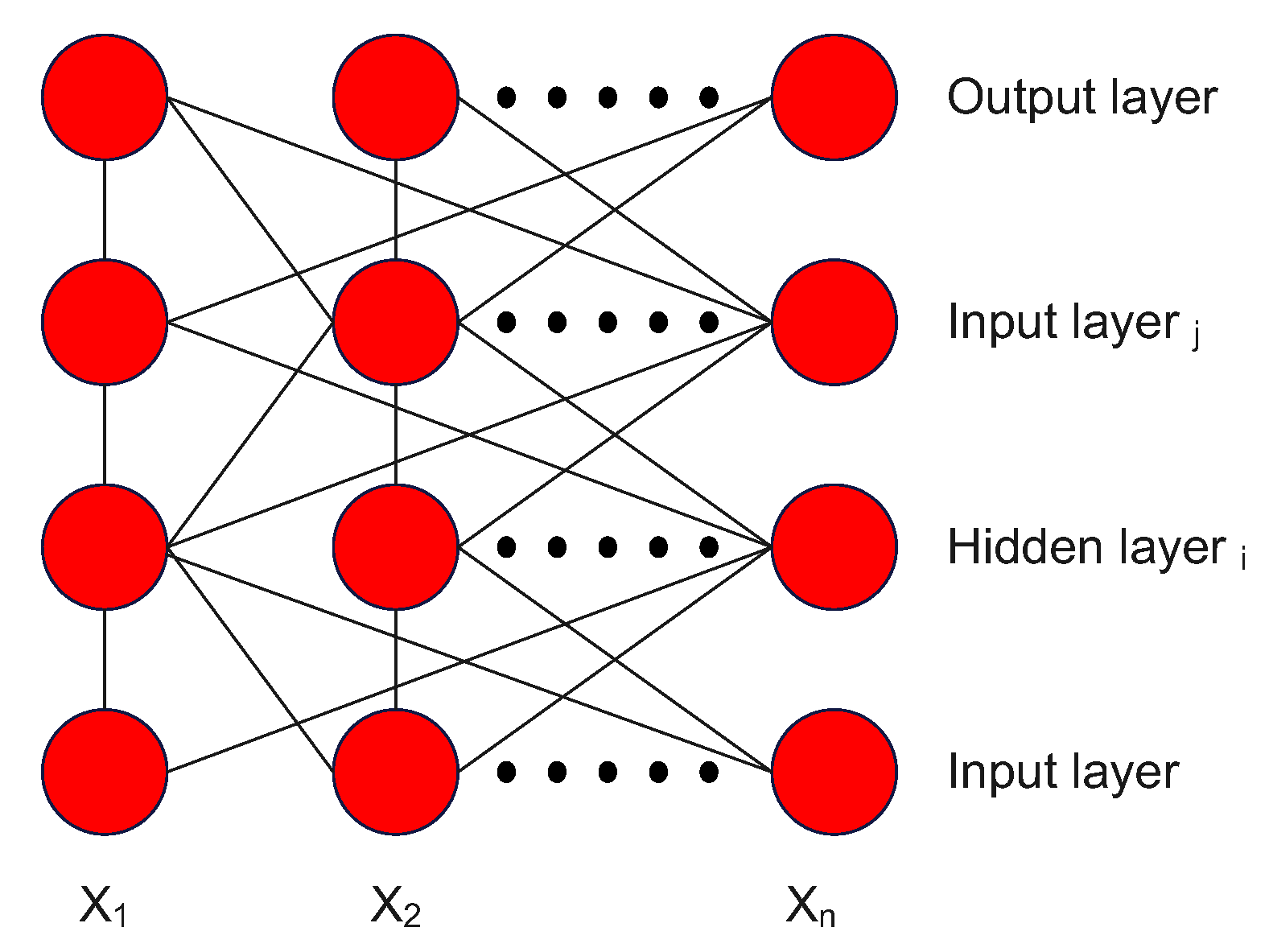
A feed-forward neural network, also known as a feed-forward network or a feed-forward artificial neural network, is a type of artificial neural network that consists of layers of interconnected neurons or nodes. It is called "feed-forward" because the information flows through the network in one direction, from the input layer to the output layer, without looping back. Feed-forward networks are used for various tasks, including classification, regression, and function approximation. They are particularly well-suited for tasks where the input and output are fixed-length, and the relationships between them are well-defined. The number of layers and neurons in each layer determines the structure of a feed-forward network. The input layer receives the raw input data, while the output layer produces the final prediction or output. The layers in between are called hidden layers, and the neurons in these layers are responsible for learning and extracting features from the input data. The main functionality of the feed-forward network is to approximate some function
. For example, we have classifier
map an input
x to a category
y. A feed-forward network defines a mapping
and learns the value of the parameters
that result in the best function approximation [
21]. The structure of layers and connections is shown in
Figure 3.
These models are called feed-forward because information flows through the function evaluated from
x, through the intermediate computations used to define
f, and finally to the output
y. There are no feedback connections in which outputs of the model are fed back into itself [
21].
A group of neurons represents the feed-forward neural network. Each of these layers of neurons compute a weighted sum of its inputs. Depending on the neuron’s location in the network, we can distinguish the basic levels of neurons. The first level is the input neurons, through which environmental signals are emitted. A group of neurons represents the feed-forward neural network. Each of these layers of neurons compute a weighted sum of its inputs. The next type is output neurons, which pass processed signals back to the environment. The last type is hidden neurons, which are inside the network and do not interact with the external environment. Feed-forward neural networks have no loops and are completely integrated. This indicates that no weights provide input to a neuron in the previous layer and that every neuron from the previous layer is connected to every neuron in the subsequent layer. Bias values are used to initialize the weights of a feed-forward neural network to small, normalized random numbers. The neural network is then trained using all training samples, and error backpropagation computes each unit’s input and output for all (hidden and visible)output layers [
20].
Feed-forward networks are trained using an optimization algorithm, such as SGD, which adjusts the weights and biases of the network to minimize the error between the predicted output and the true output. This process is known as backpropagation, which involves propagating the error back through the network and updating the weights and biases in each layer [
20].
One of the key advantages of feed-forward networks is their simplicity and ease of implementation. They are relatively easy to train and can be implemented using a variety of programming languages and libraries. In addition, feed-forward networks can be highly efficient, especially with hardware acceleration such as GPUs. Despite their simplicity, feedforward networks can be powerful tools for solving many problems. They have been used to achieve state-of-the-art performance on tasks such as image classification and speech recognition [
20].
However, feed-forward networks do have some limitations. They are not well-suited for tasks that require incorporating context or dependencies over time, such as natural language processing or speech recognition. For these tasks, recurrent neural networks (RNNs) or convolutional neural networks (CNNs) are typically used [
20].
Feed-forward neural networks are a widely used and powerful tool for solving various tasks in machine learning and artificial intelligence. They are an active area of research and will likely continue to be an important tool in developing intelligent systems.
1.2.3. Convolutional Neural Networks
Artificial neural networks known as CNNs are particularly effective at recognizing objects in images and videos. They are called “convolutional” because they use a mathematical operation called convolution to analyze the input data. This operation allows the network to learn features and patterns in the data by sliding a small matrix, called a kernel or filter, over the input and performing element-wise multiplications and summaries.
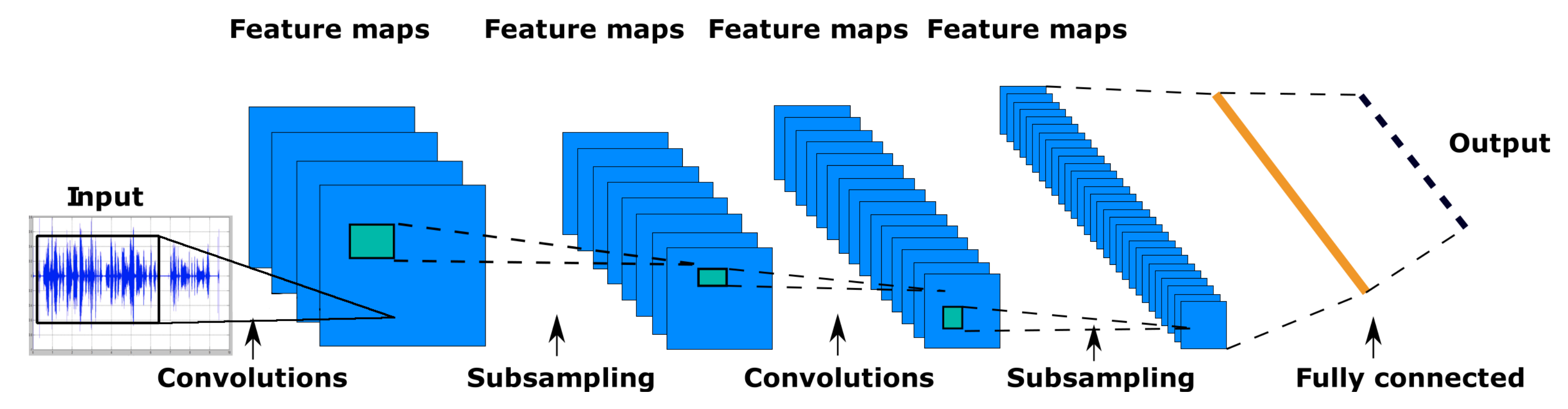
CNNs are composed of several layers of neurons, each responsible for learning a different aspect of the input data. The first layers of a CNN typically learn simple features, such as edges and corners, while the deeper layers learn more complex features, such as shapes and patterns. The output of the final layer is a prediction of the class or label of the input data. The typical architecture of CNN is shown in
Figure 4 [
22].
One of the key advantages of CNNs is their ability to learn features directly from the input data rather than requiring manual feature engineering. This allows them to achieve high performance on tasks such as image classification and object detection. In addition, CNNs can use their learned features to generalize to new data, making them effective for tasks such as image synthesis and style transfer [
22].
Despite their success, CNNs do have some limitations. They can be sensitive to the quality and scale of the input data and may require preprocessing or data augmentation to achieve good performance. In addition, CNNs can be computationally expensive to train, requiring specialized hardware and optimization techniques to achieve good performance [
22].
CNNs are widely utilized in applications including computer vision, natural language processing, and speech recognition, because they have consistently shown to be effective tools for image and video recognition tasks [
22].
CNNs are feed-forward neural networks with modified architecture. The architecture of CNNs usually consists of convolutional layers followed by a pooling layer, where each neuron in a convolutional layer is connected to some region in the input. This region is usually called a local receptive field. All weights (filters) in CNNs are shared based on the position within a receptive field. The convolution operation can be described as follows [
22]:
where
is the input image at position
and
is a trainable filter. The pooling layers in CNN reduce the dimensionality of features, which leads to a reduction of connection between the layers. Hence it reduces the computational time [
23]. In our particular case, we used autoencoders that consist of convolutional layers. The autoencoders aim to reduce a large amount of data from individual antenna nodes.
1.2.4. Recurrent Neural Network
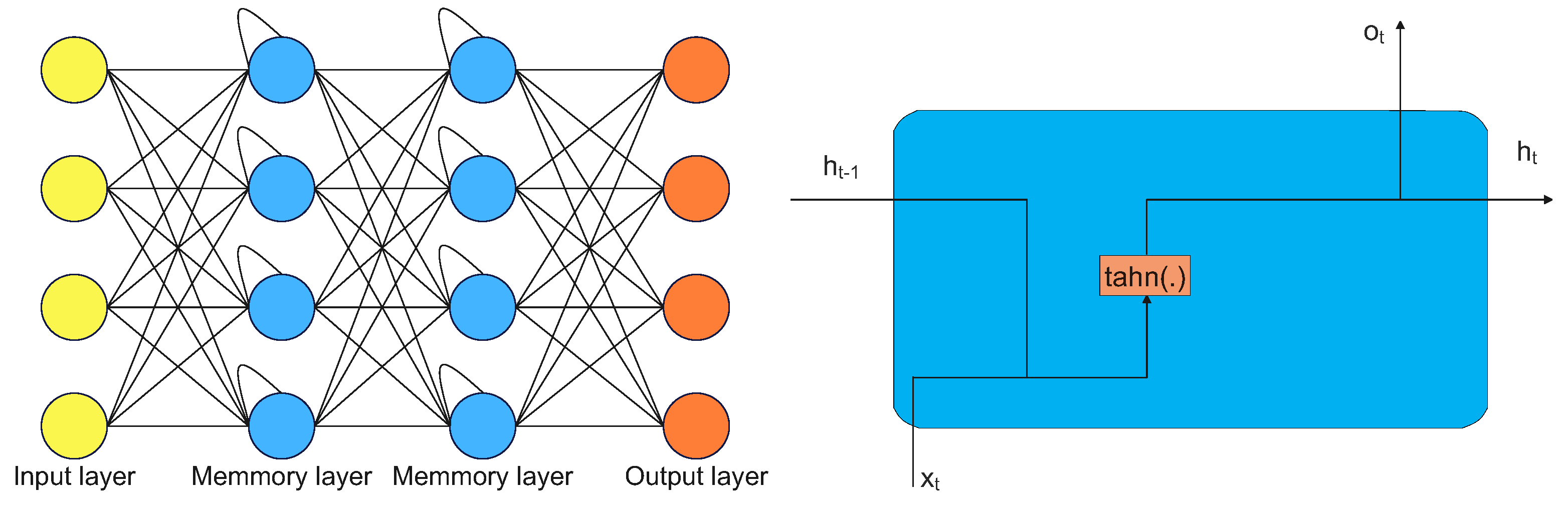
RNNs are a form of artificial neural network that excel at handling sequential input, including time series, speech, and spoken language. They are called “recurrent" because they use feedback connections, allowing the network to retain information from previous time steps and use it to inform its current output. This makes RNNs capable of learning long-term dependencies and patterns in sequential data. A typical example of RNN architecture is shown in
Figure 5 [
21].
Several RNNs, including the long short-term memory (LSTM) network and the gated recurrent unit (GRU) network are used. These architectures introduce special "memory" cells and gating mechanisms that allow the network to selectively retain and forget information as needed, helping to prevent the vanishing and exploding gradient problems that can occur in traditional RNNs. RNNs can be used for various tasks, including language translation, language modeling, machine translation, and text generation. They are also used in speech recognition, music generation, and robot controlds [
21,
24].
One of the key challenges in training RNNs is the need to process the entire input data sequence simultaneously, which can be computationally expensive. To address this issue, techniques such as truncated backpropagation through time (BPTT) and teacher forcing can reduce the sequence length that needs to be processed [
21].
Despite their success, RNNs do have some limitations. They can be difficult to train, especially for longer sequences, and may require careful optimization and regularization techniques to achieve good performance. In addition, RNNs can be sensitive to the quality and scale of the input data and may require preprocessing or data augmentation to achieve good results [
21].
One of the key advantages of RNNs is their ability to incorporate context from previous time steps into their predictions. This makes them particularly well-suited for tasks such as language translation, where the meaning of a word can depend on the words that come before and after it. Another advantage of RNNs is their ability to handle variable-length sequences. This makes them useful for tasks such as machine translation, where the length of the input and output sequences can vary greatly [
21,
24].
One of the most successful applications of RNNs is natural language processing (NLP). RNNs have been used to achieve state-of-the-art performance on tasks such as language translation, language modeling, and sentiment analysis. In addition to their success in NLP, RNNs have also been used to achieve good results in speech recognition tasks. They have been used to model the temporal dependencies in speech signals, allowing them to learn the important patterns and features for recognizing different sounds and words [
21].
Overall, recurrent neural networks are a powerful tool for processing sequential data and have found wide application in natural language processing and speech recognition tasks. Despite their challenges, they have proven to be a valuable tool for solving a wide range of problems and are an active area of research in machine learning and artificial intelligence [
21].
Typical recurrent memory architecture is shown in
Figure 5, where
represent hidden layer vectors,
is the input vector,
is the bias vector,
are the activation functions, and
are the parameter matrices. All relations are described as follows:
1.2.5. Long-Short Term Memory
LSTM is a type of RNN that is particularly well-suited for processing sequential data with long-term dependencies. Hochreiter and Schmidhuber introduced it in 1997 to solve the vanishing gradient problem that affects traditional RNNs. LSTMs are composed of special “memory” cells that can retain information for extended periods and gating mechanisms that allow the network to retain or forget information as needed selectively. The input, forget, and output gates allow the LSTM to control the flow of information into and out of the memory cells, while the cell state serves as the internal memory of the LSTM [
21].
LSTMs have been used to achieve state-of-the-art performance on tasks such as language translation, language modeling, machine translation, and speech recognition. They have proven to be particularly effective at capturing long-term dependencies in sequential data, allowing them to learn complex patterns and structures. One of the key advantages of LSTMs is their ability to handle variable-length sequences, making them useful for tasks such as machine translation, where the length of the input and output sequences can vary greatly. They can also incorporate context from previous time steps into their predictions, making them well-suited for tasks such as language translation, where the meaning of a word can depend on the words that come before and after it [
25].
Despite their success, LSTMs do have some limitations. They can be computationally expensive to train and require careful optimization and regularization techniques to achieve good performance. In addition, LSTMs can be sensitive to the quality and scale of the input data and may require preprocessing or data augmentation to achieve good results [
25].
One area of active research in the field of LSTMs is the development of more efficient architectures and training techniques. This includes using techniques such as weight tying and pruning to reduce the number of parameters in the network, as well as using optimization algorithms such as Adam and SGD with momentum to speed up training [
25].
Another area of research is the development of LSTM variants that are better suited for specific tasks or types of data. For example, attention mechanisms have been introduced to allow LSTMs to focus on specific parts of the input sequence when making predictions [
25].
Overall, LSTMs have proven to be a powerful tool for processing sequential data and have found wide application in natural language processing and speech recognition tasks. They are an active area of research in machine learning and artificial intelligence. They will likely continue to be an important tool in developing intelligent systems [
25].
Each memory block in the original architecture contained an input and output gate. The input gate controls the flow of input activations into the memory cell. The output gate controls the output flow of cell activations into the rest of the network. Later, the forget gate was added to the memory block [
25].
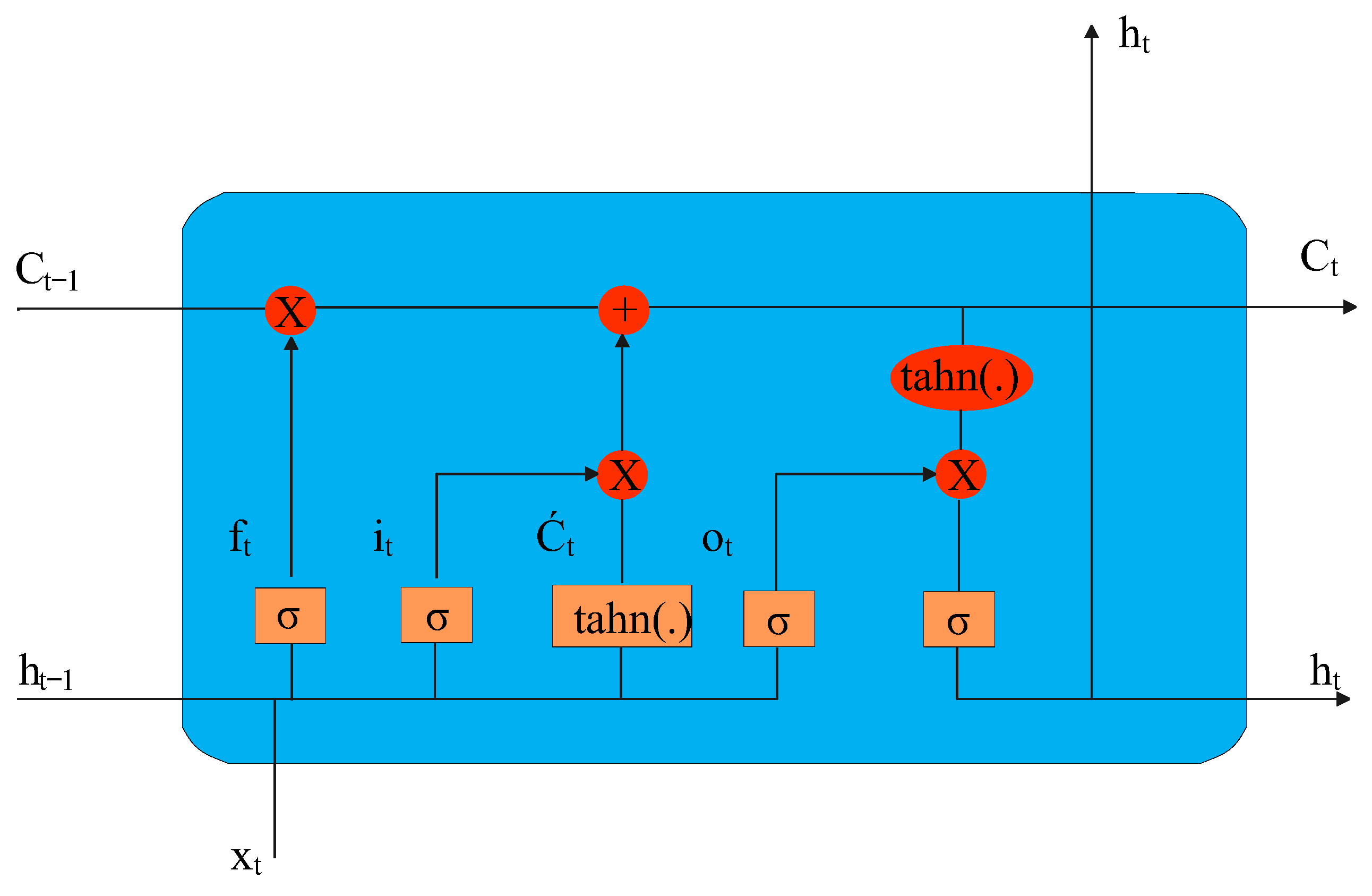
A typical LSTM architecture is shown in
Figure 6, where
represents the hidden layer vectors,
is the input vector,
are the bias vectors, and
tanh are the activation functions. Functions
are described as follows:
1.2.6. Gated Recurrent Unit
A particular kind of RNN that excels at processing sequential data with long-term dependencies is the gated recurrent unit (GRU). It was introduced by Cho et al. in 2014 as a simplified version of the LSTM network, which was developed to address the vanishing gradient problem that affects traditional RNNs. GRUs are composed of special "memory" cells and gating mechanisms that allow the network to selectively retain or forget information as needed. The update and reset gates control the flow of information into and out of the memory cells, while the cell state serves as the internal memory of the GRU [
25].
Micro-Doppler Effect and Determination of Rotor Blades by Deep Neural Networks Speech recognition, language modeling, machine translation, and other activities have all benefited from the employment of GRUs. They have proven particularly effective at capturing long-term dependencies in sequential data, allowing them to learn complex patterns and structures. One of the key advantages of GRUs is their simplicity and efficiency compared to LSTMs. They have fewer parameters and require less computation, making them faster to train and easier to optimize. They can also handle variable-length sequences, making them useful for tasks such as machine translation, where the length of the input and output sequences can vary greatly [
25].
Despite their success, GRUs does have some limitations. They may not be as powerful as LSTMs on certain tasks, especially those that require more complex memory mechanisms. In addition, GRUs can be sensitive to the quality and scale of the input data and may require preprocessing or data augmentation to achieve good results [
25].
One area of active research in the field of GRUs is the development of more efficient training techniques. This includes using techniques such as weight tying and pruning to reduce the number of parameters in the network, as well as using optimization algorithms such as Adam and SGD with momentum to speed up training. Another area of research is the development of GRU variants better suited for specific tasks or data types. For example, attention mechanisms have been introduced to allow GRUs to focus on specific parts of the input sequence when making predictions [
25].
GRUs have proven to be a useful tool for processing sequential data and have found wide application in natural language processing and speech recognition tasks. They are an active area of research in machine learning and artificial intelligence and will likely continue to be an important tool in developing intelligent systems [
25].
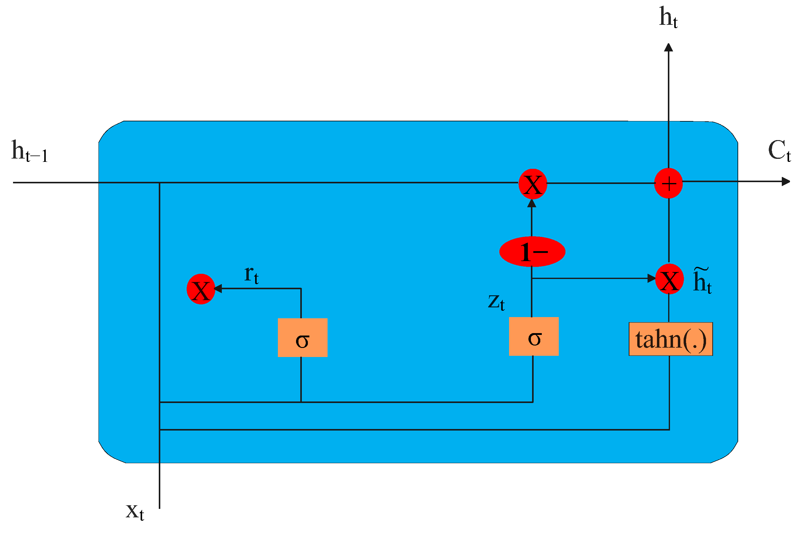
The typical LSTM architecture is shown in
Figure 7, where
represents hidden layer vectors,
is the input vector,
are the bias vectors,
are the parameter matrices, and
tanh are the activation functions. Functions
are described as follows:
1.3. TDOA Detection Methods
TDOA is a technique used to determine the location of a radio transmitter based on the difference in the time it takes a radio signal to reach different receivers. It works by measuring the time difference between when a signal is received at two or more different locations and then using that information to triangulate the transmitter’s position. TDOA is based on the principle that the speed of light c is constant and that the time it takes for a radio signal to travel from the transmitter to each receiver can be accurately measured. This method can be used for both passive and active location systems, and it is commonly used in military and civilian applications such as wireless communication, navigation, and surveillance.
There are several advantages to using the TDOA method:
However, there are also some disadvantages to using TDOA:
Accurate and synchronized clocks are required for each sensor to ensure the accuracy of the TDOA estimation;
TDOA estimation accuracy can be affected by measurement errors on sensor positions, the multipath problem (signal reflection), the sensors’ timing accuracy, and the sensors’ geometry concerning the target.
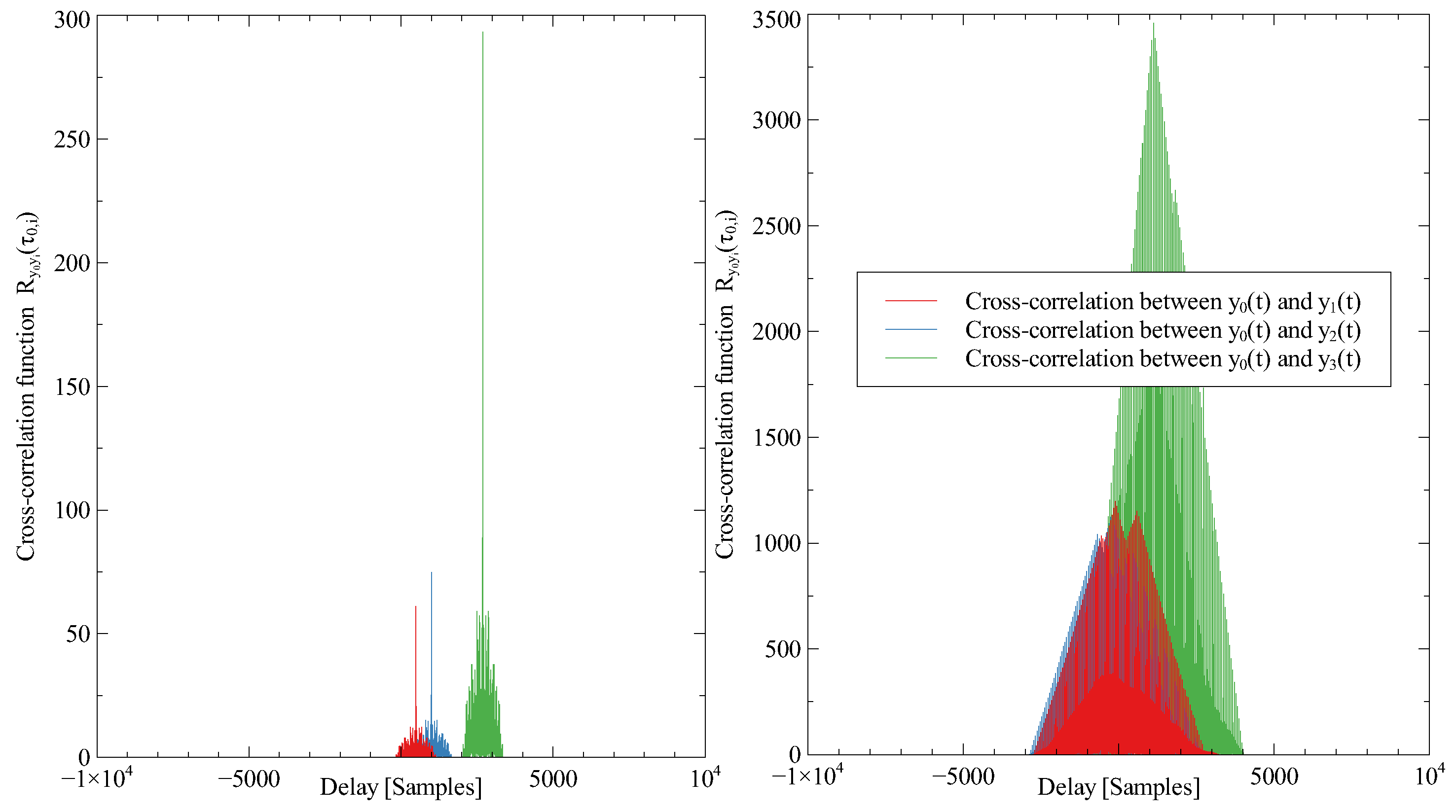
In a TDOA scenario, it is assumed that the sensors are stationary and synchronized, resulting in no Doppler shifts for any of the sensors. To estimate the TDOA, the cross-correlation between signals received by different sensors is typically calculated using a classical approach. TDOA localization scenario is shown in
Figure 8. Each sensor receives the signal with some delay in time and frequency. The received signal for
i-th sensor is shown as,
where
is the phase introduced by the time of flight of the signal and
is the Doppler frequency shift of
i-th sensor with velocity where
and
. Hence, the TDOA value between the first and second sensors can be determined by locating the peak of the cross-correlation function
Finding the peak of
gives a TDOA value between 1st and 2nd receiving antenna
, we can write
by using the distance
and
as
and using propagation speed (speed of light
. Some works have used unknown propagation speed, such as in Ref. [
27])
c as
. To generalize, we can estimate the distances for points given by Cartesian coordinates in n-dimensional Euclidean space between the antenna and target
T as the Euclidean distance:
The equation can be rewritten for clarity and emphasis as follows (using the Cartesian coordinates
:
The equation can be solved, e.g., by Taylor series expansion (using at least four sensors) or by adding a new variable and doing the linearization (at least five receiving antennas are needed). Note that time differences are not affected by errors in the receiver’s clock time as it cancels out when subtracting two measurements.
For simplicity, the task is reduced to 2D, and the position is calculated as follows [
28]:
which yields the following least-squares intermediate solution:
where
.


