
Path Planning of a Mobile Delivery Robot Operating in a Multi-Story Building Based on a Predefined Navigation Tree


Abstract
:1. Introduction
1.1. Problem Definition
1.2. Proposed Solution
- The manual definition of a navigation tree describing the spatial information required to autonomously move in a multi-story building, using the elevators as connectors between floors.
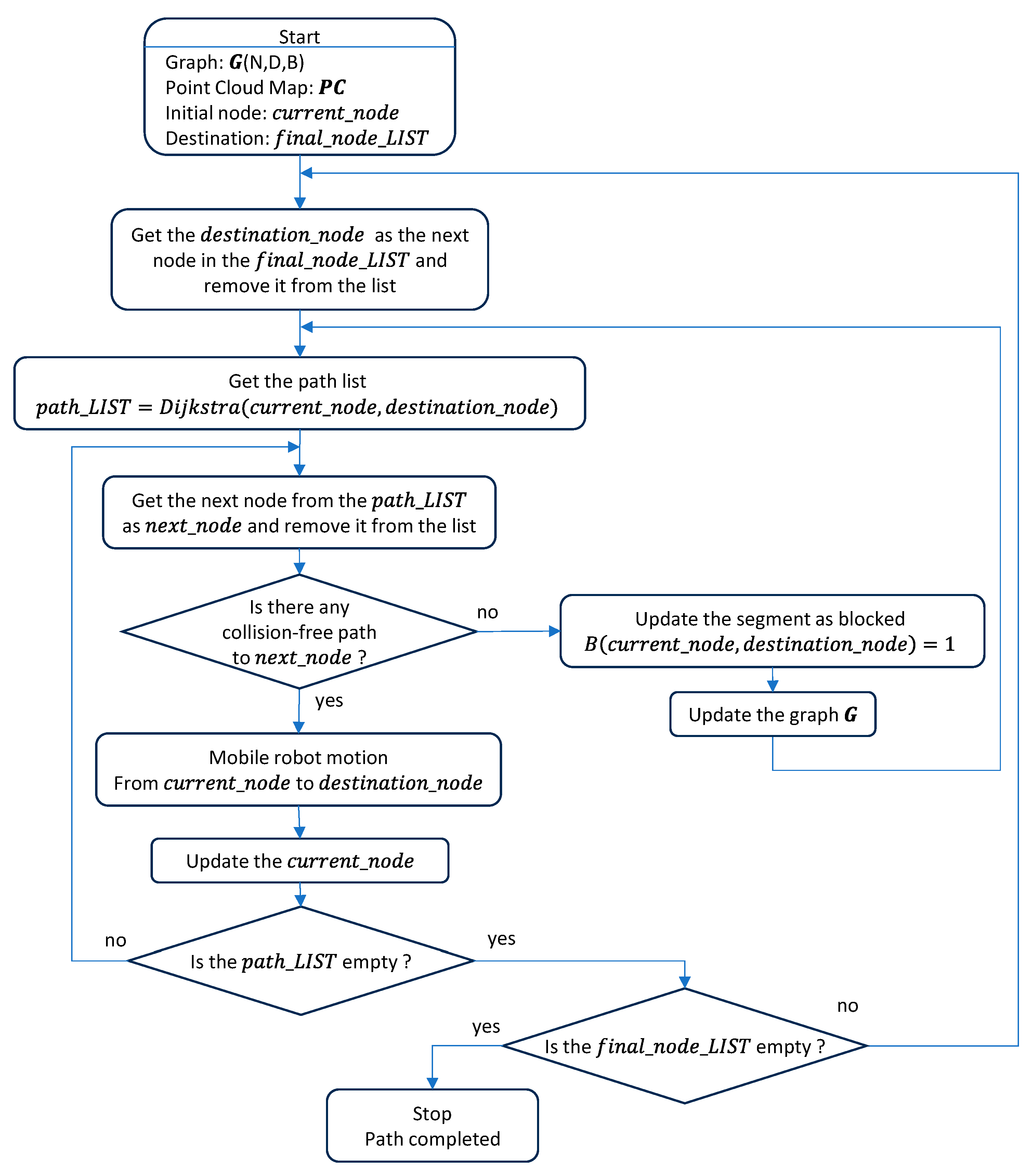
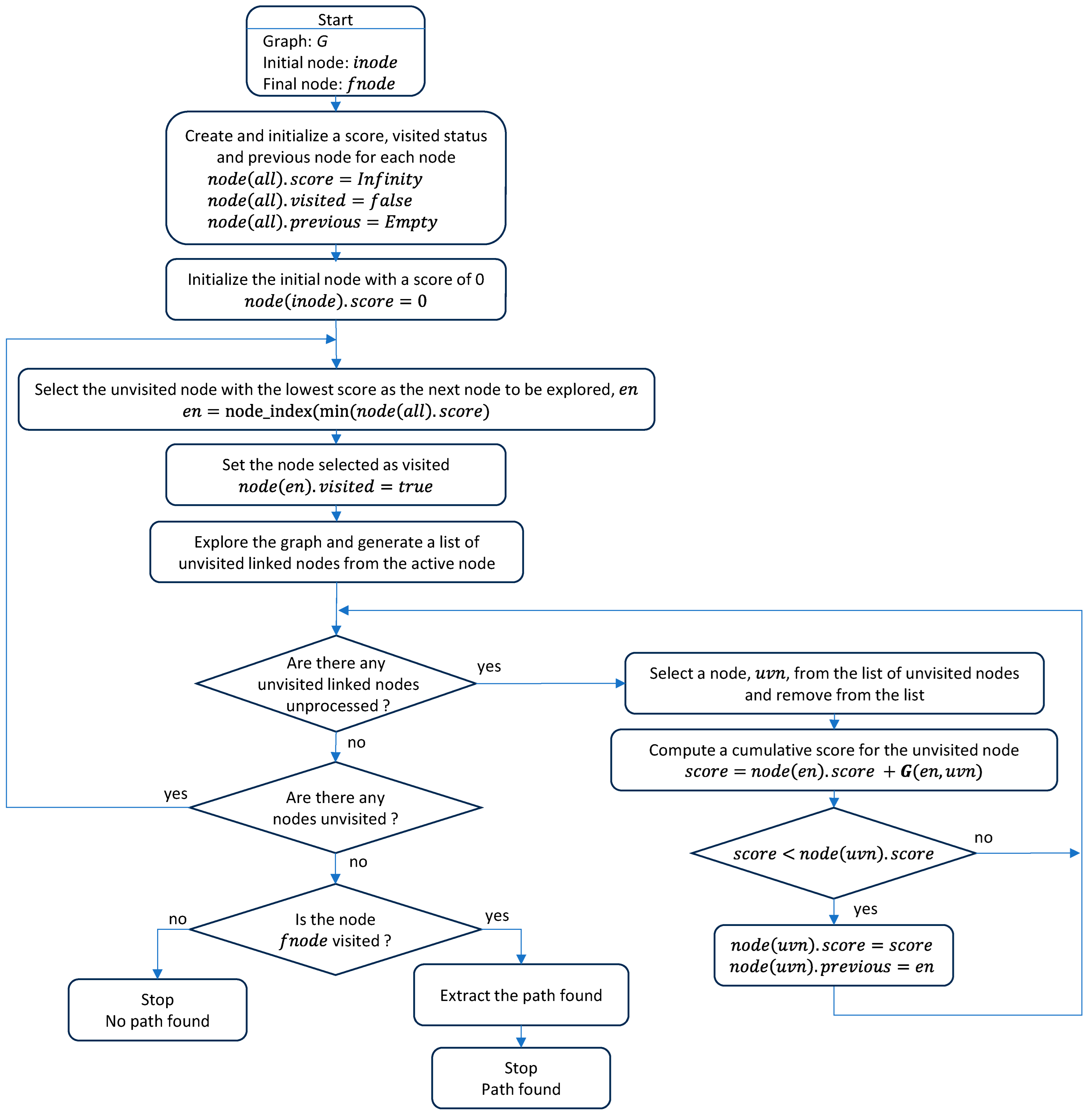
- The description of how a graph created from this navigation tree can be explored using Dijkstra’s [88] algorithm to obtain the shortest path from a starting point to a destination point.
- The formulation of a distance–task matrix that can be used to estimate the total length of the trajectory of a mobile delivery robot moving in a multi-story building.
- The presentation of simulation examples that demonstrate the effectiveness of this proposal in the case of a mobile robot designed to transport and deliver small packages in a multi-story building.
1.3. Assumptions and Limitations
- A detailed 2D point cloud map of the multi-story building is available [31].
- All locations where a package can be picked up or dropped off inside the multi-story building have been identified as nodes and do not change during transportation.
- The multi-story building has remotely controlled elevators that can be directly accessed by a mobile robot via a wireless communication protocol [30].
- A navigation tree for each floor of the building has been manually defined.
- A segment (connection, link or vertex) defined in the navigation tree depicts a straight collision-free trajectory between two nodes. This straight trajectory can be blocked by the presence of dynamic obstacles.
- Packages are only delivered to locations that have their doors open. The problem of opening and closing the doors of the rooms is not covered in this work.
1.4. Structure of the Paper
2. Materials and Methods
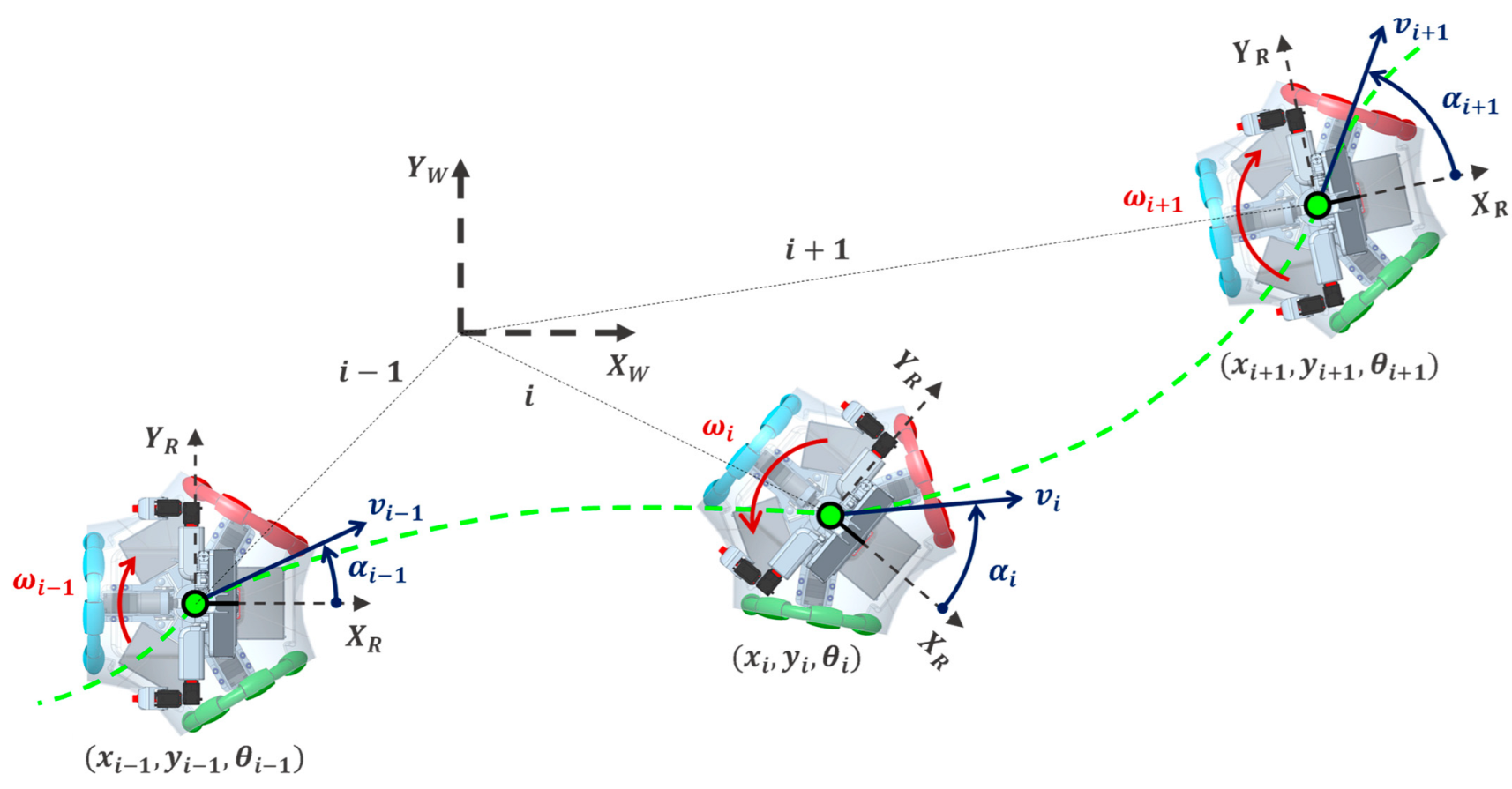
2.1. Model of the Reference Mobile Robot
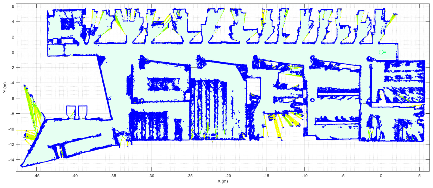
2.2. Reference Map
2.3. Navigation Tree
2.4. Dijkstra’s Algorithm
3. Implementation
3.1. Predefined Navigation Tree
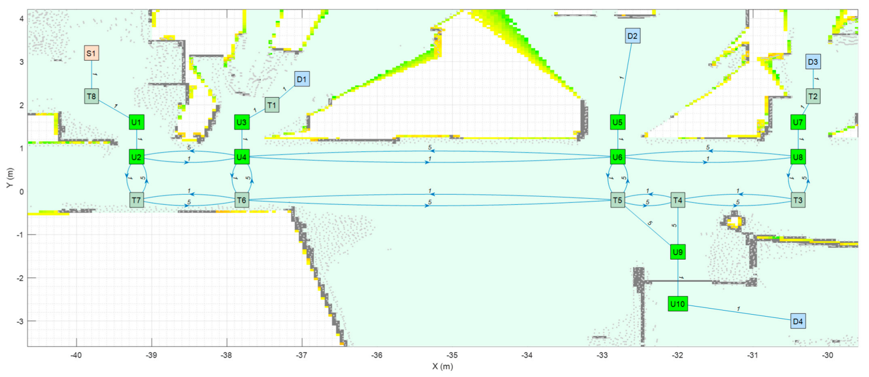
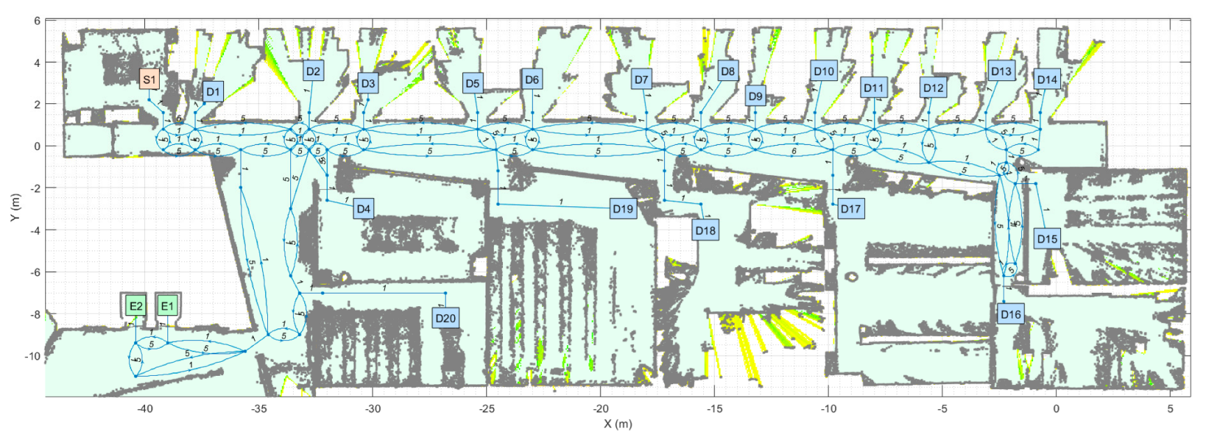
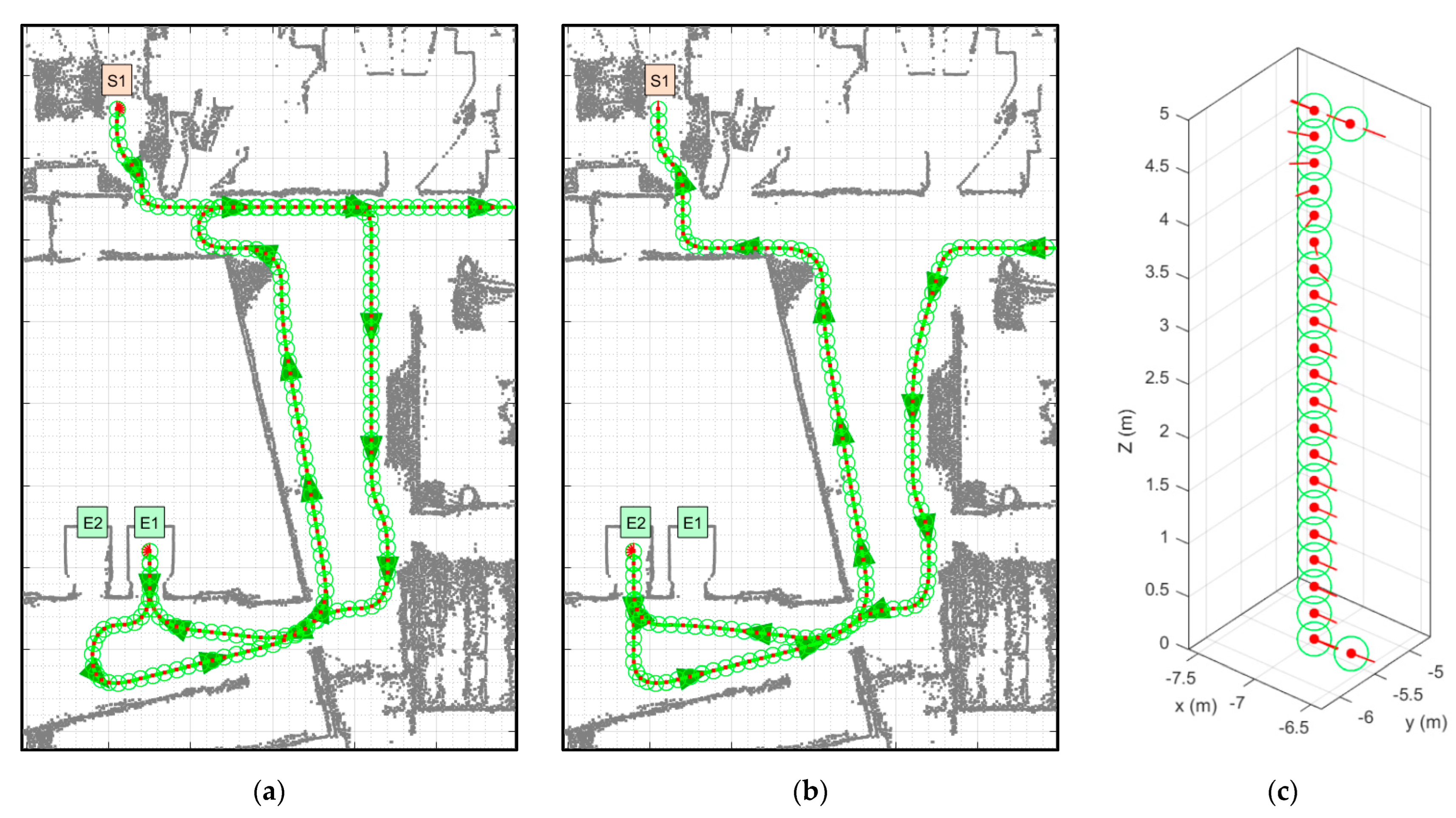
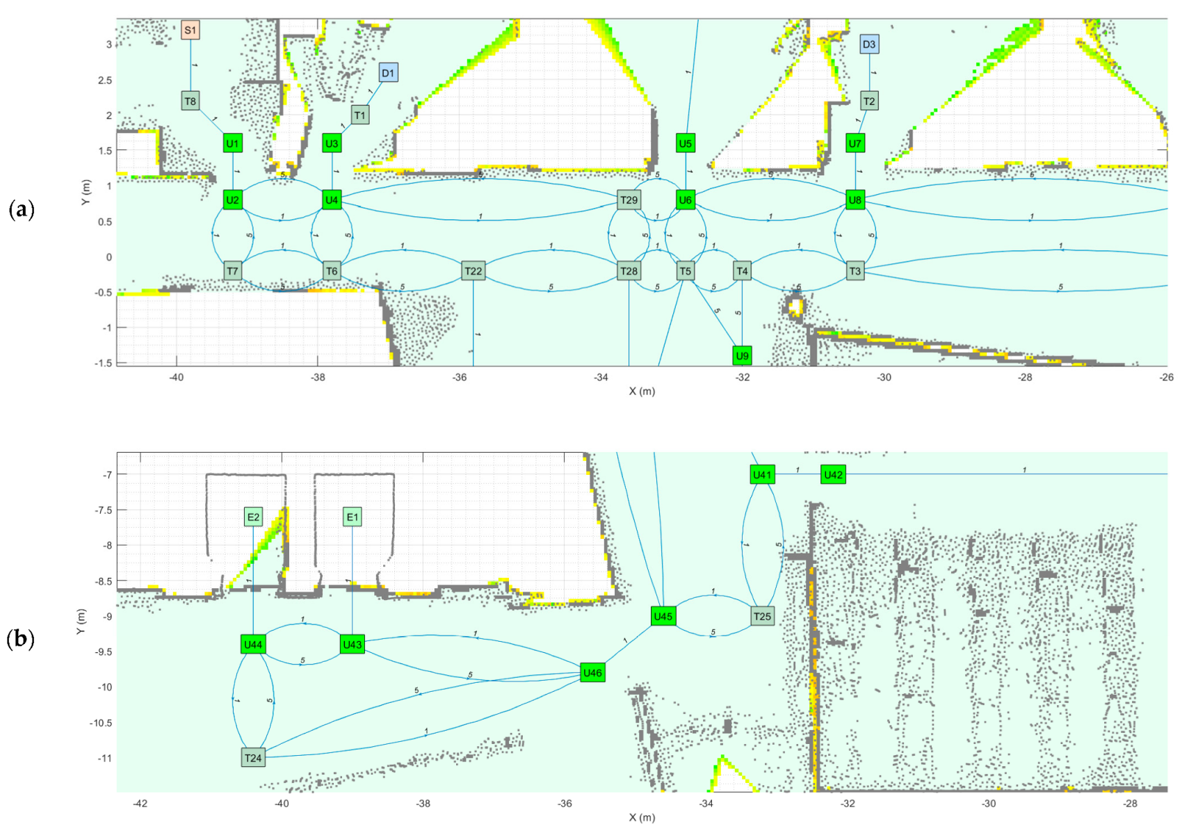
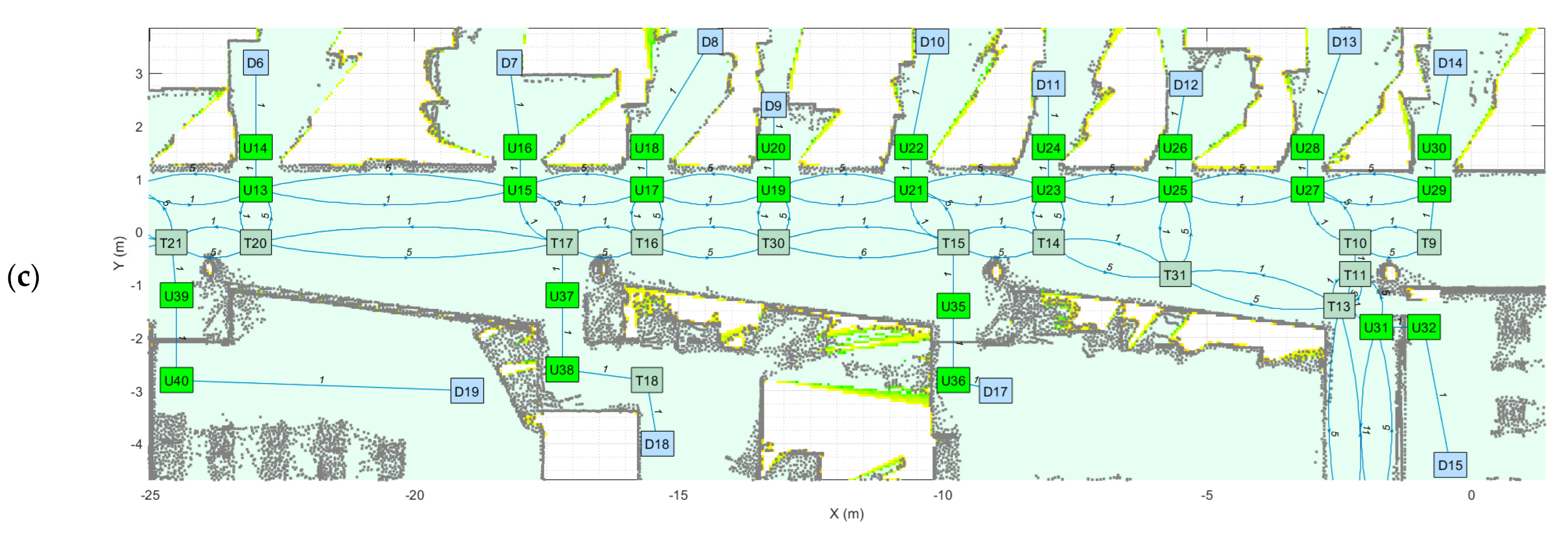
- The nodes of the navigation tree depict the position of the main pick-up points, destination points, doors and elevators. The nodes are precisely referenced in the point cloud map of the floor of the building (Figure 2).
- The segments of the navigation tree depict straight trajectories between the linked nodes. During the creation of the navigation tree, trajectory nodes can be added to define a sequence of straight segments and avoid fixed furniture obstacles.
3.2. Path Planning in a Multi-Story Building
3.3. Motion Planning in a Multi-Story Building
4. Results
5. Discussion and Conclusions
Supplementary Materials
Author Contributions
Funding
Data Availability Statement
Conflicts of Interest
References
- Statista. Retail E-Commerce Sales Growth Worldwide 2017–2027. Available online: https://www.statista.com/statistics/288487/forecast-of-global-b2c-e-commerce-growth/ (accessed on 19 September 2023).
- Leyerer, M.; Sonneberg, M.; Heumann, M.; Breitner, M. Decision support for sustainable and resilience-oriented urban parcel delivery. EURO J. Decis. Process. 2019, 7, 267–300. [Google Scholar] [CrossRef]
- Chen, M.; Wu, P.; Hsu, Y. An effective pricing model for the congestion alleviation of e-commerce logistics. Comput. Ind. Eng. 2019, 129, 368–376. [Google Scholar] [CrossRef]
- Cardenas, I.; Beckers, J.; Vandelslander, T.; Verhetsel, A.; Dewulf, W. Spatial characteristics of failed and successful Ecommerce deliveries in Belgian cities. In Proceedings of the ILS 2016—6th International Conference on Information Systems, Logistics and Supply Chain, Bordeaux, France, 1–4 June 2016. [Google Scholar]
- Langevin, A.; Mbaraga, P.; Campbell, J. Continuous approximation models in freight distribution: An overview. Transp. Res. Part B Methodol. 1996, 30, 163–188. [Google Scholar] [CrossRef]
- Boysen, N.; Fedtke, S.; Schwerdfeger, S. Last-mile delivery concepts: A survey from an operational research perspective. OR Spectr. 2021, 43, 1–58. [Google Scholar] [CrossRef]
- Jiang, L.; Mahmassani, H. City logistics. Transp. Res. Rec. J. Transp. Res. Board 2014, 2410, 85–95. [Google Scholar] [CrossRef]
- Dablanc, L.; Diziain, D.; Levifve, H. Urban freight consultations in the Paris region. Eur. Transp. Res. Rev. 2011, 3, 47–57. [Google Scholar] [CrossRef]
- Anderluh, A.; Hemmelmayr, V.C.; Rüdiger, D. Analytic hierarchy process for city hub location selection—The Viennese case. Transp. Res. Procedia 2020, 46, 77–84. [Google Scholar] [CrossRef]
- Li, L.; He, X.; Keoleian, G.A.; Kim, H.C.; De Kleine, R.; Wallington, T.J.; Kemp, N.J. Life cycle greenhouse gas emissions for last-mile parcel delivery by automated vehicles and robots. Environ. Sci. Technol. 2021, 55, 11360–11367. [Google Scholar] [CrossRef]
- Himstedt, B.; Meisel, F. Parcel delivery systems for city logistics: A cost-based comparison between different transportation technologies. Logist. Res. 2023, 16. [Google Scholar] [CrossRef]
- Mohammad, W.A.M.; Diab, Y.N.; Elomri, A.; Triki, C. Innovative solutions in last mile delivery: Concepts, practices, challenges, and future directions. Supply Chain. Forum Int. J. 2023, 24, 151–169. [Google Scholar] [CrossRef]
- Kim, J.; Moon, H.; Jung, H. Drone-Based Parcel Delivery Using the Rooftops of City Buildings: Model and Solution. Appl. Sci. 2020, 10, 4362. [Google Scholar] [CrossRef]
- Fragapane, G.; de Koster, R.; Sgarbossa, F.; Strandhagen, J.-O. Planning and control of autonomous mobile robots for intralogistics: Literature review and research agenda. Eur. J. Oper. Res. 2021, 294, 405–426. [Google Scholar] [CrossRef]
- Poeting, M.; Schaudt, S.; Clausen, U.A. Comprehensive Case Study in Last-Mile Delivery Concepts for Parcel Robots. In Proceedings of the Winter Simulation Conference (WSC), National Harbor, MD, USA, 8–11 December 2019. [Google Scholar] [CrossRef]
- Abrar, M.M.; Islam, R.; Shanto, M.A.H. An Autonomous Delivery Robot to Prevent the Spread of Coronavirus in Product Delivery System. In Proceedings of the IEEE Annual Ubiquitous Computing, Electronics & Mobile Communication Conference (UEMCON), New York, NY, USA, 28–31 October 2020. [Google Scholar] [CrossRef]
- Samouh, F.; Gluza, V.; Djavadian, S.; Meshkani, S.; Farooq, B. Multimodal Autonomous Last-Mile Delivery System Design and Application. In Proceedings of the IEEE International Smart Cities Conference (ISC2), Piscataway, NJ, USA, 28 September–1 October 2020. [Google Scholar] [CrossRef]
- Gao, F.; Cheng, Y.; Gao, M.; Ma, C.; Liu, H.; Ren, Q.; Zhao, Z. Design and Implementation of an Autonomous Driving Delivery Robot. In Proceedings of the Chinese Control Conference (CCC), Hefei, China, 25–27 July 2022. [Google Scholar] [CrossRef]
- Hutter, M.; Gehring, C.; Lauber, A.; Gunther, F.; Bellicoso, C.D.; Tsounis, V.; Meyer, K. Anymal-toward legged robots for harsh environments. Adv. Rob. 2017, 31, 918–931. [Google Scholar] [CrossRef]
- Castillo, G.A.; Weng, B.; Zhang, W.; Hereid, A. Robust Feedback Motion Policy Design Using Reinforcement Learning on a 3D Digit Bipedal Robot. In Proceedings of the IEEE/RSJ International Conference on Intelligent Robots and Systems (IROS), Prague, Czech Republic, 27 September–1 October 2021. [Google Scholar] [CrossRef]
- Galindo, C.; Fernández-Madrigal, J.-A.; González, J.; Saffiotti, A. Robot task planning using semantic maps. Robot. Auton. Syst. 2008, 56, 955–966. [Google Scholar] [CrossRef]
- Abed, M.; Farouq, O.; Doori, Q.A. A Review on Path Planning Algorithms for Mobile Robots. Eng. Technol. J. 2021, 39, 804–820. [Google Scholar] [CrossRef]
- Rafai, A.N.A.; Adzhar, N.; Jaini, N.I.; Ding, B. A Review on Path Planning and Obstacle Avoidance Algorithms for Autonomous Mobile Robots. J. Robot. 2022, 2022, 2538220. [Google Scholar] [CrossRef]
- Fouque, C.; Bonnifait, P. On the use of 2D navigable maps for enhancing ground vehicle localization. In Proceedings of the 2009 IEEE/RSJ International Conference on Intelligent Robots and Systems, St. Louis, MO, USA, 10–15 October 2009. [Google Scholar] [CrossRef]
- Liu, L.; Wang, X.; Yang, X.; Liu, H.; Li, J.; Wang, P. Path planning techniques for mobile robots: Review and prospect. Expert Syst. Appl. 2023, 227, 120254. [Google Scholar] [CrossRef]
- De Ryck, M.; Versteyhe, M.; Debrouwere, F. Automated guided vehicle systems, state-of-the-art control algorithms and techniques. J. Manuf. Syst. 2020, 54, 152–173. [Google Scholar] [CrossRef]
- Kim, J.-T.; Choi, Y.-H.; Lee, J.; Hong, S.-H. Floor-to-floor navigation for a mobile robot. In Proceedings of the 2013 10th International Conference on Ubiquitous Robots and Ambient Intelligence (URAI), Jeju, Republic of Korea, 30 October–2 November 2013. [Google Scholar] [CrossRef]
- Zhang, H.; Tao, W.; Huang, J.; Zheng, R. Development of An In-building Transport Robot for Autonomous Usage of Elevators. In Proceedings of the 2018 IEEE International Conference on Intelligence and Safety for Robotics (ISR), Shenyang, China, 24–27 August 2018. [Google Scholar] [CrossRef]
- Law, W.-t.; Li, K.-s.; Fan, K.-w.; Mo, T.; Poon, C.-k. Friendly Elevator Co-rider: An HRI Approach for Robot-Elevator Interaction. In Proceedings of the 17th ACM/IEEE International Conference on Human-Robot Interaction (HRI), Sapporo, Japan, 7–10 March 2022. [Google Scholar] [CrossRef]
- Rubies, E.; Bitriá, R.; Clotet, E.; Palacín, J. Non-Contact and Non-Intrusive Add-on IoT Device for Wireless Remote Elevator Control. Appl. Sci. 2023, 13, 3971. [Google Scholar] [CrossRef]
- Palacín, J.; Bitriá, R.; Rubies, E.; Clotet, E. A Procedure for Taking a Remotely Controlled Elevator with an Autonomous Mobile Robot Based on 2D LIDAR. Sensors 2023, 23, 6089. [Google Scholar] [CrossRef]
- Arisumi, H.; Chardonnet, J.-R.; Yokoi, K. Whole-body motion of a humanoid robot for passing through a door—Opening a door by impulsive force. In Proceedings of the 2009 IEEE/RSJ International Conference on Intelligent Robots and Systems, St. Louis, MO, USA, 10–15 October 2009. [Google Scholar] [CrossRef]
- Digioia, G.; Arisumi, H.; Yokoi, K. Trajectory planner for a humanoid robot passing through a door. In Proceedings of the 9th IEEE-RAS International Conference on Humanoid Robots, Paris, France, 7–10 December 2009. [Google Scholar] [CrossRef]
- Kwak, N.; Arisumi, H.; Yokoi, K. Visual recognition of a door and its knob for a humanoid robot. In Proceedings of the IEEE International Conference on Robotics and Automation, Shanghai, China, 9–13 May 2011. [Google Scholar] [CrossRef]
- Arisumi, H.; Kwak, N.; Yokoi, K. Systematic touch scheme for a humanoid robot to grasp a door knob. In Proceedings of the IEEE International Conference on Robotics and Automation, Shanghai, China, 9–13 May 2011. [Google Scholar] [CrossRef]
- Banerjee, N.; Long, X.; Du, R.; Polido, F.; Feng, S.; Atkeson, C.G.; Gennert, M.; Padir, T. Human-supervised control of the ATLAS humanoid robot for traversing doors. In Proceedings of the IEEE-RAS 15th International Conference on Humanoid Robots (Humanoids), Seoul, Republic of Korea, 3–5 November 2015. [Google Scholar] [CrossRef]
- Thrun, S. Robotic mapping: A survey. In Exploring Artificial Intelligence in the New Millenium; Lakemeyer, G., Nebel, B., Eds.; Kaufmann Publishers: San Francisco, CA, USA, 2003. [Google Scholar]
- Chen, C.; Cheng, Y. Research on Map Building by Mobile Robots. In Proceedings of the 2008 International Symposium on Intelligent Information Technology Application, Shanghai, China, 20–22 December 2008. [Google Scholar] [CrossRef]
- Asada, M. Map building for a mobile robot from sensory data. IEEE Trans. Syst. Man Cybern. 1990, 37, 1326–1336. [Google Scholar] [CrossRef]
- Kuipers, B.; Byun, Y.-T. A robot exploration and mapping strategy based on a semantic hierarchy of spatial representations. Robot. Auton. Syst. 1991, 8, 47–63. [Google Scholar] [CrossRef]
- Kröse, B.J.A.; Vlassis, N.; Bunschoten, R.; Motomura, Y. A probabilistic model for appearance-based robot localization. Image Vis. Comput. 2001, 19, 381–391. [Google Scholar] [CrossRef]
- Jacky, C.H.; George, L.C.S.; Charlie, H.Y.; Lu, Y.-H. Multi-robot SLAM with topological/metric maps. In Proceedings of the IEEE/RSJ International Conference on Intelligent Robots and Systems, San Diego, CA, USA, 29 October–2 November 2007. [Google Scholar] [CrossRef]
- Choset, H.; Nagatani, K. Topological simultaneous localization and mapping (SLAM): Toward exact localization without explicit localization. IEEE Trans. Robot. Autom. 2001, 17, 125–137. [Google Scholar] [CrossRef]
- Lee, D.; Chung, W.; Kim, M. A reliable position estimation method of the service robot by map matching. In Proceedings of the IEEE International Conference on Robotics and Automation, Taipei, Taiwan, 14–19 September 2003. [Google Scholar] [CrossRef]
- Zhou, J.-H.; Lin, H.-Y. A self-localization and path planning technique for mobile robot navigation. In Proceedings of the 9th World Congress on Intelligent Control and Automation, Taipei, Taiwan, 21–25 June 2011. [Google Scholar] [CrossRef]
- Kubota, N. Topological approaches for simultaneous localization and mapping. In Proceedings of the 6th International Conference on Informatics, Electronics and Vision & 2017 International Symposium in Computational Medical and Health Technology, Himeji, Japan, 1–3 September 2017. [Google Scholar] [CrossRef]
- Warrier, A.R.; Nedunghat, P.; Bera, M.K.; Nath, K. Implementation of Classical Path Planning Algorithms for Mobile Robot Navigation: A Comprehensive Comparison. In Proceedings of the International Conference on Electrical, Computer, Communications and Mechatronics Engineering, Maldives, 16–18 November 2022. [Google Scholar] [CrossRef]
- Sundar, K.; Misra, S.; Rathinam, S.; Sharma, R. Routing unmanned vehicles in GPS-denied environments. In Proceedings of the International Conference on Unmanned Aircraft Systems (ICUAS), Miami, FL, USA, 13–16 June 2017. [Google Scholar] [CrossRef]
- Žunić, E.; Hindija, H.; Beširević, A.; Hodžić, K.; Delalić, S. Improving Performance of Vehicle Routing Algorithms using GPS Data. In Proceedings of the 14th Symposium on Neural Networks and Applications (NEUREL), Belgrade, Serbia, 20–21 November 2018. [Google Scholar] [CrossRef]
- Aqel, M.O.A.; Marhaban, M.H.; Saripan, M.I.; Ismail, N.B. Review of visual odometry: Types, approaches, challenges, and applications. SpringerPlus 2016, 5, 1897. [Google Scholar] [CrossRef] [PubMed]
- Bârsan, I.A.; Liu, P.; Pollefeys, M.; Geiger, A. Robust dense mapping for large-scale dynamic environments. In Proceedings of the IEEE International Conference on Robotics and Automation, Brisbane, QLD, Australia, 21–25 May 2018. [Google Scholar] [CrossRef]
- Ji, K.; Chen, H.; Di, H.; Gong, J.; Xiong, G.; Qi, J.; Yi, T. CPFG-SLAM: A robust simultaneous localization and mapping based on LIDAR in off-road environment. In Proceedings of the IEEE Intelligent Vehicles Symposium (IV), Changshu, China, 26–30 June 2018. [Google Scholar] [CrossRef]
- Du, S.; Li, Y.; Li, X.; Wu, M. LiDAR Odometry and Mapping Based on Semantic Information for Outdoor Environment. Remote Sens. 2021, 13, 2864. [Google Scholar] [CrossRef]
- Chen, Y.; Medioni, G. Object modeling by registration of multiple range images. In Proceedings of the IEEE International Conference on Robotics and Automation, Sacramento, CA, USA, 9–11 April 1991. [Google Scholar] [CrossRef]
- Besl, P.J.; McKay, N.D. A Method for Registration of 3-D Shapes. IEEE Trans. Pattern Anal. Mach. Intell. 1992, 14, 239–256. [Google Scholar] [CrossRef]
- Yokozuka, M.; Koide, K.; Oishi, S.; Banno, A. LiTAMIN: LiDAR-Based Tracking and Mapping by Stabilized ICP for Geometry Approximation with Normal Distributions. In Proceedings of the IEEE/RSJ International Conference on Intelligent Robots and Systems (IROS), Las Vegas, NV, USA, 24 October 2020–24 January 2021. [Google Scholar] [CrossRef]
- Koide, K.; Miura, J.; Menegatti, E. A portable three-dimensional LIDAR-based system for long-term and wide-area people behavior measurement. Int. J. Adv. Robot. Syst. 2019, 16. [Google Scholar] [CrossRef]
- Behley, J.; Stachniss, C. Efficient Surfel-Based SLAM using 3D Laser Range Data in Urban Environments. In Proceedings of the International Conference on Robotics: Science and Systems (RSS), Pittsburgh, PA, USA, 26–30 June 2018. [Google Scholar] [CrossRef]
- Park, C.; Moghadam, P.; Kim, S.; Elfes, A.; Fookes, C.; Sridharan, S. Elastic LiDAR Fusion: Dense Map-Centric Continuous-Time SLAM. In Proceedings of the International Conference on Robotics and Automation (ICRA), Brisbane, Australia, 21–25 May 2017. [Google Scholar] [CrossRef]
- Whelan, T.; Leutenegger, S.; Moreno, R.F.S.; Glocker, B.; Davison, A.J. ElasticFusion: Dense SLAM without a Pose Graph. In Proceedings of the International Conference of Robotics: Science and Systems (RSS), Rome, Italy, 13–15 July 2015. [Google Scholar] [CrossRef]
- Moosmann, F.; Stiller, C. Velodyne SLAM. In Proceedings of the 2011 IEEE Intelligent Vehicles Symposium (IV), Baden-Baden, Germany, 5–9 June 2011. [Google Scholar] [CrossRef]
- Droeschel, D.; Behnke, S. Efficient Continuous-time SLAM for 3D Lidar-based Online Mapping. In Proceedings of the International Conference on Robotics and Automation (ICRA), Brisbane, Australia, 21–25 May 2018. [Google Scholar] [CrossRef]
- Palacín, J.; Martínez, D.; Rubies, E.; Clotet, E. Mobile Robot Self-Localization with 2D Push-Broom LIDAR in a 2D Map. Sensors 2020, 20, 2500. [Google Scholar] [CrossRef]
- Zhang, J.; Singh, S. LOAM: Lidar Odometry and Mapping in Real-time. In Proceedings of the International Conference of Robotics: Science and Systems (RSS), Berkeley, CA, USA, 12–16 July 2014. [Google Scholar] [CrossRef]
- Zhang, J.; Singh, S. Low-drift and Real-time Lidar Odometry and Mapping. Auton. Robot. 2017, 41, 401–416. [Google Scholar] [CrossRef]
- Shan, T.; Englot, B. LeGO-LOAM: Lightweight and Ground- Optimized Lidar Odometry and Mapping on Variable Terrain. In Proceedings of the IEEE/RSJ International Conference on Intelligent Robots and Systems (IROS), Madrid, Spain, 1–5 October 2018. [Google Scholar] [CrossRef]
- Ye, H.; Chen, Y.; Liu, M. Tightly Coupled 3D Lidar Inertial Odometry and Mapping. In Proceedings of the International Conference on Robotics and Automation, Montreal, QC, Canada, 20–24 May 2019. [Google Scholar] [CrossRef]
- Shan, T.; Englot, B.; Meyers, D.; Wang, W.; Ratti, C.; Rus, D. LIO-SAM: Tightly-coupled Lidar Inertial Odometry via Smoothing and Mapping. In Proceedings of the IEEE/RSJ International Conference on Intelligent Robots and Systems (IROS), Las Vegas, NV, USA, 24 October 2020–24 January 2021. [Google Scholar] [CrossRef]
- Qin, C.; Ye, H.; Pranata, C.E.; Han, J.; Zhang, S.; Liu, M. LINS: A Lidar-Inertial State Estimator for Robust and Efficient Navigation. In Proceedings of the IEEE International Conference on Robotics and Automation (ICRA), Virtual (Online), 31 May–31 August 2020. [Google Scholar] [CrossRef]
- LeCun, Y.; Bengio, Y.; Hinton, G. Deep Learning. Nature 2015, 521, 436–444. [Google Scholar] [CrossRef] [PubMed]
- Zheng, C.; Lyu, Y.; Li, M.; Zhang, Z. Lodonet: A deep neural network with 2D keypoint matching for 3d lidar odometry estimation. In Proceedings of the ACM International Conference on Multimedia, Virtual (Online), 12–16 October 2020. [Google Scholar] [CrossRef]
- Li, Z.; Wang, N. Dmlo: Deep matching lidar odometry. In Proceedings of the IEEE/RSJ International Conference on Intelligent Robots and Systems (IROS), Virtual (Online), 24 October 2020–24 January 2021. [Google Scholar] [CrossRef]
- Li, Q.; Chen, S.; Wang, C.; Li, X.; Wen, C.; Cheng, M.; Li, J. LO-net: Deep real-time lidar odometry. In Proceedings of the IEEE/CVF Conference on Computer Vision and Pattern Recognition, Long Beach, CA, USA, 15–20 June 2019. [Google Scholar] [CrossRef]
- Nubert, J.; Khattak, S.; Hutter, M. Self-supervised learning of lidar odometry for robotic applications. In Proceedings of the IEEE International Conference on Robotics and Automation (ICRA), Xi’an, China, 30 May–5 June 2021. [Google Scholar] [CrossRef]
- Wang, M.; Saputra, M.R.U.; Zhao, P.; Gusmao, P.; Yang, B.; Chen, C.; Markham, A.; Trigoni, N. Deeppco: End-to-end point cloud odometry through deep parallel neural network. In Proceedings of the EEE/RSJ International Conference on Intelligent Robots and Systems (IROS), Macau, China, 3–8 November 2019. [Google Scholar] [CrossRef]
- Cho, Y.; Kim, G.; Kim, A. Unsupervised geometry-aware deep lidar odometry. In Proceedings of the IEEE International Conference on Robotics and Automation (ICRA), Paris, France, 31 May–31 August 2020. [Google Scholar] [CrossRef]
- Wang, G.; Wu, X.; Liu, Z.; Wang, H. Pwclo-net: Deep lidar odometry in 3d point clouds using hierarchical embedding mask optimization. In Proceedings of the IEEE/CVF Conference on Computer Vision and Pattern Recognition (CVPR), Nashville, TN, USA, 20–25 June 2021. [Google Scholar] [CrossRef]
- Wang, C.; Liu, X.; Yang, X.; Hu, F.; Jiang, A.; Yang, C. Trajectory Tracking of an Omni-Directional Wheeled Mobile Robot Using a Model Predictive Control Strategy. Appl. Sci. 2018, 8, 231. [Google Scholar] [CrossRef]
- Palacín, J.; Rubies, E.; Clotet, E.; Martínez, D. Evaluation of the Path-Tracking Accuracy of a Three-Wheeled Omnidirectional Mobile Robot Designed as a Personal Assistant. Sensors 2021, 21, 7216. [Google Scholar] [CrossRef] [PubMed]
- Kang, J.G.; An, S.Y.; Oh, S.Y. Navigation strategy for the service robot in the elevator environment. In Proceedings of the International Conference on Control, Automation and Systems, Seoul, Republic of Korea, 17–20 October 2007; pp. 1092–1097. [Google Scholar] [CrossRef]
- van Toll, W.; Cook, A.F.; Geraerts, R. Navigation meshes for realistic multi-layered environments. In Proceedings of the IEEE/RSJ International Conference on Intelligent Robots and Systems, San Francisco, CA, USA, 25–30 September 2011; pp. 3526–3532. [Google Scholar] [CrossRef]
- Zhang, Q.; Wu, X.; Liu, B.; Adiwahono, A.H.; Dung, T.A.; Chang, T.W. A hierarchical topological planner for multi-storey building navigation. In Proceedings of the IEEE International Conference on Advanced Intelligent Mechatronics (AIM), Busan, Republic of Korea, 7–11 July 2015; pp. 731–736. [Google Scholar] [CrossRef]
- Liu, K.; Motta, G.; Ma, T.; Guo, T. Multi-floor Indoor Navigation with Geomagnetic Field Positioning and Ant Colony Optimization Algorithm. In Proceedings of the IEEE Symposium on Service-Oriented System Engineering (SOSE), Oxford, UK, 29 March–2 April 2016; pp. 314–323. [Google Scholar] [CrossRef]
- Joo, S.H.; Manzoor, S.; Kuc, T.Y. A Semantic Navigation Framework for Multi-Floor Building Environment. In Proceedings of the International Conference on Control, Automation and Systems (ICCAS), Jeju, Republic of Korea, 12–15 October 2021; pp. 1543–1545. [Google Scholar] [CrossRef]
- Li, Z. Using MDP to Find the Best Path in Multi-floor World. In Proceedings of the IEEE International Conference on Frontiers Technology of Information and Computer (ICFTIC), Greenville, SC, USA, 12–14 November 2021; pp. 447–452. [Google Scholar] [CrossRef]
- Yuan, J.; Jiao, B.; Wang, L. Indoor and outdoor integrated path planning algorithm for multi-storey buildings. In Proceedings of the 2022 World Automation Congress (WAC), San Antonio, TX, USA, 11–15 October 2022; pp. 336–340. [Google Scholar] [CrossRef]
- Fransen, K.; van Eekelen, J. Efficient path planning for automated guided vehicles using A* (Astar) algorithm incorporating turning costs in search heuristic. Int. J. Prod. Res. 2023, 61, 707–725. [Google Scholar] [CrossRef]
- Dijkstra, E.W. A note on two problems in connexion with graphs. Numer. Math. 1959, 1, 269–271. [Google Scholar] [CrossRef]
- Floyd, R.W. Algorithm 97: Shortest Path. Commun. ACM 1962, 5, 345. [Google Scholar] [CrossRef]
- Hart, P.E.; Nilsson, N.J.; Raphael, B. A Formal Basis for the Heuristic Determination of Minimum Cost Paths. IEEE Trans. Syst. Sci. Cybern. 1968, 4, 100–107. [Google Scholar] [CrossRef]
- Holland, J.H. Genetic Algorithms and Adaptation. In Adaptive Control of Ill-Defined Systems; Selfridge, O.G., Rissland, E.L., Arbib, M.A., Eds.; NATO Conference Series; Springer: Boston, MA, USA, 1984; Volume 16. [Google Scholar] [CrossRef]
- Kirkpatrick, S.; Gelatt, C.D.; Vecchi, M.P. Optimization by Simulated Annealing. Science 1983, 220, 671–680. [Google Scholar] [CrossRef]
- Lawler, E.L.; Wood, D.E. Branch-And-Bound Methods: A Survey. Oper. Res. 1966, 14, 699–719. Available online: http://www.jstor.org/stable/168733 (accessed on 12 September 2023). [CrossRef]
- Griffiths, I.J.; Mehdi, Q.H.; Wang, T.; Gough, N.E. A Genetic Algorithm for Path Planning. IFAC Proc. Vol. 1997, 30, 485–490. [Google Scholar] [CrossRef]
- Lamini, C.; Benhlima, S.; Elbekri, A. Genetic Algorithm Based Approach for Autonomous Mobile Robot Path Planning. Procedia Comput. Sci. 2018, 127, 180–189. [Google Scholar] [CrossRef]
- Kusuma, M.; Riyanto; Machbub, C. Humanoid Robot Path Planning and Rerouting Using A-Star Search Algorithm. In Proceedings of the IEEE International Conference on Signals and Systems, Bandung, Indonesia, 16–18 July 2019. [Google Scholar] [CrossRef]
- Ganeshmurthy, M.S.; Suresh, G.R. Path planning algorithm for autonomous mobile robot in dynamic environment. In Proceedings of the 3rd International Conference on Signal Processing, Communication and Networking, Chennai, India, 26–28 March 2015. [Google Scholar] [CrossRef]
- Tsuzuki, M.S.G.; Martins, T.C.; Takase, F.K. Robot path planning using simulated annealing. IFAC Proc. Vol. 2006, 39, 175–180. [Google Scholar] [CrossRef]
- Miao, H.; Tian, Y.-C. Robot path planning in dynamic environments using a simulated annealing based approach. In Proceedings of the 10th International Conference on Control, Automation, Robotics and Vision, Hanoi, Vietnam, 17–20 December 2008. [Google Scholar] [CrossRef]
- Kim, J.; Jung, H. Robot Routing Problem of Last-Mile Delivery in Indoor Environments. Appl. Sci. 2022, 12, 9111. [Google Scholar] [CrossRef]
- Palacín, J.; Rubies, E.; Clotet, E. The Assistant Personal Robot Project: From the APR-01 to the APR-02 Mobile Robot Prototypes. Designs 2022, 6, 66. [Google Scholar] [CrossRef]
- Palacín, J.; Martínez, D.; Rubies, E.; Clotet, E. Suboptimal Omnidirectional Wheel Design and Implementation. Sensors 2021, 21, 865. [Google Scholar] [CrossRef] [PubMed]
- Palacín, J.; Clotet, E.; Martínez, D.; Martínez, D.; Moreno, J. Extending the Application of an Assistant Personal Robot as a Walk-Helper Tool. Robotics 2019, 8, 27. [Google Scholar] [CrossRef]
- Mori, Y.; Yokoyama, S.; Yamashita, T.; Kawamura, H.; Mori, M. Obstacle Avoidance Using Depth Imaging for Forearm-Supported Four-Wheeled Walker with Walking Assist. In Proceedings of the International Conference on Ubiquitous Robots (UR), Honolulu, HI, USA, 25–28 June 2023; pp. 544–551. [Google Scholar] [CrossRef]
- Tian, P.; Zhang, Y.N.; Zhang, J.; Yan, N.M.; Zeng, W. Research on Simulation of Motion Compensation for 8×8 Omnidirectional Platform Based on Back Propagation Network. Appl. Mech. Mater. 2013, 299, 44–47. [Google Scholar] [CrossRef]
- Peng, T.; Qian, J.; Zi, B.; Liu, J.; Wang, X. Mechanical Design and Control System of an Omni-directional Mobile Robot for Material Conveying. Procedia CIRP 2016, 56, 412–415. [Google Scholar] [CrossRef]
- Wang, Z.; Yang, G.; Su, X.; Schwager, M. OuijaBots: Omnidirectional Robots for Cooperative Object Transport with Rotation Control Using No Communication. In Distributed Autonomous Robotic Systems; Groß, R., Kolling, A., Berman, S., Frazzoli, E., Martinoli, A., Matsuno, F., Gauci, M., Eds.; Springer: Cham, Switzerland, 2018; Volume 6. [Google Scholar] [CrossRef]
- Li, Y.; Ge, S.; Dai, S.; Zhao, L.; Yan, X.; Zheng, Y.; Shi, Y. Kinematic Modeling of a Combined System of Multiple Mecanum-Wheeled Robots with Velocity Compensation. Sensors 2020, 20, 75. [Google Scholar] [CrossRef]
- Purwin, O.; D’Andrea, R. Trajectory generation and control for four wheeled omnidirectional vehicles. Robot. Auton. Syst. 2006, 54, 13–22. [Google Scholar] [CrossRef]
- Kim, K.B.; Kim, B.K. Minimum-Time Trajectory for Three-Wheeled Omnidirectional Mobile Robots Following a Bounded-Curvature Path with a Referenced Heading Profile. IEEE Trans. Robot. 2011, 27, 800–808. [Google Scholar] [CrossRef]
- Jia, W.; Zhao, W.; Song, Z.; Li, Z. Object Servoing of Differential-Drive Robots. In Proceedings of the Chinese Control and Decision Conference (CCDC), Kunming, China, 22–24 May 2021. [Google Scholar] [CrossRef]
- Bitriá, R.; Palacín, J. Optimal PID Control of a Brushed DC Motor with an Embedded Low-Cost Magnetic Quadrature Encoder for Improved Step Overshoot and Undershoot Responses in a Mobile Robot Application. Sensors 2022, 22, 7817. [Google Scholar] [CrossRef] [PubMed]
- Palacín, J.; Rubies, E.; Clotet, E. Systematic Odometry Error Evaluation and Correction in a Human-Sized Three-Wheeled Omnidirectional Mobile Robot Using Flower-Shaped Calibration Trajectories. Appl. Sci. 2022, 12, 2606. [Google Scholar] [CrossRef]
- Clotet, E.; Palacín, J. SLAMICP Library: Accelerating Obstacle Detection in Mobile Robot Navigation via Outlier Monitoring following ICP Localization. Sensors 2023, 23, 6841. [Google Scholar] [CrossRef] [PubMed]
- Styan, G.P.H. Hadamard products and multivariate statistical analysis. Linear Algebra Its Appl. 1973, 6, 217–240. [Google Scholar] [CrossRef]
- Makariye, N. Towards shortest path computation using Dijkstra algorithm. In Proceedings of the 2017 International Conference on IoT and Application (ICIOT), Nagapattinam, India, 19–20 May 2017. [Google Scholar] [CrossRef]
- Asadi, S.; Azimirad, V.; Eslami, A.; Ghanbari, A. A novel global optimal path planning and trajectory method based on adaptive dijkstra-immune approach for mobile robot. In Proceedings of the IEEE/ASME International Conference on Advanced Intelligent Mechatronics (AIM), Budapest, Hungary, 3–7 July 2011. [Google Scholar] [CrossRef]
- Fusic, J.S.; Ramkumar, P.; Hariharan, K. Path planning of robot using modified Dijkstra Algorithm. In Proceedings of the 2018 National Power Engineering Conference (NPEC), Madurai, India, 9–10 March 2018. [Google Scholar] [CrossRef]
- Wang, H.; Yu, Y.; Yuan, Q. Application of Dijkstra algorithm in robot path-planning. In Proceedings of the International Conference on Mechanic Automation and Control Engineering, Hohhot, China, 15–17 July 2011; pp. 1067–1069. [Google Scholar] [CrossRef]
- Li, X. Path planning of intelligent mobile robot based on Dijkstra algorithm. J. Phys. Conf. Ser. 2021, 2083, 042034. [Google Scholar] [CrossRef]
- Alshammrei, S.; Boubaker, S.; Kolsi, L. Improved Dijkstra algorithm for mobile robot path planning and obstacle avoidance. Comput. Mater. Contin. 2022, 72, 5939–5954. [Google Scholar] [CrossRef]
- Dijkstra’s Shortest Path Algorithm Explained. Available online: https://youtu.be/bZkzH5x0SKU (accessed on 1 September 2023).
- Dijkstra’s Algorithm. MATLAB Central File Exchange. Available online: https://www.mathworks.com/matlabcentral/fileexchange/134851-dijkstra (accessed on 1 September 2023).
- Khatib, O. Real-time obstacle avoidance for manipulators and mobile robots. In Proceedings of the IEEE International Conference on Robotics and Automation, St. Louis, MO, USA, 25–28 March 1985; pp. 500–505. [Google Scholar] [CrossRef]
- Zhang, Y.; Liu, K.; Gao, F.; Zhao, F. Research on Path Planning and Path Tracking Control of Autonomous Vehicles Based on Improved APF and SMC. Sensors 2023, 23, 7918. [Google Scholar] [CrossRef]
- Hough, D.G. The IEEE Standard 754: One for the History Books. Computer 2019, 52, 109–112. [Google Scholar] [CrossRef]
- Kunchev, V.; Jain, L.; Ivancevic, V.; Finn, A. Path Planning and Obstacle Avoidance for Autonomous Mobile Robots: A Review. In Knowledge-Based Intelligent Information and Engineering Systems; Gabrys, B., Howlett, R.J., Jain, L.C., Eds.; Lecture Notes in Computer Science; Springer: Berlin/Heidelberg, Germany, 2006; Volume 4252, pp. 537–544. [Google Scholar] [CrossRef]
- Anavatti, S.G.; Francis, S.L.X.; Garratt, M. Path-planning modules for Autonomous Vehicles: Current status and challenges. In Proceedings of the International Conference on Advanced Mechatronics, Intelligent Manufacture, and Industrial Automation (ICAMIMIA), Surabaya, Indonesia, 15–17 October 2015; pp. 205–214. [Google Scholar] [CrossRef]


| Graphic Representation | Node Type | Description | Position Editable in the Map |
|---|---|---|---|
 | Start | Main package pick-up node and battery charging station | No |
 | Trajectory | Intermediate trajectory node | Yes |
 | Unique | Special node used to define precise trajectories, for example, to pass through open doors | No |
 | Elevator | Placement of an elevator | No |
 | Destination | Destination node | Yes |
| Segments | Weight | ||
|---|---|---|---|
| Graphic Representation | Type | From S1 to D1 | From D1 to S1 |
 | unconnected | Infinite | Infinite |
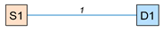 | undirected | 1.0 | 1.0 |
 | directed | 1.0 | 5.0 |
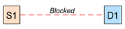 | blocked | Infinite | Infinite |
| Current Node of the Robot | Is Next Segment Blocked? | Current Delivery | Planned Path | |
|---|---|---|---|---|
| From | To | |||
| S1 | No | S1 (Package pick-up point) | D3 (Destination point) | 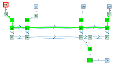 |
| U6 | Yes (Compute a new path from U6) | U6 | D3 | 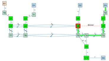 |
| D3 (Package delivery) | - | U6 | D3 | 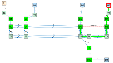 |
| D3 (Return) | No | D3 (Return to starting point) | S1 |  |
| S1 (Arrival at the departure point) | - | D3 | S1 | 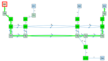 |
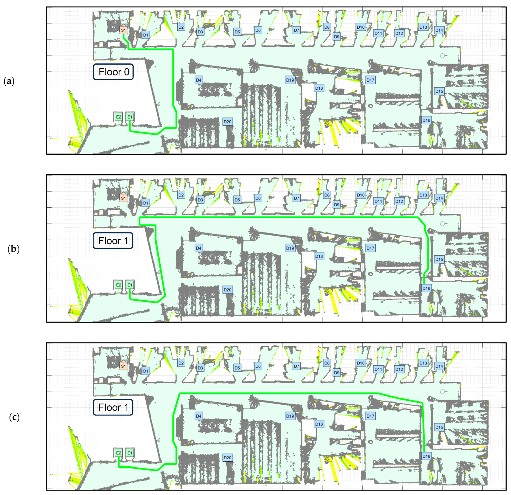
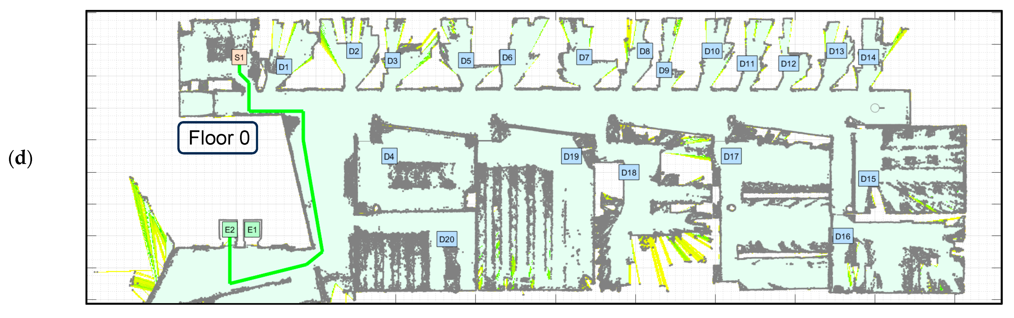
| Task | Initial Node | Destination Node | Sequence of Nodes to Visit |
|---|---|---|---|
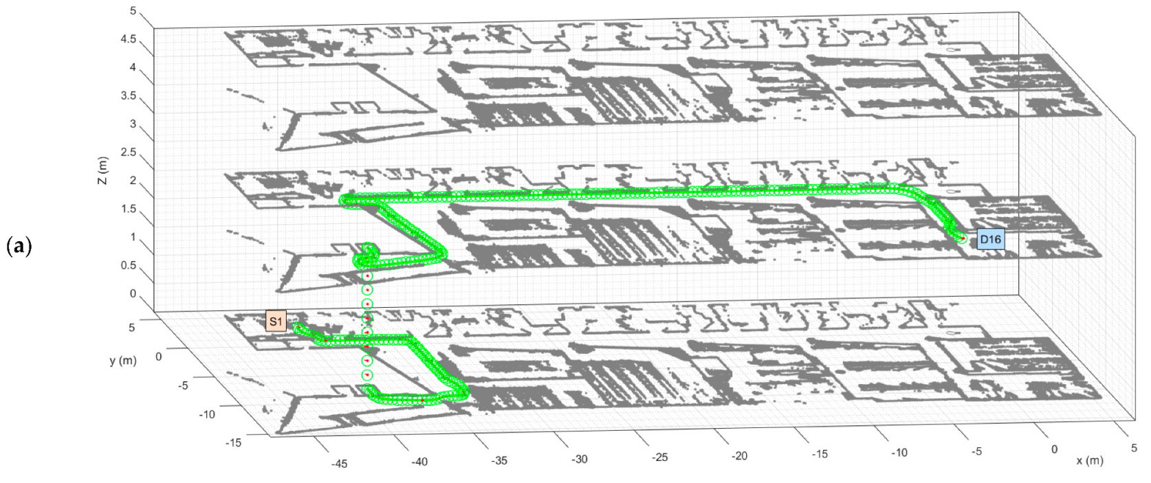
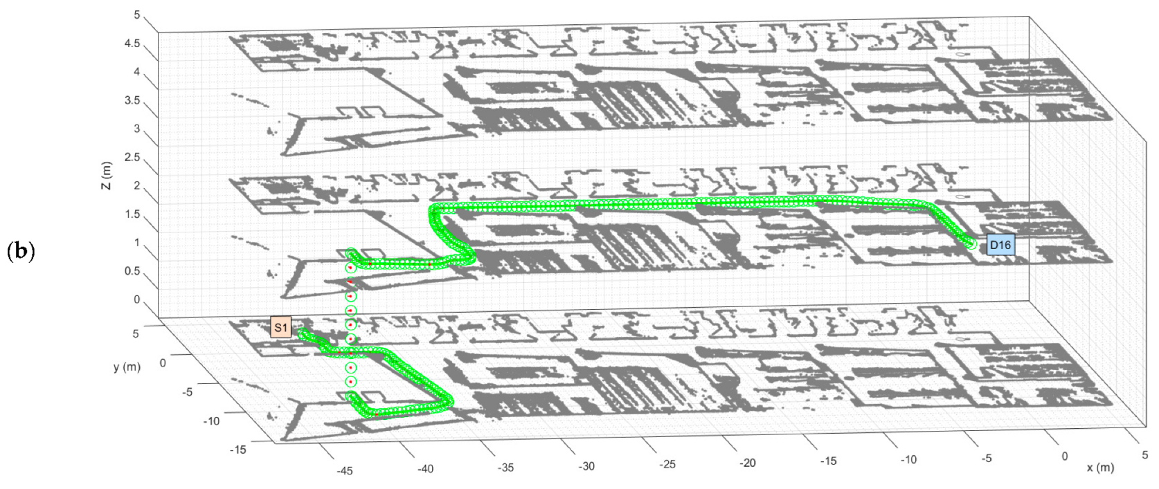
| 1 (go) | S1-F0 | D16-F1 | 1: S1-F0 2: E1-F0→F1 3: D16-F1 |
| 2 (return) | D16-F1 | S1-F0 | 1: D16-F1 2: E2-F1→F0 3: S1-F0 |
| Task | Initial Node | Destination Node | Final Node | Cumulated Path Length When Origin and Destination Are | ||
|---|---|---|---|---|---|---|
| On the Same Floor | On Different Floors | Difference | ||||
| T1 | S1 | D1 | S1 | 12.27 m | 102.13 m | 89.86 m |
| T2 | S1 | D2 | S1 | 25.72 m | 104.49 m | 78.77 m |
| T3 | S1 | D3 | S1 | 29.36 m | 108.13 m | 68.77 m |
| T4 | S1 | D4 | S1 | 29.24 m | 108.01 m | 78.77 m |
| T5 | S1 | D5 | S1 | 40.41 m | 119.18 m | 78.77 m |
| T6 | S1 | D6 | S1 | 44.50 m | 123.27 m | 78.77 m |
| T6 | S1 | D7 | S1 | 55.60 m | 134.37 m | 78.77 m |
| T8 | S1 | D8 | S1 | 60.76 m | 139.53 m | 78.77 m |
| T9 | S1 | D9 | S1 | 62.50 m | 141.27 m | 78.77 m |
| T10 | S1 | D10 | S1 | 71.26 m | 150.03 m | 78.77 m |
| T11 | S1 | D11 | S1 | 73.70 m | 152.47 m | 78.77 m |
| T12 | S1 | D12 | S1 | 79.20 m | 157.97 m | 78.77 m |
| T13 | S1 | D13 | S1 | 87.68 m | 166.45 m | 78.77 m |
| T14 | S1 | D14 | S1 | 90.16 m | 168.93 m | 78.77 m |
| T15 | S1 | D15 | S1 | 91.09 m | 169.86 m | 78.77 m |
| T16 | S1 | D16 | S1 | 95.38 m | 174.15 m | 78.77 m |
| T17 | S1 | D17 | S1 | 72.43 m | 151.20 m | 78.77 m |
| T18 | S1 | D18 | S1 | 61.24 m | 140.01 m | 78.77 m |
| T19 | S1 | D19 | S1 | 52.19 m | 130.96 m | 78.77 m |
| T20 | S1 | D20 | S1 | 50.69 m | 92.56 m | 41.87 m |
| S1 | D1 | D2 | D3 | D4 | D5 | D6 | D7 | D8 | D9 | D10 | D11 | D12 | D13 | D14 | D15 | D16 | D17 | D18 | D19 | D20 | E1 | E2 | |
|---|---|---|---|---|---|---|---|---|---|---|---|---|---|---|---|---|---|---|---|---|---|---|---|
| S1 | 0.0 | 6.1 | 11.9 | 13.7 | 14.3 | 18.7 | 21.2 | 26.3 | 29.4 | 30.2 | 34.1 | 35.8 | 38.3 | 41.7 | 43.6 | 45.3 | 48.2 | 36.0 | 30.4 | 25.8 | 23.7 | 26.0 | 27.4 |
| D1 | 6.1 | 0.0 | 9.9 | 11.7 | 12.4 | 16.7 | 19.3 | 24.3 | 27.4 | 28.3 | 32.1 | 33.9 | 36.3 | 39.7 | 41.6 | 43.4 | 46.3 | 34.0 | 28.4 | 23.9 | 21.8 | 24.1 | 25.5 |
| D2 | 13.9 | 11.9 | 0.0 | 7.4 | 8.1 | 12.4 | 15.0 | 20.0 | 23.1 | 24.0 | 27.8 | 29.6 | 32.0 | 35.4 | 37.3 | 39.1 | 42.0 | 29.7 | 24.1 | 19.6 | 18.4 | 20.7 | 22.1 |
| D3 | 15.7 | 13.7 | 9.4 | 0.0 | 8.9 | 9.4 | 12.0 | 17.0 | 20.2 | 21.0 | 24.9 | 26.6 | 29.0 | 32.5 | 34.4 | 36.1 | 39.0 | 26.7 | 21.1 | 16.6 | 20.2 | 22.5 | 23.9 |
| D4 | 14.9 | 12.9 | 8.7 | 10.5 | 0.0 | 15.5 | 18.0 | 23.1 | 26.2 | 27.0 | 30.9 | 32.6 | 35.1 | 38.5 | 40.4 | 42.1 | 45.0 | 32.8 | 27.2 | 22.6 | 19.5 | 21.8 | 23.2 |
| D5 | 21.7 | 19.8 | 15.5 | 12.5 | 14.9 | 0.0 | 7.0 | 12.0 | 15.1 | 16.0 | 19.9 | 21.6 | 24.0 | 27.4 | 29.3 | 31.1 | 34.0 | 21.7 | 16.1 | 11.6 | 26.3 | 28.6 | 30.0 |
| D6 | 23.2 | 21.3 | 17.0 | 14.0 | 16.4 | 8.5 | 0.0 | 9.8 | 12.9 | 13.8 | 17.6 | 19.4 | 21.8 | 25.2 | 27.1 | 28.9 | 31.8 | 19.5 | 13.9 | 13.1 | 27.8 | 30.1 | 31.5 |
| D7 | 29.3 | 27.4 | 23.1 | 20.1 | 22.5 | 14.6 | 12.9 | 0.0 | 7.9 | 8.8 | 12.7 | 14.4 | 16.8 | 20.2 | 22.1 | 23.9 | 26.8 | 14.5 | 8.9 | 19.2 | 33.9 | 36.2 | 37.6 |
| D8 | 31.4 | 29.4 | 25.1 | 22.2 | 24.6 | 16.6 | 14.9 | 9.4 | 0.0 | 7.1 | 11.0 | 12.7 | 15.1 | 18.6 | 20.5 | 22.2 | 25.1 | 12.8 | 11.0 | 21.2 | 35.9 | 38.2 | 39.6 |
| D9 | 32.2 | 30.3 | 26.0 | 23.0 | 25.4 | 17.5 | 15.8 | 10.3 | 9.1 | 0.0 | 7.0 | 8.8 | 11.2 | 14.6 | 16.5 | 18.3 | 21.2 | 8.9 | 11.8 | 22.1 | 36.8 | 39.1 | 40.5 |
| D10 | 37.2 | 35.2 | 30.9 | 28.0 | 30.4 | 22.4 | 20.7 | 15.2 | 14.1 | 10.1 | 0.0 | 7.4 | 9.9 | 13.3 | 15.2 | 16.9 | 19.8 | 7.5 | 16.7 | 27.0 | 41.7 | 44.0 | 45.4 |
| D11 | 37.8 | 35.9 | 31.6 | 28.6 | 31.0 | 23.1 | 21.4 | 15.9 | 14.7 | 10.8 | 8.9 | 0.0 | 6.4 | 9.8 | 11.7 | 13.5 | 16.4 | 8.2 | 17.4 | 27.7 | 42.4 | 44.7 | 46.1 |
| D12 | 40.9 | 39.0 | 34.7 | 31.7 | 34.1 | 26.2 | 24.5 | 19.0 | 17.8 | 13.9 | 12.0 | 9.1 | 0.0 | 7.4 | 9.3 | 11.1 | 14.0 | 11.3 | 20.5 | 30.8 | 45.5 | 47.8 | 49.2 |
| D13 | 46.0 | 44.1 | 39.8 | 36.8 | 39.2 | 31.3 | 29.6 | 24.1 | 22.9 | 19.0 | 17.1 | 14.2 | 7.4 | 0.0 | 7.7 | 9.5 | 12.4 | 16.4 | 25.6 | 35.9 | 50.6 | 52.9 | 54.3 |
| D14 | 46.6 | 44.6 | 40.3 | 37.4 | 39.8 | 31.8 | 30.1 | 24.6 | 23.5 | 19.5 | 17.7 | 14.7 | 12.9 | 9.1 | 0.0 | 10.1 | 13.0 | 17.0 | 26.2 | 36.4 | 51.1 | 53.4 | 54.8 |
| D15 | 45.8 | 43.8 | 39.5 | 36.6 | 39.0 | 31.0 | 29.3 | 23.8 | 22.7 | 18.7 | 16.8 | 13.9 | 12.1 | 9.5 | 10.1 | 0.0 | 10.0 | 16.2 | 25.4 | 35.6 | 50.3 | 52.6 | 54.0 |
| D16 | 47.2 | 45.2 | 40.9 | 37.9 | 40.4 | 32.4 | 30.7 | 25.2 | 24.0 | 20.1 | 18.2 | 15.3 | 13.4 | 12.2 | 12.8 | 12.0 | 0.0 | 17.5 | 26.7 | 37.0 | 51.7 | 54.0 | 55.4 |
| D17 | 36.5 | 34.5 | 30.2 | 27.3 | 29.7 | 21.7 | 20.0 | 14.5 | 13.4 | 9.4 | 7.5 | 9.3 | 11.7 | 15.1 | 17.0 | 18.8 | 21.7 | 0.0 | 16.1 | 26.3 | 41.0 | 43.3 | 44.7 |
| D18 | 30.9 | 28.9 | 24.6 | 21.7 | 24.1 | 16.1 | 14.4 | 8.9 | 12.0 | 12.9 | 16.7 | 18.5 | 20.9 | 24.3 | 26.2 | 28.0 | 30.9 | 18.6 | 0.0 | 20.7 | 35.4 | 37.7 | 39.1 |
| D19 | 26.4 | 24.4 | 20.1 | 17.1 | 19.6 | 11.6 | 14.2 | 19.2 | 22.3 | 23.2 | 27.0 | 28.8 | 31.2 | 34.6 | 36.5 | 38.3 | 41.2 | 28.9 | 23.3 | 0.0 | 30.9 | 33.2 | 34.6 |
| D20 | 27.0 | 25.0 | 30.7 | 32.5 | 33.2 | 37.5 | 40.1 | 45.1 | 48.2 | 49.1 | 52.9 | 54.7 | 57.1 | 60.5 | 62.4 | 64.2 | 67.1 | 54.8 | 49.2 | 44.7 | 0.0 | 17.5 | 18.9 |
| E1 | 27.0 | 25.0 | 30.7 | 32.6 | 33.2 | 37.5 | 40.1 | 45.1 | 48.3 | 49.1 | 53.0 | 54.7 | 57.1 | 60.5 | 62.5 | 64.2 | 67.1 | 54.8 | 49.2 | 44.7 | 22.0 | 0.0 | 5.0 |
| E2 | 25.6 | 23.6 | 29.3 | 31.2 | 31.8 | 36.1 | 38.7 | 43.7 | 46.9 | 47.7 | 51.6 | 53.3 | 55.7 | 59.1 | 61.1 | 62.8 | 65.7 | 53.4 | 47.8 | 43.3 | 20.6 | 5.0 | 0.0 |
Disclaimer/Publisher’s Note: The statements, opinions and data contained in all publications are solely those of the individual author(s) and contributor(s) and not of MDPI and/or the editor(s). MDPI and/or the editor(s) disclaim responsibility for any injury to people or property resulting from any ideas, methods, instructions or products referred to in the content. |
© 2023 by the authors. Licensee MDPI, Basel, Switzerland. This article is an open access article distributed under the terms and conditions of the Creative Commons Attribution (CC BY) license (https://creativecommons.org/licenses/by/4.0/).
Share and Cite
Palacín, J.; Rubies, E.; Bitriá, R.; Clotet, E. Path Planning of a Mobile Delivery Robot Operating in a Multi-Story Building Based on a Predefined Navigation Tree. Sensors 2023, 23, 8795. https://doi.org/10.3390/s23218795
Palacín J, Rubies E, Bitriá R, Clotet E. Path Planning of a Mobile Delivery Robot Operating in a Multi-Story Building Based on a Predefined Navigation Tree. Sensors. 2023; 23(21):8795. https://doi.org/10.3390/s23218795
Chicago/Turabian StylePalacín, Jordi, Elena Rubies, Ricard Bitriá, and Eduard Clotet. 2023. "Path Planning of a Mobile Delivery Robot Operating in a Multi-Story Building Based on a Predefined Navigation Tree" Sensors 23, no. 21: 8795. https://doi.org/10.3390/s23218795
APA StylePalacín, J., Rubies, E., Bitriá, R., & Clotet, E. (2023). Path Planning of a Mobile Delivery Robot Operating in a Multi-Story Building Based on a Predefined Navigation Tree. Sensors, 23(21), 8795. https://doi.org/10.3390/s23218795