
Micromachined Thermal Gas Sensors—A Review


Abstract
1. Introduction
2. Thermal Gas Sensing Methods
- Steady-State Operation: static operation of the thermal flow sensor, meaning that the sensor biasing variables do not change with time, e.g., constant current, constant voltage, constant power and constant temperature drive modes.
- Transient Operation: dynamic operation of the thermal flow sensor, meaning that the sensor biasing variables are changing with time. This includes transient hot-wire method (square wave bias), 3-omega (sine wave bias) and thermal resonance.
2.1. Steady-State Operation
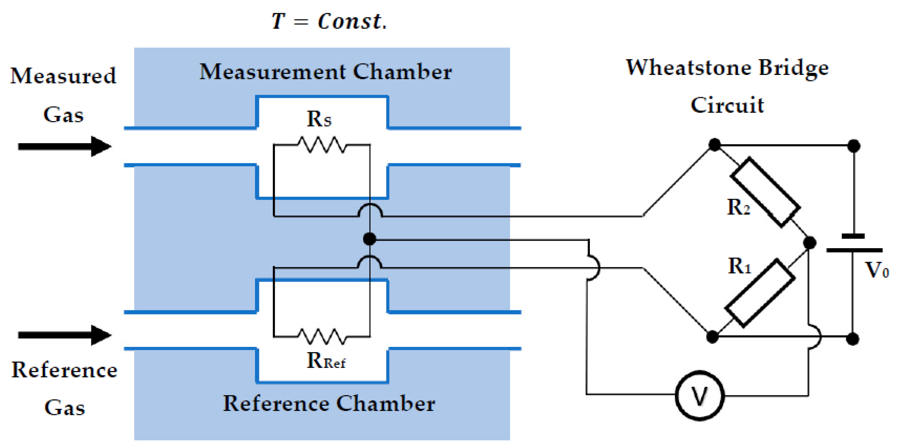
2.1.1. Thermal Conductivity Detector (TCD)
2.1.2. Thermal Conductivity Pellistor
2.2. Transient Operation
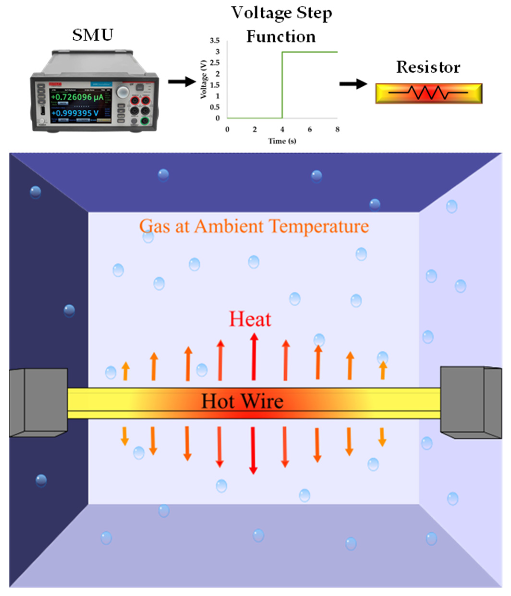
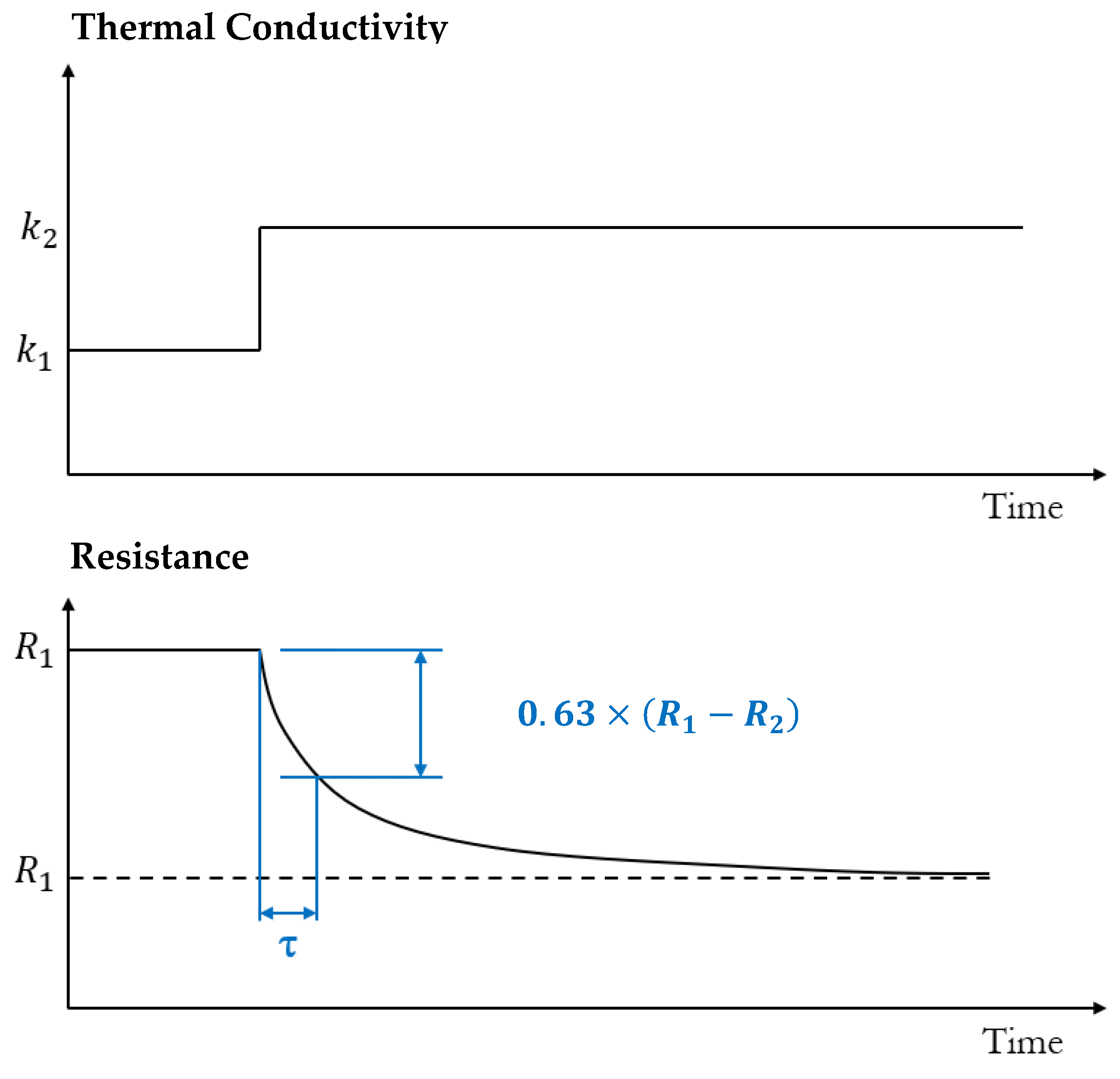
2.2.1. Transient Hot Wire Method (THM)
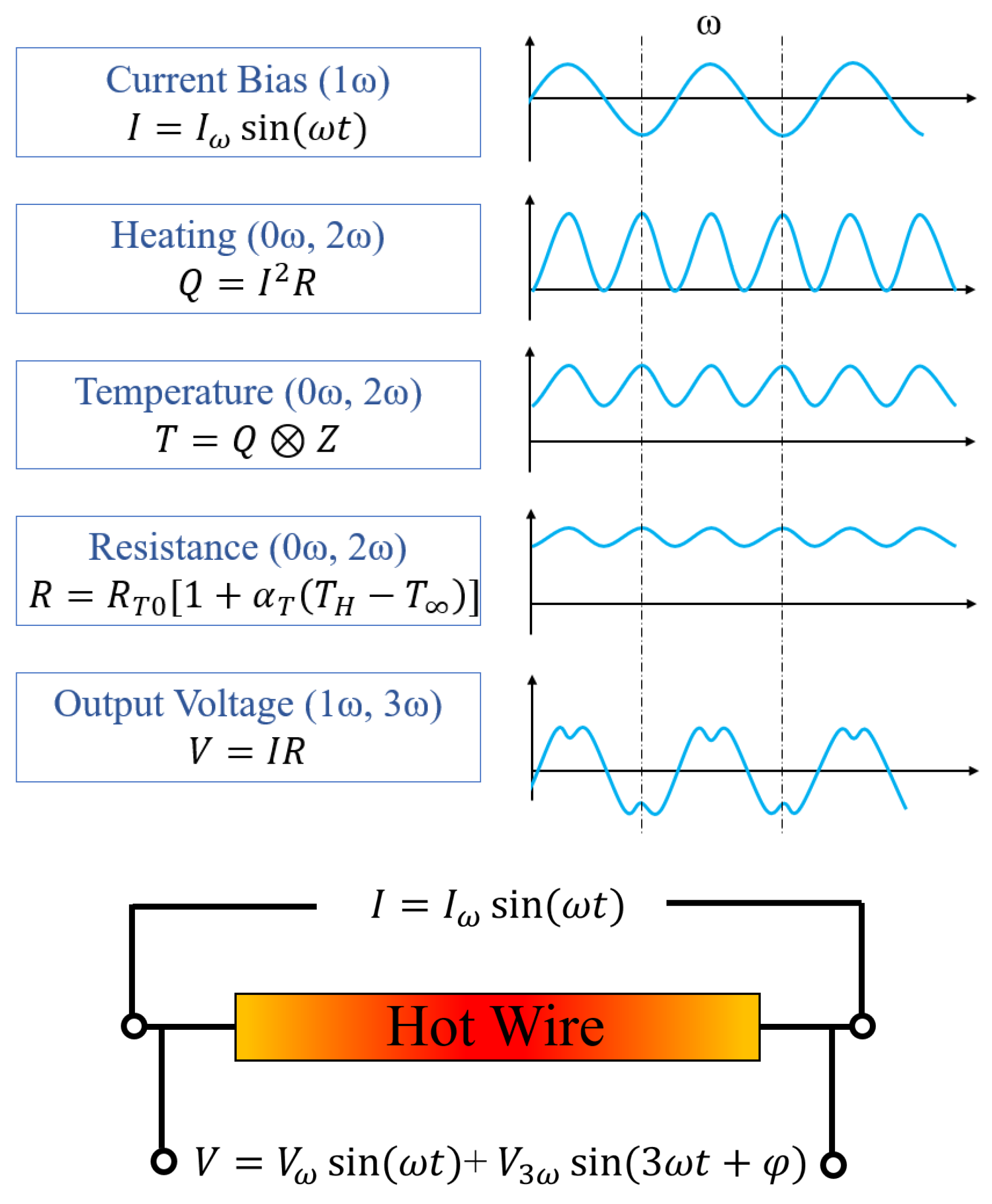
2.2.2. 3-Omega Method
2.2.3. Thermal Resonant
3. Signal Processing
3.1. Thermal Transduction Methods
3.1.1. Thermo-Resistive
3.1.2. Thermo-Electronic
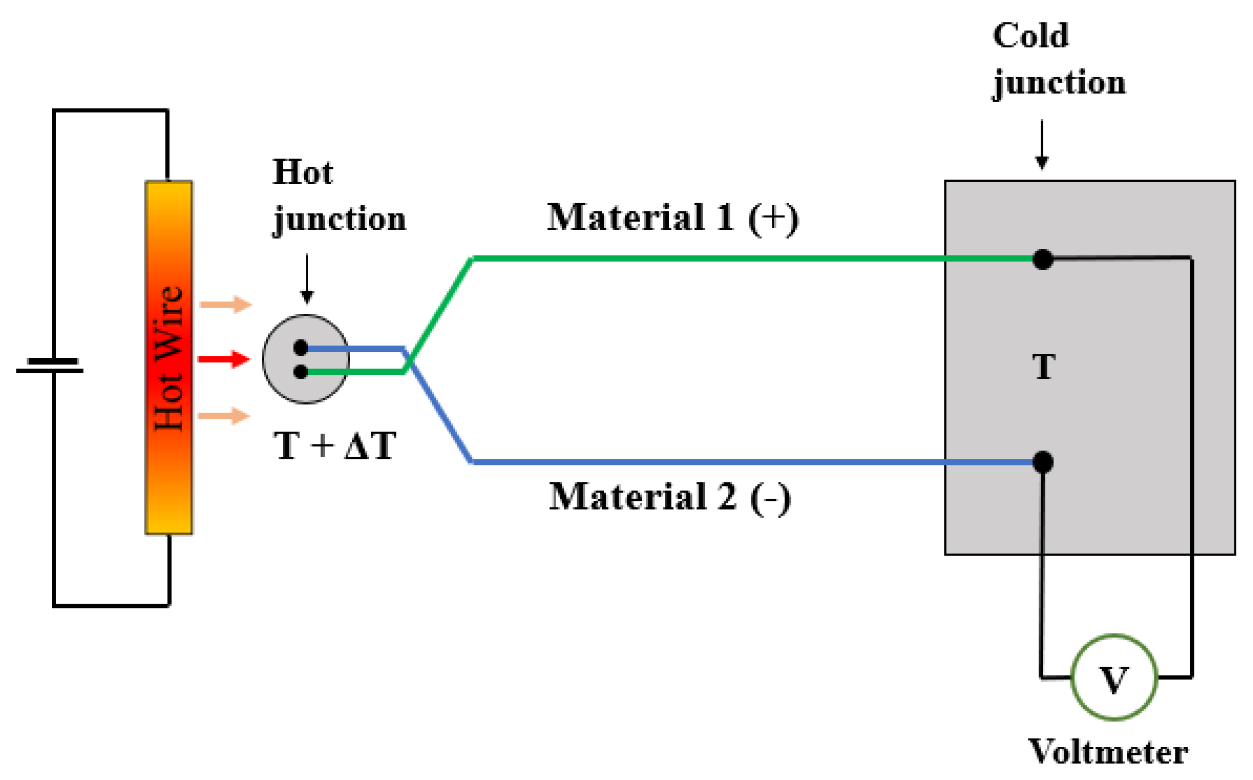
3.1.3. Thermo-Electric
4. Parasitics and Interference
4.1. Temperature
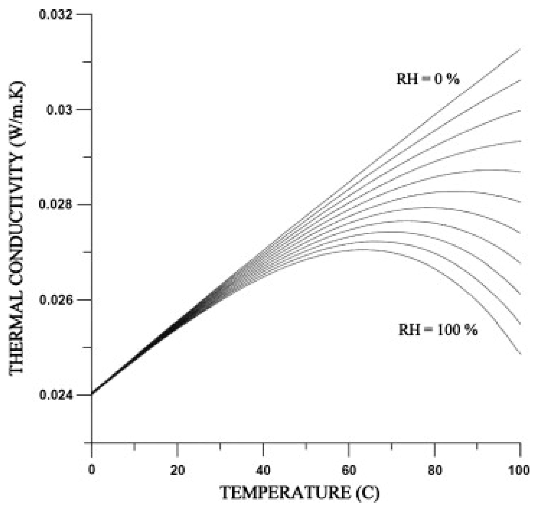
4.2. Humidity
- Condensed water droplets will not damage the sensor itself, or cause accelerated aging of the device.
- If there is potential for condensation in a system, there must be a method of purging or removing this condensation.
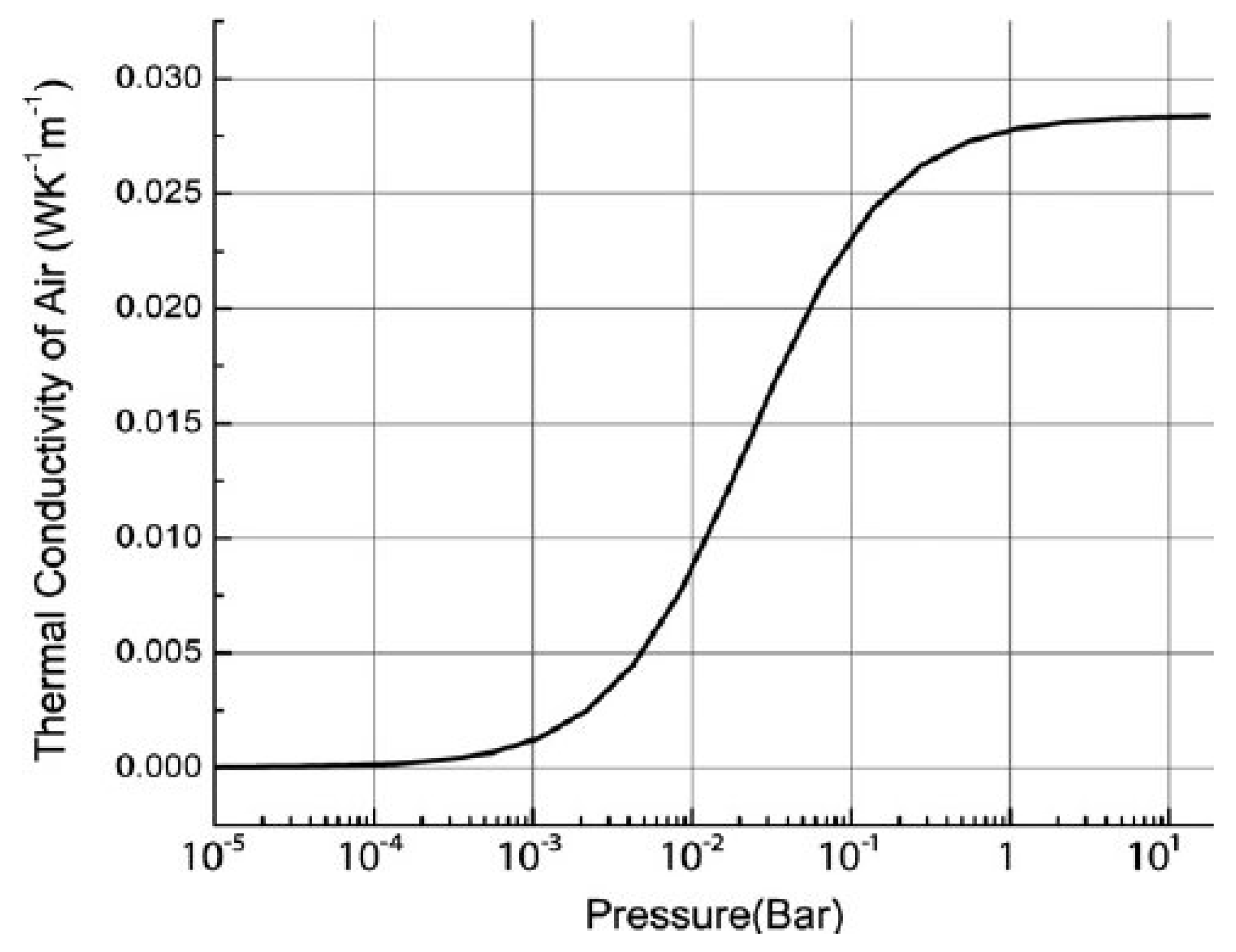
4.3. Pressure
4.4. Flow
4.5. Gas Mixtures
5. Applications
5.1. Gas Chromatography
5.2. Flammable Gas Sensing
5.3. Medical
5.4. Other
6. Recent Developments
6.1. Steady-State Operation
6.2. Transient Operation
6.2.1. Transient Hot Wire Method (and Other Temperature Modulation Techniques)
6.2.2. 3-Omega Method
6.3. Recent Developments Summary
7. Conclusions
8. Prospects
8.1. Sensitivity
8.2. Selectivity
8.3. Manufacturability and Integration
8.4. New Emerging Materials
8.5. Temperature Modulation
8.6. Artificial Intelligence
Author Contributions
Funding
Conflicts of Interest
References
- Gas Sensor Market Size & Share Report, 2022–2030. Available online: https://www.grandviewresearch.com/industry-analysis/gas-sensors-market (accessed on 21 October 2022).
- MEMS Sensor Market Size, Share|Vendors Analysis & Forecast. 2026. Available online: https://www.alliedmarketresearch.com/microelectromechanical-system-sensor-market (accessed on 21 October 2022).
- Nazemi, H.; Joseph, A.; Park, J.; Emadi, A. Advanced micro-and nano-gas sensor technology: A review. Sensors 2019, 19, 1285. [Google Scholar] [CrossRef] [PubMed]
- Niu, G.; Wang, F. A review of MEMS-based metal oxide semiconductors gas sensor in Mainland China. J. Micromech. Microeng. 2022, 32, 054003. [Google Scholar] [CrossRef]
- Gardner, E.L.; De Luca, A.; Vincent, T.; Jones, R.G.; Gardner, J.W.; Udrea, F. Thermal Conductivity Sensor with Isolating Membrane Holes. In Proceedings of the 2019 IEEE SENSORS, Montreal, QC, Canada, 27–30 October 2019; IEEE: Piscataway, NJ, USA, 2019; pp. 1–4. [Google Scholar]
- Daynes, H.A. Gas Analysis by Measurement of Thermal Conductivity; FOA: Rome, Italy, 1933. [Google Scholar]
- Szulczyński, B.; Gębicki, J. Currently commercially available chemical sensors employed for detection of volatile organic compounds in outdoor and indoor air. Environments 2017, 4, 21. [Google Scholar] [CrossRef]
- Wakeham, W.A. Measurement of the Transport Properties of Fluids; Experimental Thermodynamics Series; Stanford University: Stanford, CA, USA, 1991. [Google Scholar]
- Assael, M.J.; Antoniadis, K.D.; Metaxa, I.N.; Mylona, S.K.; Assael, J.-A.M.; Wu, J.; Hu, M. A novel portable absolute transient hot-wire instrument for the measurement of the thermal conductivity of solids. Int. J. Thermophys. 2015, 36, 3083–3105. [Google Scholar] [CrossRef]
- Assael, M.J.; Chen, C.-F.; Metaxa, I.; Wakeham, W.A. Thermal conductivity of suspensions of carbon nanotubes in water. Int. J. Thermophys. 2004, 25, 971–985. [Google Scholar] [CrossRef]
- Mylona, S.K.; Hughes, T.J.; Saeed, A.A.; Rowland, D.; Park, J.; Tsuji, T.; Tanaka, Y.; Seiki, Y.; May, E.F. Thermal conductivity data for refrigerant mixtures containing R1234yf and R1234ze (E). J. Chem. Thermodyn. 2019, 133, 135–142. [Google Scholar] [CrossRef]
- Healy, J.J.; De Groot, J.J.; Kestin, J. The theory of the transient hot-wire method for measuring thermal conductivity. Phys. B C 1976, 82, 392–408. [Google Scholar] [CrossRef]
- Corbino, O.M. Measurement of specific heats of metals at high temperatures. Atti Della R. Accad. Naz. Dei Lincei 1912, 21, 181–188. [Google Scholar]
- Birge, N.O.; Nagel, S.R. Wide-frequency specific heat spectrometer. Rev. Sci. Instrum. 1987, 58, 1464–1470. [Google Scholar] [CrossRef]
- Moon, I.K.; Jeong, Y.H.; Kwun, S.I. The 3Ω technique for measuring dynamic specific heat and thermal conductivity of a liquid or solid. Rev. Sci. Instrum. 1996, 67, 29–35. [Google Scholar] [CrossRef]
- Cahill, D.G.; Pohl, R.O. Thermal conductivity of amorphous solids above the plateau. Phys. Rev. B 1987, 35, 4067–4073. [Google Scholar] [CrossRef]
- Cahill, D.G. Thermal conductivity measurement from 30 to 750 K: The 3Ω method. Rev. Sci. Instrum. 1990, 61, 802–808. [Google Scholar] [CrossRef]
- Lee, S.-M.; Cahill, D.G. Heat transport in thin dielectric films. J. Appl. Phys. 1997, 81, 2590–2595. [Google Scholar] [CrossRef]
- Gesele, G.; Linsmeier, J.; Drach, V.; Fricke, J.; Arens-Fischer, R. Temperature-dependent thermal conductivity of porous silicon. J. Phys. Appl. Phys. 1997, 30, 2911–2916. [Google Scholar] [CrossRef]
- Hu, X.J.; Padilla, A.A.; Xu, J.; Fisher, T.S.; Goodson, K.E. 3-omega measurements of vertically oriented carbon nanotubes on silicon. J. Heat Transf. 2006, 128, 1109–1113. [Google Scholar] [CrossRef]
- Makarova, E.S.; Novotelnova, A.V. Estimating the uncertainty of measurements of thermal conductivity of thin films of thermoelectrics with the 3-omega method. J. Phys. Conf. Ser. 2021, 2057, 012108. [Google Scholar] [CrossRef]
- Bogner, M. Thermal Conductivity Measurements of Thin Films Using a Novel 3 Omega Method. Ph.D. Thesis, Northumbria University, Newcastle, UK, 2017. [Google Scholar]
- Cahill, D.G.; Ford, W.K.; Goodson, K.E.; Mahan, G.D.; Majumdar, A.; Maris, H.J.; Merlin, R.; Phillpot, S.R. Nanoscale thermal transport. J. Appl. Phys. 2003, 93, 793–818. [Google Scholar] [CrossRef]
- Mingo, N.; Broido, D.A. Length dependence of carbon nanotube thermal conductivity and the “problem of long waves”. Nano Lett. 2005, 5, 1221–1225. [Google Scholar] [CrossRef]
- Banerjee, K.; Wu, G.; Igeta, M.; Amerasekera, A.; Majumdar, A.; Hu, C. Investigation of self-heating phenomenon in small geometry vias using scanning joule expansion microscopy. In Proceedings of the 1999 IEEE International Reliability Physics Symposium Proceedings. 37th Annual (Cat. No. 99CH36296), San Diego, CA, USA, 23–25 March 1999; IEEE: Piscataway, NJ, USA, 1999; pp. 297–302. [Google Scholar]
- Cahill, D.G.; Goodson, K.; Majumdar, A. Thermometry and thermal transport in micro/nanoscale solid-state devices and structures. J. Heat Transf. 2002, 124, 223–241. [Google Scholar] [CrossRef]
- Kommandur, S.; Mahdavifar, A.; Hesketh, P.J.; Yee, S. A microbridge heater for low power gas sensing based on the 3-Omega technique. Sens. Actuators Phys. 2015, 233, 231–238. [Google Scholar] [CrossRef]
- Thundat, T.; Wachter, E.A.; Sharp, S.L.; Warmack, R.J. Detection of mercury vapor using resonating microcantilevers. Appl. Phys. Lett. 1995, 66, 1695–1697. [Google Scholar] [CrossRef]
- Lai, Y.-T.; Kuo, J.-C.; Yang, Y.-J. A novel gas sensor using polymer-dispersed liquid crystal doped with carbon nanotubes. Sens. Actuators Phys. 2014, 215, 83–88. [Google Scholar] [CrossRef]
- Jaber, N.; Ilyas, S.; Shekhah, O.; Eddaoudi, M.; Younis, M.I. Multimode excitation of a metal organics frameworks coated microbeam for smart gas sensing and actuation. Sens. Actuators Phys. 2018, 283, 254–262. [Google Scholar] [CrossRef]
- Waggoner, P.S.; Craighead, H.G. Micro-and nanomechanical sensors for environmental, chemical, and biological detection. Lab. Chip 2007, 7, 1238–1255. [Google Scholar] [CrossRef] [PubMed]
- Hajjaj, A.Z.; Jaber, N.; Alcheikh, N.; Younis, M.I. A sensitive resonant gas sensor based on multimode excitation of a buckled beam. In Proceedings of the 2019 20th International Conference on Solid-State Sensors, Actuators and Microsystems & Eurosensors XXXIII (TRANSDUCERS & EUROSENSORS XXXIII), Berlin, Germany, 23–27 June 2019; IEEE: Piscataway, NJ, USA, 2019; pp. 769–772. [Google Scholar]
- Harris, H. Concerning a thermometer with solid-state diodes. Sci. Am. 1961, 204, 192. [Google Scholar]
- McNamara, A.G. Semiconductor diodes and transistors as electrical thermometers. Rev. Sci. Instrum. 1962, 33, 330–333. [Google Scholar] [CrossRef]
- Mansoor, M.; Haneef, I.; Akhtar, S.; De Luca, A.; Udrea, F. Silicon diode temperature sensors—A review of applications. Sens. Actuators Phys. 2015, 232, 63–74. [Google Scholar] [CrossRef]
- Meijer, G.C. Thermal sensors based on transistors. Sens. Actuators 1986, 10, 103–125. [Google Scholar] [CrossRef]
- Kliche, K.; Billat, S.; Hedrich, F.; Ziegler, C.; Zengerle, R. Sensor for gas analysis based on thermal conductivity, specific heat capacity and thermal diffusivity. In Proceedings of the 2011 IEEE 24th International Conference on Micro Electro Mechanical Systems, Cancun, Mexico, 23–27 January 2011; IEEE: Piscataway, NJ, USA, 2011; pp. 1189–1192. [Google Scholar]
- De Graaf, G.; Abarca, A.; Ghaderi, M.; Wolffenbuttel, R.F. A MEMS flow compensated thermal conductivity detector for gas sensing. Procedia Eng. 2015, 120, 1265–1268. [Google Scholar] [CrossRef]
- Rastrello, F.; Placidi, P.; Scorzoni, A.; Cozzani, E.; Messina, M.; Elmi, I.; Zampolli, S.; Cardinali, G.C. Thermal Conductivity Detector for Gas Chromatography: Very Wide Gain Range Acquisition System and Experimental Measurements. IEEE Trans. Instrum. Meas. 2013, 62, 974–981. [Google Scholar] [CrossRef]
- Kaanta, B.C.; Chen, H.; Lambertus, G.; Steinecker, W.H.; Zhdaneev, O.; Zhang, X. High Sensitivity Micro-Thermal Conductivity Detector for Gas Chromatography. In Proceedings of the 2009 IEEE 22nd International Conference on Micro Electro Mechanical Systems, Sorrento, Italy, 25–29 January 2009; pp. 264–267. [Google Scholar]
- Kaanta, B.C.; Chen, H.; Zhang, X. A monolithically fabricated gas chromatography separation column with an integrated high sensitivity thermal conductivity detector. J. Micromech. Microeng. 2010, 20, 055016. [Google Scholar] [CrossRef]
- van der Bent, J.F.; Puik, E.; Tong, H.D.; van Rijn, C.J.M. Temperature balanced hydrogen sensor system with coupled palladium nanowires. Sens. Actuators Phys. 2015, 226, 98–106. [Google Scholar] [CrossRef]
- Zhang, H.; Shen, B.; Hu, W.; Liu, X. Research on a Fast-Response Thermal Conductivity Sensor Based on Carbon Nanotube Modification. Sensors 2018, 18, 2191. [Google Scholar] [CrossRef] [PubMed]
- Sun, X.; Ding, X.; Chen, Y.; He, G.; Bao, L. Temperature drift and compensation techniques for the thermal conductivity Gas sensor. In Proceedings of the Ifost, Ulaanbaatar, Mongolia, 28 June–1 July 2013; Volume 2, pp. 32–35. [Google Scholar]
- Gardner, E.L.W.; De Luca, A.; Udrea, F. Differential Thermal Conductivity CO2 Sensor. In Proceedings of the 2021 IEEE 34th International Conference on Micro Electro Mechanical Systems (MEMS), Gainesville, FL, USA, 25–29 January 2021; pp. 791–794. [Google Scholar]
- Tsilingiris, P.T. Thermophysical and transport properties of humid air at temperature range between 0 and 100°C. Energy Convers. Manag. 2008, 49, 1098–1110. [Google Scholar] [CrossRef]
- Simon, I.; Arndt, M. Thermal and gas-sensing properties of a micromachined thermal conductivity sensor for the detection of hydrogen in automotive applications. Sens. Actuators Phys. 2002, 97, 104–108. [Google Scholar] [CrossRef]
- Arndt, M. Micromachined thermal conductivity hydrogen detector for automotive applications. In Proceedings of the 2002 IEEE SENSORS, Orlando, FL, USA, 12–14 June 2002; Volume 2, pp. 1571–1575. [Google Scholar]
- Wu, H.; Grabarnik, S.; Emadi, A.; de Graaf, G.; Wolffenbuttel, R.F. Characterization of thermal cross-talk in a MEMS-based thermopile detector array. J. Micromech. Microeng. 2009, 19, 074022. [Google Scholar] [CrossRef]
- Kuo, J.T.; Yu, L.; Meng, E. Micromachined thermal flow sensors—A review. Micromachines 2012, 3, 550–573. [Google Scholar] [CrossRef]
- de Graaf, G.; Prouza, A.A.; Ghaderi, M.; Wolffenbuttel, R.F. Micro thermal conductivity detector with flow compensation using a dual MEMS device. Sens. Actuators Phys. 2016, 249, 186–198. [Google Scholar] [CrossRef]
- Hepp, C.J.; Krogmann, F.T.; Urban, G.A. Flow rate independent sensing of thermal conductivity in a gas stream by a thermal MEMS-sensor–Simulation and experiments. Sens. Actuators Phys. 2017, 253, 136–145. [Google Scholar] [CrossRef]
- Romero, D.F.R.; Kogan, K.; Cubukcu, A.S.; Urban, G.A. Simultaneous flow and thermal conductivity measurement of gases utilizing a calorimetric flow sensor. Sens. Actuators Phys. 2013, 203, 225–233. [Google Scholar] [CrossRef]
- Wang, J.; Liu, Y.; Zhou, H.; Wang, Y.; Wu, M.; Huang, G.; Li, T. Thermal Conductivity Gas Sensor with Enhanced Flow-Rate Independence. Sensors 2022, 22, 1308. [Google Scholar] [CrossRef] [PubMed]
- Cheung, H.; Bromley, L.A.; Wilke, C.R. Thermal conductivity of gas mixtures. AIChE J. 1962, 8, 221–228. [Google Scholar] [CrossRef]
- Brokaw, R.S. Approximate formulas for the viscosity and thermal conductivity of gas mixtures. J. Chem. Phys. 1958, 29, 391–397. [Google Scholar] [CrossRef]
- Lindsay, A.L.; Bromley, L.A. Thermal conductivity of gas mixtures. Ind. Eng. Chem. 1950, 42, 1508–1511. [Google Scholar] [CrossRef]
- Mason, E.A.; Saxena, S.C. Approximate formula for the thermal conductivity of gas mixtures. Phys. Fluids 1958, 1, 361–369. [Google Scholar] [CrossRef]
- Monchick, L.; Pereira, A.N.G.; Mason, E.A. Heat conductivity of polyatomic and polar gases and gas mixtures. J. Chem. Phys. 1965, 42, 3241–3256. [Google Scholar] [CrossRef]
- Zhukov, V.P.; Pätz, M. On thermal conductivity of gas mixtures containing hydrogen. Heat Mass Transf. 2017, 53, 2219–2222. [Google Scholar] [CrossRef]
- Azmi, W.H.; Sharma, K.V.; Mamat, R.; Najafi, G.; Mohamad, M.S. The enhancement of effective thermal conductivity and effective dynamic viscosity of nanofluids–A review. Renew. Sustain. Energy Rev. 2016, 53, 1046–1058. [Google Scholar] [CrossRef]
- Terry, S.C.; Jerman, J.H.; Angell, J.B. A gas chromatographic air analyzer fabricated on a silicon wafer. IEEE Trans. Electron Devices 1979, 26, 1880–1886. [Google Scholar] [CrossRef]
- Mahdavifar, A.; Aguilar, R.; Peng, Z.; Hesketh, P.J.; Findlay, M.; Stetter, J.R.; Hunter, G.W. Simulation and fabrication of an ultra-low power miniature microbridge thermal conductivity gas sensor. J. Electrochem. Soc. 2014, 161, B55–B61. [Google Scholar] [CrossRef]
- Mahdavifar, A.; Navaei, M.; Hesketh, P.J.; Findlay, M.; Stetter, J.R.; Hunter, G.W. Transient thermal response of micro-thermal conductivity detector (µTCD) for the identification of gas mixtures: An ultra-fast and low power method. Microsyst. Nanoeng. 2015, 1, 15025. [Google Scholar] [CrossRef]
- Narayanan, S.; Agah, M. A high-performance TCD monolithically integrated with a gas separation column. In Proceedings of the 2012 IEEE SENSORS, Taipei, Taiwan, 28–31 October 2012; pp. 1–4. [Google Scholar]
- Narayanan, S.; Alfeeli, B.; Agah, M. Two-Port Static Coated Micro Gas Chromatography Column With an Embedded Thermal Conductivity Detector. IEEE Sens. J. 2012, 12, 1893–1900. [Google Scholar] [CrossRef]
- Legendre, O.; Ruellan, J.; Gely, M.; Arcamone, J.; Duraffourg, L.; Ricoul, F.; Alava, T.; Fain, B. CMOS compatible nanoscale thermal conductivity detector for gas sensing applications. Sens. Actuators Phys. 2017, 261, 9–13. [Google Scholar] [CrossRef]
- Cruz, D.; Chang, J.P.; Showalter, S.K.; Gelbard, F.; Manginell, R.P.; Blain, M.G. Microfabricated thermal conductivity detector for the micro-ChemLabTM. Sens. Actuators B Chem. 2007, 121, 414–422. [Google Scholar] [CrossRef]
- Sun, J.; Cui, D.; Chen, X.; Zhang, L.; Cai, H.; Li, H. Design, modeling, microfabrication and characterization of novel micro thermal conductivity detector. Sens. Actuators B Chem. 2011, 160, 936–941. [Google Scholar] [CrossRef]
- Garg, A.; Akbar, M.; Vejerano, E.; Narayanan, S.; Nazhandali, L.; Marr, L.C.; Agah, M. Zebra GC: A mini gas chromatography system for trace-level determination of hazardous air pollutants. Sens. Actuators B Chem. 2015, 212, 145–154. [Google Scholar] [CrossRef]
- Qu, H.; Duan, X. Recent advances in micro detectors for micro gas chromatography. Sci. China Mater. 2019, 62, 611–623. [Google Scholar] [CrossRef]
- Palmisano, V.; Boon-Brett, L.; Bonato, C.; Harskamp, F.; Buttner, W.J.; Post, M.B.; Burgess, R.; Rivkin, C. Evaluation of selectivity of commercial hydrogen sensors. Int. J. Hydrogen Energy 2014, 39, 20491–20496. [Google Scholar] [CrossRef]
- Buttner, W.J.; Post, M.B.; Burgess, R.; Rivkin, C. An overview of hydrogen safety sensors and requirements. Int. J. Hydrogen Energy 2011, 36, 2462–2470. [Google Scholar] [CrossRef]
- Harkinezhad, B.; Soleimani, A.; Hossein-Babaei, F. Hydrogen level detection via thermal conductivity measurement using temporal temperature monitoring. In Proceedings of the 2019 27th Iranian Conference on Electrical Engineering (ICEE), Yazd, Iran, 30 April–2 May 2019; IEEE: Piscataway, NJ, USA, 2019; pp. 408–411. [Google Scholar]
- Steckelmacher, W.; Tinsley, D.M. Thermal conductivity leak detectors suitable for testing equipment by overpressure or vacuum. Vacuum 1962, 12, 153–159. [Google Scholar] [CrossRef]
- Boon-Brett, L.; Bousek, J.; Moretto, P. Reliability of commercially available hydrogen sensors for detection of hydrogen at critical concentrations: Part II–selected sensor test results. Int. J. Hydrogen Energy 2009, 34, 562–571. [Google Scholar] [CrossRef]
- Berndt, D.; Muggli, J.; Wittwer, F.; Langer, C.; Heinrich, S.; Knittel, T.; Schreiner, R. MEMS-based thermal conductivity sensor for hydrogen gas detection in automotive applications. Sens. Actuators Phys. 2020, 305, 111670. [Google Scholar] [CrossRef]
- Pollak-Diener, G.; Obermeier, E. Heat-conduction microsensor based on silicon technology for the analysis of two-and three-component gas mixtures. Sens. Actuators B Chem. 1993, 13, 345–347. [Google Scholar] [CrossRef]
- Ma, H.; Qin, S.; Wang, L.; Wang, G.; Zhao, X.; Ding, E. The study on methane sensing with high-temperature low-power CMOS compatible silicon microheater. Sens. Actuators B Chem. 2017, 244, 17–23. [Google Scholar] [CrossRef]
- Puente, D.; Gracia, F.J.; Ayerdi, I. Thermal conductivity microsensor for determining the Methane Number of natural gas. Sens. Actuators B Chem. 2005, 110, 181–189. [Google Scholar] [CrossRef]
- Dent, A.G.; Sutedja, T.G.; Zimmerman, P.V. Exhaled breath analysis for lung cancer. J. Thorac. Dis. 2013, 5, S540–S550. [Google Scholar]
- Ohira, S.-I.; Toda, K. Micro gas analyzers for environmental and medical applications. Anal. Chim. Acta 2008, 619, 143–156. [Google Scholar] [CrossRef]
- Righettoni, M.; Tricoli, A.; Pratsinis, S.E. Si: WO3 sensors for highly selective detection of acetone for easy diagnosis of diabetes by breath analysis. Anal. Chem. 2010, 82, 3581–3587. [Google Scholar] [CrossRef]
- Liu, S.-J.; Chen, Z.-Y.; Chang, Y.-Z.; Wang, S.-L.; Li, Q.; Fan, Y.-Q. Xenon Responding Analyzed by Using Micro-Thermal Conductivity Detector for Gas Chromatography. Fenxi Huaxue 2012, 40, 1130–1134. [Google Scholar] [CrossRef]
- Luginbühl, M.; Lauber, R.; Feigenwinter, P.; Zbinden, A.M. Monitoring xenon in the breathing circuit with a thermal conductivity sensor. J. Clin. Monit. Comput. 2002, 17, 23–30. [Google Scholar] [CrossRef]
- Houston, T.E. Methods for the determination of water in coatings. Met. Finish. 1997, 95, 36–38. [Google Scholar] [CrossRef]
- Nussbaum, R.; Lischke, D.; Paxmann, H.; Wolf, B. Quantitative GC determination of water in small samples. Chromatographia 2000, 51, 119–121. [Google Scholar] [CrossRef]
- O’Keefe, W.K.; Ng, F.T.T.; Rempel, G.L. Validation of a gas chromatography/thermal conductivity detection method for the determination of the water content of oxygenated solvents. J. Chromatogr. A 2008, 1182, 113–118. [Google Scholar] [CrossRef] [PubMed]
- Weatherly, C.A.; Woods, R.M.; Armstrong, D.W. Rapid analysis of ethanol and water in commercial products using ionic liquid capillary gas chromatography with thermal conductivity detection and/or barrier discharge ionization detection. J. Agric. Food Chem. 2014, 62, 1832–1838. [Google Scholar] [CrossRef] [PubMed]
- Wilfert, S.; Edelmann, C. Miniaturized vacuum gauges. J. Vac. Sci. Technol. Vac. Surf. Films 2004, 22, 309–320. [Google Scholar] [CrossRef]
- Kerkeni, C.; BenJemaa, F.; Kooli, S.; Farhat, A.; Maalej, M. Performance evaluation of a thermodynamic solar power plant: Fifteen years of operation history. Renew. Energy 2002, 25, 473–487. [Google Scholar] [CrossRef]
- Van Herwaarden, A.W.; Sarro, P.M.; Meijer, H.C. Integrated vacuum sensor. Sens. Actuators 1985, 8, 187–196. [Google Scholar] [CrossRef]
- Paul, O.; Brand, O.; Lenggenhager, R.; Baltes, H. Vacuum gauging with complementary metal–oxide–semiconductor microsensors. J. Vac. Sci. Technol. Vac. Surf. Films 1995, 13, 503–508. [Google Scholar] [CrossRef]
- Paul, O.; Haberli, A.; Malcovati, P.; Baltes, H. Novel integrated thermal pressure gauge and read-out circuit by CMOS IC technology. In Proceedings of the 1994 IEEE International Electron Devices Meeting, San Francisco, CA, USA, 11–14 December 1994; IEEE: Piscataway, NJ, USA, 1994; pp. 131–134. [Google Scholar]
- Mastrangelo, C.H.; Muller, R.S. Microfabricated thermal absolute-pressure sensor with on-chip digital front-end processor. IEEE J. Solid-State Circuits 1991, 26, 1998–2007. [Google Scholar] [CrossRef]
- Wang, J.; Tang, Z.; Li, J. Tungsten-microhotplate-array-based pirani vacuum sensor system with on-chip digital front-end processor. J. Microelectromech. Syst. 2011, 20, 834–841. [Google Scholar] [CrossRef]
- Piotto, M.; Del Cesta, S.; Bruschi, P. A CMOS compatible micro-Pirani vacuum sensor based on mutual heat transfer with 5-decade operating range and 0.3 Pa detection limit. Sens. Actuators Phys. 2017, 263, 718–726. [Google Scholar] [CrossRef]
- Stark, B.H.; Najafi, K. A low-temperature thin-film electroplated metal vacuum package. J. Microelectromech. Syst. 2004, 13, 147–157. [Google Scholar] [CrossRef]
- Topalli, E.S.; Topalli, K.; Alper, S.E.; Serin, T.; Akin, T. Pirani vacuum gauges using silicon-on-glass and dissolved-wafer processes for the characterization of MEMS vacuum packaging. IEEE Sens. J. 2009, 9, 263–270. [Google Scholar] [CrossRef]
- Feng, F.; Tian, B.; Hou, L.; Yu, Z.; Zhou, H.; Ge, X.; Li, X. High sensitive micro thermal conductivity detector with sandwich structure. In Proceedings of the 2017 19th International Conference on Solid-State Sensors, Actuators and Microsystems (TRANSDUCERS), Kaohsiung, Taiwan, 18–22 June 2017; 2017; pp. 1433–1436. [Google Scholar]
- Wang, J.Q.; Tang, Z.A. A CMOS-compatible temperature sensor based on the gaseous thermal conduction dependent on temperature. Sens. Actuators Phys. 2012, 176, 72–77. [Google Scholar] [CrossRef]
- Sarfraz, S.; Kumar, R.V.; Udrea, F. A high temperature and low power SOI CMOS MEMS based thermal conductivity gas sensor. In Proceedings of the CAS 2013 (International Semiconductor Conference), Sinaia, Romania, 14–16 October 2013; Volume 1, pp. 51–54. [Google Scholar]
- Struk, D.; Shirke, A.; Mahdavifar, A.; Hesketh, P.J.; Stetter, J.R. Investigating time-resolved response of micro thermal conductivity sensor under various modes of operation. Sens. Actuators B Chem. 2018, 254, 771–777. [Google Scholar] [CrossRef]
- Kawano, T.; Chiamori, H.C.; Suter, M.; Zhou, Q.; Sosnowchik, B.D.; Lin, L. An Electrothermal Carbon Nanotube Gas Sensor. Nano Lett. 2007, 7, 3686–3690. [Google Scholar] [CrossRef] [PubMed]
- Zou, Z.; Zhang, H.; Sun, Y.; Gao, Y.; Dou, L. A thermal conductivity sensor based on mixed carbon material modification for hydrogen detection. Rev. Sci. Instrum. 2022, 93, 035001. [Google Scholar] [CrossRef]
- Cho, W.; Kim, T.; Shin, H. Thermal conductivity detector (TCD)-type gas sensor based on a batch-fabricated 1D nanoheater for ultra-low power consumption. Sens. Actuators B Chem. 2022, 371, 132541. [Google Scholar] [CrossRef]
- Sosna, C.; Buchner, R.; Lang, W. A temperature compensation circuit for thermal flow sensors operated in constant-temperature-difference mode. IEEE Trans. Instrum. Meas. 2010, 59, 1715–1721. [Google Scholar] [CrossRef]
- Ferreira, R.P.C.; Freire, R.C.S.; Deep, C.S.; de Rocha Neto, J.S.; Oliveira, A. Hot-wire anemometer with temperature compensation using only one sensor. IEEE Trans. Instrum. Meas. 2001, 50, 954–958. [Google Scholar] [CrossRef]
- Kielbasa, J.; Ligeza, P. Temperature-compensated single hot-wire anemometer. In Tagung Turbulente Ein-und Mehrphasenstrmungen; Institut für Mechanik: Darmstadt, Germany, 1991; pp. 75–86. [Google Scholar]
- Xu, W.; Gao, B.; Ma, S.; Zhang, A.; Chiu, Y.; Lee, Y.-K. Low-cost temperature-compensated thermoresistive micro calorimetric flow sensor by using 0.35 μm CMOS MEMS technology. In Proceedings of the 2016 IEEE 29th International Conference on Micro Electro Mechanical Systems (MEMS), Shanghai, China, 24–28 January 2016; IEEE: Piscataway, NJ, USA, 2016; pp. 189–192. [Google Scholar]
- Cai, Z.; van Veldhoven, R.H.M.; Falepin, A.; Suy, H.; Sterckx, E.; Bitterlich, C.; Makinwa, K.A.A.; Pertijs, M.A.P. A Ratiometric Readout Circuit for Thermal-Conductivity-Based Resistive CO2 Sensors. IEEE J. Solid-State Circuits 2016, 51, 2463–2474. [Google Scholar] [CrossRef]
- Ali, H.A.; Pirro, M.; Poulichet, P.; CESAR, W.; Marty, F.; AZZOUZ, I.; Gnambodoe-Capochichi, M.; Nefzaoui, E.; Bourouina, T. Thermal aspects of a micro thermal conductivity detector for micro gas chromatography. In Proceedings of the 2019 Symposium on Design, Test, Integration & Packaging of MEMS and MOEMS (DTIP), Paris, France, 12–15 May 2019; IEEE: Paris, France, 2019; pp. 1–6. [Google Scholar]
- Udina, S.; Carmona, M.; Carles, G.; Santander, J.; Fonseca, L.; Marco, S. A micromachined thermoelectric sensor for natural gas analysis: Thermal model and experimental results. Sens. Actuators B Chem. 2008, 134, 551–558. [Google Scholar] [CrossRef]
- Gardner, E.L.; Vincent, T.A.; De Luca, A.; Udrea, F. Simultaneous Flow and Thermal Conductivity Sensing on a Single Chip Using Artificial Neural Networks. IEEE Sens. J. 2020, 20, 4985–4991. [Google Scholar] [CrossRef]
- Randjelović, D.V. Analytical Modelling Approach in Study of the Transient Response of Thermopile-Based MEMS Sensors Applied for Simultaneous Detection of Pressure and Gas Composition. In Proceedings of the 2018 International Semiconductor Conference (CAS), Sinaia, Romania, 10–12 October 2018; pp. 27–34. [Google Scholar]
- Cai, Z.; van Veldhoven, R.; Suy, H.; de Graaf, G.; Makinwa, K.A.A.; Pertijs, M.A.P. A Phase-Domain Readout Circuit for a CMOS-Compatible Hot-Wire CO2 Sensor. IEEE J. Solid-State Circuits 2018, 53, 3303–3313. [Google Scholar] [CrossRef]
- Sun, J.; Chen, T.; Tan, T.; Wang, D.; Zhu, X.; Zhang, X.; Peng, H.; Luan, Z. Fabrication and Characterization of a Novel Micro-Thermal Conductivity Detector for Monitoring Small-molecule Gases. IEEE Sens. J. 2020, 20, 11115–11121. [Google Scholar] [CrossRef]
- Harumoto, T.; Fujiki, H.; Shi, J.; Nakamura, Y. Extremely simple structure hydrogen gas sensor based on single metallic thin-wire under sweep heating. Int. J. Hydrogen Energy 2022, 47, 34291–34298. [Google Scholar] [CrossRef]
- Lotfi, A.; Navaei, M.; Hesketh, P.J. A Platinum Cantilever-Based TCD for 3-Omega Sensing of Gas Mixtures. ECS Trans. 2018, 86, 79–86. [Google Scholar] [CrossRef]
- Lotfi, A.; Navaei, M.; Hesketh, P.J. A Platinum Cantilever-Based Thermal Conductivity Detector for Ammonia Sensing Using the 3-Omega Technique. ECS J. Solid State Sci. Technol. 2019, 8, Q126–Q133. [Google Scholar] [CrossRef]
- Lotfi, A.; Navaei, M.; Hesketh, P.J. Balanced Dual Platinum Micro-Cantilever Thermal Conductivity Gas Sensor Using 3-Omega Technique. ECS Meet. Abstr. 2021, MA2021-01, 1547. [Google Scholar] [CrossRef]
- Gardner, J.W.; Bartlett, P.N. Electronic Noses: Principles and Applications; Oxford University Press on Demand: Oxford, UK, 1999. [Google Scholar]
- Sadek, K.; Moussa, W. Assessment of the Effect of Micro-Fabrication Uncertainties on the Sensitivity of Gas Sensors Using 3-D Finite Element Modeling. In Proceedings of the 2004 International Conference on MEMS, NANO and Smart Systems (ICMENS’04), Banff, AB, Canada, 25–27 August 2004; IEEE: Piscataway, NJ, USA, 2004; pp. 663–665. [Google Scholar]
- Son, K.; Liao, A.; Lung, G.; Gallegos, M.; Hatake, T.; Harris, R.D.; Scheick, L.Z.; Smythe, W.D. GaN-based high temperature and radiation-hard electronics for harsh environments. Nanosci. Nanotechnol. Lett. 2010, 2, 89–95. [Google Scholar] [CrossRef]
- Lee, A.P.; Reedy, B.J. Temperature modulation in semiconductor gas sensing. Sens. Actuators B Chem. 1999, 60, 35–42. [Google Scholar] [CrossRef]
- Urasinska-Wojcik, B.; Gardner, J.W. Identification of H2S impurity in hydrogen using temperature modulated metal oxide resistive sensors with a novel signal processing technique. IEEE Sens. Lett. 2017, 1, 1–4. [Google Scholar] [CrossRef]
- Li, F.; Jin, H.; Wang, J.; Zou, J.; Jian, J. Selective sensing of gas mixture via a temperature modulation approach: New strategy for potentiometric gas sensor obtaining satisfactory discriminating features. Sensors 2017, 17, 573. [Google Scholar] [CrossRef] [PubMed]
- Durán, C.; Benjumea, J.; Carrillo, J. Response optimization of a chemical gas sensor array using temperature modulation. Electronics 2018, 7, 54. [Google Scholar] [CrossRef]
- Feng, S.; Farha, F.; Li, Q.; Wan, Y.; Xu, Y.; Zhang, T.; Ning, H. Review on smart gas sensing technology. Sensors 2019, 19, 3760. [Google Scholar] [CrossRef]


| Gas Type | Gas | Thermal Conductivity [10−3 W/m·K] | Specific Heat Capacity [J/(K·kg)] | Density [kg/m3] |
|---|---|---|---|---|
| Inert | Air | 26.2 | 1000 | 1.20 |
| Ar | 17.9 | 521.5 | 1.78 | |
| He | 156.7 | 5193.0 | 0.179 | |
| CO2 | 16.8 | 852.5 | 1.84 | |
| Ne | 49.8 | 1030 | 0.9 | |
| N2 | 26 | 1041.8 | 1.126 | |
| Toxic | CO | 25 | 1040 | 1.123 |
| NH3 | 24.4 | 2200 | 0.690 | |
| N2O | 17.4 | 880 | 1.98 | |
| H2S | 14.6 | 2240 | 1.36 | |
| Flammable | H2 | 186.9 | 14310 | 0.09 |
| CH4 | 34.1 | 2235.8 | 0.657 | |
| C4H10 | 16.4 | 1730 | 573 | |
| O2 | 26.3 | 918 | 1.43 | |
| Volatile Organic Compound (VOC) | C7H8 (Toluene) | 134 | 1130 | 862 |
| C3H6O (Acetone) | 11.5 | 1290 | 784.5 | |
| C2H6O (Ethanol) | 14.4 | 1600 | 785.3 | |
| CH2O (Formaldehyde) | - | - | 815 | |
| C8H10 (Xylene) | - | 1720 | 860 | |
| C6H6 (Benzene) | - | 1800 | 876 |
| Transduction Principle | Thermo-Resistive | Thermo-Electric | Thermo-Electronic |
|---|---|---|---|
| Example sensor | RTD Thermistor | Thermocouple Thermopile | Diode Transistor |
| Advantages | Cheap Good linearity High stability Can be suspended | Self-powered Wide temperature range Simple Accurate Fast response time | Linear Wide temperature range Low current No self-heating Small |
| Drawbacks | Current sourced Self-heating Electro-migration | Non-linear Low voltage Low stability Cold junction required | High thermal noise Large occupied area High resistance |
| Detector | Selectivity | LoD | Cost |
|---|---|---|---|
| Thermal Conductivity Detector (TCD) | Responds if thermal conductivity of gas is different to that of the carrier gas. | 1 ng/mL | Low |
| Flame Ionisation Detector (FID) | Organic compounds. | 1 pg(C)/s | Medium |
| Electron-Capture Detector (ECD) | Electron capturing compounds, such as halogens. | 10 fg/s | High |
| Electrolytic Conductivity Sensor (ELCD) | Halogens and S. | 1 pg CI/s | Medium |
| Atomic Emission Detector (AED) | Element selective. | 0.1–50 pg/s | High |
| Property (Units) | Al | W | Au | Pt |
|---|---|---|---|---|
| Electrical Conductivity (S/m) | 377 | 183 | 488 | 94 |
| Melting Point (°C) | 660 | 3410 | 1064 | 1772 |
| Density (kg/m3) | 2720 | 19,350 | 19,320 | 21,450 |
| TCR (10−4/°C) | 39 | 45 | 34 | 30 |
| Thermal Conductivity (W/m/K) | 236 | 177 | 319 | 72 |
| Specific Heat Capacity (J/K/kg) | 904 | 134 | 129 | 133 |
| Linear Expansivity (K−1) | 23.1 | 4.5 | 14.2 | 8.8 |
| Young’s Modulus (GPa) | 70 | 411 | 78 | 168 |
| Yield Strength (MPa) | 50 | 750 | 200 | <14 |
| Poisson’s Ratio | 0.35 | 0.28 | 0.44 | 0.38 |
| Reference | Operation | Measured Gas | Heater Material | Limit of Detection | Comments |
|---|---|---|---|---|---|
| [46] | Steady-state | Hydrogen | Platinum | 2000 ppm | Helium used in experiment |
| [105] | Steady-state | Helium | Carbon and gold | 142 ppm | Low power consumption of 240 nW using PWM |
| [110] | Steady-state | Carbon dioxide | Tungsten | 200 ppm | Ratiometric readout circuit |
| [4] | Steady-state | Tungsten | Tungsten | 100 ppm | Differential measurement on single membrane |
| [63] | Transient | Tungsten | Polysilicon | 178 ppm | Data obtained for other gases as well |
| [102] | Transient | Polysilicon | Polysilicon | 3313 ppm | Data obtained for other gases as well |
| [115] | Transient | Polysilicon | Tungsten | 94 ppm | Uses thermal time constants |
| [116] | Transient | Tungsten | Platinum | 5 ppm | Other gases investigated, GC system. |
| [117] | Transient | Platinum, tungsten and cobalt | Platinum, tungsten and cobalt | 10,000 ppm | Uses a temperature modulation method |
| [119] | Transient | Platinum | Platinum | 30 ppm | Cantilever based design. |
Disclaimer/Publisher’s Note: The statements, opinions and data contained in all publications are solely those of the individual author(s) and contributor(s) and not of MDPI and/or the editor(s). MDPI and/or the editor(s) disclaim responsibility for any injury to people or property resulting from any ideas, methods, instructions or products referred to in the content. |
© 2023 by the authors. Licensee MDPI, Basel, Switzerland. This article is an open access article distributed under the terms and conditions of the Creative Commons Attribution (CC BY) license (https://creativecommons.org/licenses/by/4.0/).
Share and Cite
Gardner, E.L.W.; Gardner, J.W.; Udrea, F. Micromachined Thermal Gas Sensors—A Review. Sensors 2023, 23, 681. https://doi.org/10.3390/s23020681
Gardner ELW, Gardner JW, Udrea F. Micromachined Thermal Gas Sensors—A Review. Sensors. 2023; 23(2):681. https://doi.org/10.3390/s23020681
Chicago/Turabian StyleGardner, Ethan L. W., Julian W. Gardner, and Florin Udrea. 2023. "Micromachined Thermal Gas Sensors—A Review" Sensors 23, no. 2: 681. https://doi.org/10.3390/s23020681
APA StyleGardner, E. L. W., Gardner, J. W., & Udrea, F. (2023). Micromachined Thermal Gas Sensors—A Review. Sensors, 23(2), 681. https://doi.org/10.3390/s23020681