Systematic Review

Continual Deep Learning for Time Series Modeling

1
International Association of Engineers, Unit 1, 1/F, Hung To Road, Hong Kong
2
School of Computing Technologies, RMIT University, Building 14, Melbourne, VIC 3000, Australia
*
Author to whom correspondence should be addressed.
Sensors 2023, 23(16), 7167; https://doi.org/10.3390/s23167167
Submission received: 12 June 2023 / Revised: 31 July 2023 / Accepted: 10 August 2023 / Published: 14 August 2023
(This article belongs to the Section Sensors Development)

Abstract

:
The multi-layer structures of Deep Learning facilitate the processing of higher-level abstractions from data, thus leading to improved generalization and widespread applications in diverse domains with various types of data. Each domain and data type presents its own set of challenges. Real-world time series data may have a non-stationary data distribution that may lead to Deep Learning models facing the problem of catastrophic forgetting, with the abrupt loss of previously learned knowledge. Continual learning is a paradigm of machine learning to handle situations when the stationarity of the datasets may no longer be true or required. This paper presents a systematic review of the recent Deep Learning applications of sensor time series, the need for advanced preprocessing techniques for some sensor environments, as well as the summaries of how to deploy Deep Learning in time series modeling while alleviating catastrophic forgetting with continual learning methods. The selected case studies cover a wide collection of various sensor time series applications and can illustrate how to deploy tailor-made Deep Learning, advanced preprocessing techniques, and continual learning algorithms from practical, real-world application aspects.

1. Introduction

Time series modeling is a challenging task in data mining and machine learning. Popular time series modeling tasks include classification, anomaly detection, regression, forecasting, and clustering. A time series is a sequence of measurements taken at various times. Spatial time series data refers to multiple time series data corresponding to different spatial locations. The spatial–temporal models face difficulties in addressing not only the short-term and long-term patterns but also the spatial patterns [1]. Time series datasets have the property of temporal ordering by nature [2]. Generally speaking, time series models have the capability to utilize the fact that observations closer together in time relate more closely. Time series modeling has many real-world applications like environment and traffic tasks, and successful modeling for the time series has become increasingly important. For example, wind time series forecasting is essential for the decision-making of electric system operators.
Time series analysis models can be divided broadly into time domain models and frequency domain models. The time domain model investigates the data with respect to time, while the frequency domain models focus the analysis on frequency instead of time [2]. Statistical models like autoregressive models and the moving average models are popular time domain models. Preprocessing operations like data cleaning, normalization, differencing, feature selection, etc., are also popular time domain models. For the frequency domain methods, mathematical models are employed to convert the time series data between the time and frequency domains. The Fourier transform is a popular, simple, and basic transforming tool for computing the frequency domain representation of a time series. Other popular preprocessing of frequency domain are wavelet transformation (WT), empirical mode decomposition (EMD), etc.
Over the last decade, smart sensors have been deployed on a very large scale, and huge amounts of continuous data have been generated [3]. Machine learning (ML) methods can extract valuable information from datasets and have been widely employed for sensory data in the industry, such as in the sensing and condition monitoring fields [4]. In the knowledge discovery process, feedback is generated at each iteration with the goal that further improvement can be achieved [5]. Deep Learning (DL), a particular type of machine learning algorithm with multi-layer structures for processing higher-level abstractions from the input dataset [6], is very well suited for very large datasets, as most of its layer computations can be implemented in parallel and distributed computing techniques can be applied easily. Deep Learning models have been shown to perform satisfactorily for many time series analysis tasks like forecasting.
Deep Learning (DL) has been developed from traditional neural networks with large-sized deep structures since 2006. Compared with traditional machine learning, DL learns through a general-purpose learning procedure of multiple levels of representation and identifies features automatically [7]. In each layer, the representation is obtained from the representation of the previous layer, involving updating process with a back-propagation algorithm. Different from the more traditional ML methods, the addition of more layers in the Deep Learning model can further enable the deep network to cope with scenarios of increasing complexity, thus leading to improved generalization. A multi-layer learning structure enables very high performance in complex situations like video, speech, classification problems, and multi-sensor aggregation.
Deep Learning models have been shown to perform satisfactorily for many time series analysis tasks. For example, Deep Learning has proven excellent in human activity recognition (HAR) tasks, where wearable sensors can connect people with the cyber–physical system through HAR [8]. Deep Learning has also been employed for tipping-point prediction, with performance better than traditional early warning systems [9]. Nevertheless, the reliability of these forecasting methods is not guaranteed [10]. Deep Learning methods may also face the overfitting problem. Common preprocessing methods like smoothing, transformation, and estimation can remove the noise in time series signals in advance and improve the overall performance of the time series models. The performance of Deep Learning models may improve with preprocessing of time series inputs, usually on conditions that the data distribution at test time is similar to that at training time.
When building ML models, it is usually assumed that the distribution of the data is stationary. When the statistical properties of a time series do not depend on time, the time series is called stationary [2]. It is possible that a time series is stationary in terms of one characteristic while non-stationary for another characteristic. Mathematically, a time series TS(yt) is defined to be (weakly) stationary if all time t:
E(yt) = E[(yt−1)] = μ,
Var(yt) = σ2 < ,
Cov(yt, yt−k) = γ(k),
where the expected value μ is represented by E(.), the variance σ2 by Var(.), and the covariance γ by Cov(.), respectively [11]. If the stationary conditions are no longer true, the non-stationary behaviors may pose significant difficulties for time series applications like remote sensing [12].
In many real-world applications, the stationarity of the datasets may no longer be true. There are four basic components that can cause the non-stationarity in some time series. These four components are trend, seasonal, cyclical, and irregular components [13]. The trend component refers to long-term increases or decreases over time, with examples like long-term population growth. The seasonal component refers to the existence of seasonality patterns, like, for example, time series with yearly, quarterly, or monthly patterns. The cyclical component refers to the patterns of ups and downs of a time series over the duration of a cycle. The economic time series data of economic growth and then economic recession may have a cyclical component. The irregular component is due to unpredictable factors and does not repeat with particular patterns. For some time series data that exhibit a simple trend, seasonal, and cyclical components, DL methods may be deployed directly with satisfactory results, as seen in the first part of Section 2. For some more complicated sensor time series datasets, advanced preprocessing tools may be needed, as seen in the second part of Section 2. Among the time series datasets that can not be handled well with both advanced preprocessing and DL methods, some may fit the scenarios for the deployment of CL methods, which are described in detail in Section 3.
Continual learning is a paradigm of machine learning that may handle some of the non-stationary situations while imitating the capability of human intelligence to handle new situations from the old experiences learned. CL algorithms are developed to mimic human intelligence that will rarely forget all of the learned information, as the natural system will only gradually lose the learned information [14]. On the other hand, traditional neural networks (NNs), while mimicking human cognition, lack this ability and face catastrophic forgetting (CF). If Deep Learning methods are naively employed in CL tasks, learning on shifted distribution may lead to CF problems. The capability of how to learn continually is one of the biggest unsolved issues in ML [15], while forgetting learned knowledge is the key obstacle to continual learning [16].
This survey focuses solely on real-world practical time series applications with DL and CL. Lange et al. [17] presented a survey on CL about the stability–plasticity trade-off and focused on the problems of classification only. The motivation for them to limit the discussion to classification alone is that NN has been very well-established for classification tasks. In the survey [18], it was highlighted that the most recent surveys usually covered continual learning partially, like biological underpinnings [19,20,21,22], visual classification tasks [23,24,25,26], NLP tasks [27,28], and RL [29]. Wang et al. [18] talked about only five tasks of practical CL applications, i.e., object detection, semantic segmentation, conditional generation, reinforcement learning, and NLP. None of the above-mentioned recent CL surveys focused on time series analysis tasks like time series forecasting. The focus of this survey is solely on the current application case studies of DL for sensor time series datasets. It provides a summary of the difficulties that the DL faces in deployment for real-world sensor applications and the advanced preprocessing techniques for how to address some of these practical difficulties. There are some cases that typical DL approaches, together with advanced preprocessing techniques, can handle well. Nevertheless, in some other time series application cases, continual learning is found to be suitable for deployment. The topic of deploying CL for sensor time series modeling has not been systemically covered in these previous surveys.
This paper is organized with the following sections, covering the recent time series applications of Deep Learning and continual learning. In Section 2, firstly, the focus is on the current advances in deploying Deep Learning methods for sensor time series modeling. Then, the recent sensor case studies that still require data preprocessing techniques for DL modules are highlighted. In Section 3, a summary of the sensor time series datasets and environments that suit the deployment of continual learning methods is undertaken.

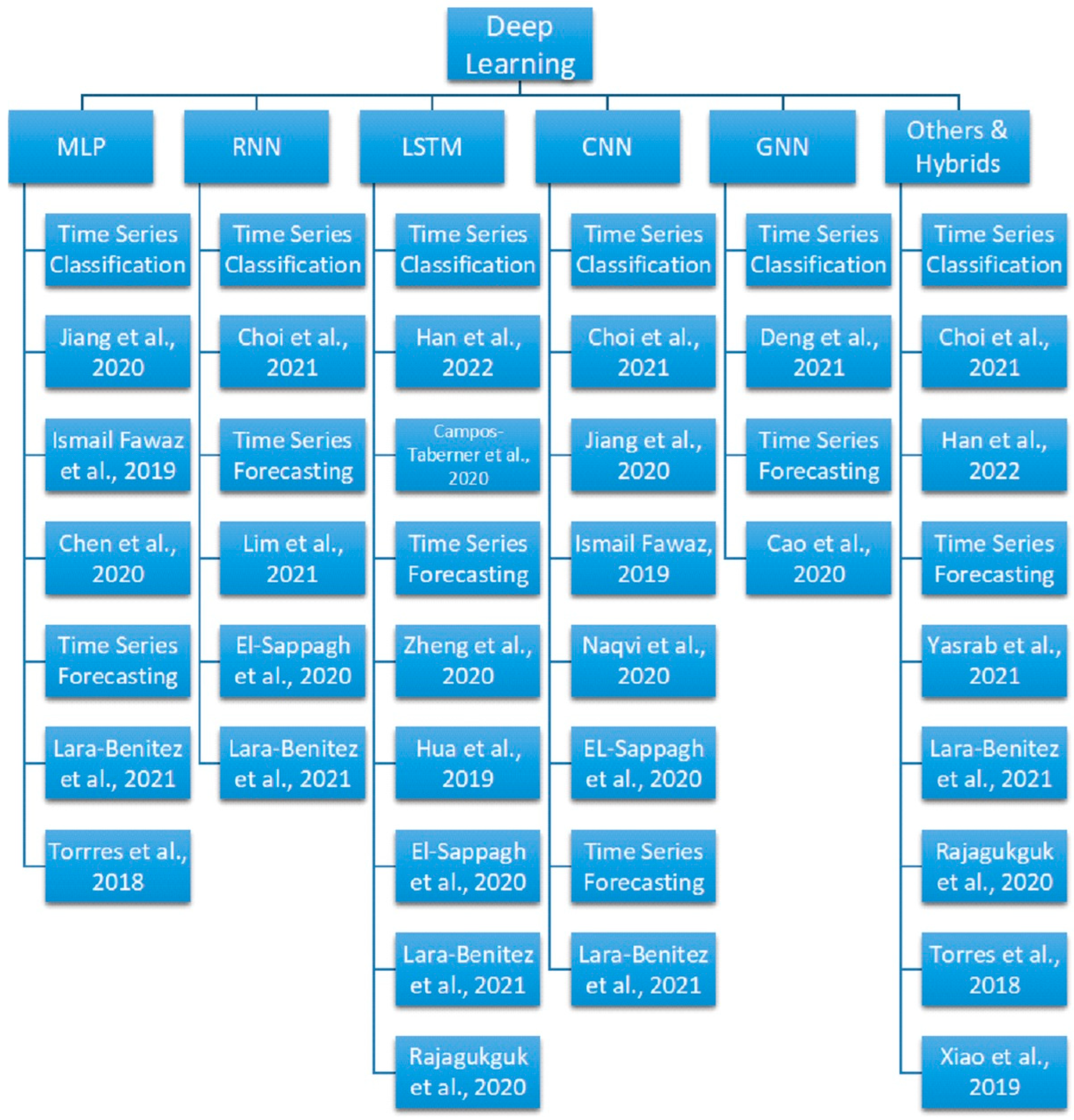
2. Advances in Deep Learning Methods for Time Series Modeling

Deep Learning is capable of modeling the complex non-linear relationships among the variables, while traditional neural network needs to assume that all input vectors are independent, which may lead to its ineffectiveness for sequential data prediction [30]. Comparing DL with the conventional time series methods [13,31], it is found that Deep Learning models can give better representation and classification. Cai et al. [31](2019) investigated the day-ahead multi-step load prediction of commercial buildings with RNN and CNN against autoregressive integrated moving average with exogenous inputs (ARIMAX), a popular traditional time series method for the time series modeling of load forecasting. The results show that the CNN approach with a direct multi-step procedure can perform better than the seasonal ARIMAX by a 22.6% improvement in prediction accuracy. This illustrated that the Deep Learning hierarchical structure may have the capability to handle data-dependent uncertainty better. It is also shown that the long-term trends can be explored better when the preprocessing tool of the moving averages method is deployed for smoothing the short-term fluctuations. Mahmoud and Mohammed [13] presented a survey of Deep Learning models, such as CNN, RNN, LSTM, GRU, deep autoencoders (AEs), restricted Boltzmann machines (RBM), deep belief networks (DBNs), in the time series forecasting of electricity load and price, solar power, and finance, with comparison results showing that DL performs better than classical methods.
After discussing the advantages of deploying DL methods with time series data, the following Table 1 shows a synthetic summary of the advances in Deep Learning techniques for real-world sensor time series applications, followed by a detailed description of the corresponding methods, motivations, and advantages. The following Figure 1 shows the tree diagram grouping the popular Deep Learning methods for sensor time series classification and forecasting tasks covered in this survey.
Multi-layer perceptron (MLP), recurrent neural network (RNN), Long Short-Term Memory network (LSTM), convolutional neural network (CNN), graph neural networks (GNN), deep belief network (DBN), autoencoder (AE), and neural networks with an attention mechanism are popular DL methods that have been used by the authors in this survey.

2.1. Multi-Layer Perceptron

MLP is the most conventional and simplest Deep Learning structure and is fully connected (FC) between layers. All the neurons in one layer are connected to every neuron in the nearby next layer. This means that each time series record is assigned its own weight, and the temporal information is not utilized [35]. During the training phase of the MLP, the weight between the neurons of two nearby layers can be estimated by the minimization of cost function through gradient descent optimization. The computing of the gradient of the cost function is used in the back-propagation algorithm.
Jiang [34] conducted a comprehensive evaluation of the Deep Learning methods (MLP, CNN, and ResNet) against a conventional machine learning method—the nearest neighbor. The 1-NN classifiers are deployed with eight different distance measures. A total of 128 univariate time series datasets about image, motion, and sensor from the UCR Time Series Classification Archive [49] were tested for the classification performance of the models. The experimental results showed that the Deep Learning methods could have better performance than the nearest neighbor, but their difference is not significant when appropriate distance measures are deployed for the nearest neighbor based on the types of the time series datasets.
Ismail Fawaz et al. [35] comprehensively evaluated the performance of three popular structures of Deep Learning for time series classification (TSC), i.e., MLP, CNN, and Echo State Network (ESN). The Deep Learning models for TSC tasks can be classified as generative and discriminative approaches. The essential structure of ESN is the reservoir, a sparsely connected random RNN with random initialization in the hidden layers. Jaeger and Haas [50] invented the ESN in 2004 for time series forecasting for wireless communication tasks. The evaluation was conducted with the 85 univariate time series datasets of the UCR/UEA archive [51] and 13 MTS datasets from Baydogan’s archive [52]. For univariate time series applications, a one-dimensional CNN model is used, and the filter can be viewed as performing a non-linear transformation for the time series. For multivariate time series, the dimensions of the filter are set to be the number of dimensions of the time series. For time series classification, the final layer is the discriminative layer which can assign probability distribution for the class variables of the time series concerned. The results supported that end-to-end Deep Learning is able to reach state-of-the-art performance for TSC tasks.
Chen et al. [41] presented a Deep Learning method based on MLP for equipment reliability prediction with sensor time series data. Condition monitoring for equipment and its maintenance prediction is important for smart manufacturing. It is desirable to conduct maintenance before the machine failure happens. The experiment was conducted with a reliability test of a cylinder in the small trolley of vehicle assembly plant. As it takes longer to complete each operation for an aging cylinder, the cylinder operation duration can serve as the time series inputs for the Deep Learning method. The results show that the Deep Learning method can perform much better than conventional machine learning methods.
Lara-Benitez et al. [45] compared the performance of seven popular Deep Learning algorithms against twelve time series forecasting tasks. Time series forecasting is the process of utilizing relevant historical time records to determine future values. When deploying CNN for time series modeling, causal convolutional filters are used to ensure that forecasting is made only based on past information in the time series [53]. The same as standard CNN, temporal CNN also shares the same assumption that the relationships among the time series variables are time-invariant. In attention mechanisms, the temporal features of the time series signals can be aggregated with the dynamical generation of weights by the attention layers. The attention network can pay more attention to the significant historical event, no matter how far back it is in the key-value lookup window. The Deep Learning models are MLP, four models of recurrent networks (Elman RNN, LSTM, Echo State Network, GRU), and two convolutional networks (CNN and Temporal Convolutional Network). The twelve public datasets cover time series applications like finance, industry, solar energy, tourism, traffic, and internet traffic. The evaluation results showed that LSTM performs the best, while CNN can also make accurate and stable forecasting with less computational requirements. Another performance comparison of Deep Learning methods can be found in Torres et al. [54], making a summary of the satisfactory time series forecasting applications of the popular Deep Learning models (ENN, LSTM, GRU, BRNN, MLP, CNN, and TCN) in the sectors like energy, environment, finance, health, industry, and image. The practical tip on how to set hyper-parameters has also been covered. The four main types of hyper-parameter optimization methods are trial-error, grid, random and probabilistic.
Torres et al. [47] proposed a Deep Learning approach that was based on the H20 package written in R with the grid search method for hyper-parameter optimization and implemented in the Apache Spark cluster environment. As the manufacturing cost for solar panels decreases, solar energy is becoming much more popular. It is predicted that 30% of the total electricity sources will be from solar energy in Australia by the year 2050 [55]. Factors like cloud cover, rainfall, solar radiation, and temperature can affect the generation of solar energy significantly and make the forecasting of solar energy generation difficult. The dataset is the two-year time series of PV power with 30 min observation interval. Its performance was compared with pattern-sequence-based forecasting (PSF) and conventional neural networks. The experimental results supported that the Deep Learning approach is very suitable for the solar energy forecasting task.

2.2. Recurrent Neural Network

RNN is designed with a state for the information at time steps such that it can handle sequence data element-wise [56]. As it can maintain the dependencies among the time series elements, RNN has gained success in different fields such as image captioning, machine learning translation, speech recognition [57], and weather forecasting [58]. Elman Neural Network (ENN) is an RNN model with a new hidden layer called the context layer, which makes it capable of data sequence prediction. Nevertheless, RNN faces difficulties due to the vanishing and exploding gradient problems during its training process. This disadvantage of the vanishing gradient problem can be amplified when considering long-range dependent relationships.
Choi et al. [32] focused on the frontier time series anomaly detection methods and described how the methods model the interrelationship among variables and how the temporal context was learned. Time series anomaly detection is about the identification of unexpected events from the time series data. Because of their learning capability for large-scale sequences, Deep Learning methods contribute significantly to multivariate time series anomaly detection. Nevertheless, most of these methods have been developed for very specific applications, and sufficient domain knowledge is necessary [32]. Benchmark datasets of the water treatment test-bed, the water distribution pipelines, and the Mars Science Laboratory rover were used to compare the performance of the methods (RNN, CNN, hybrid, and attention). The result highlights that there is no single Deep Learning method that can fit universally with all the time series tasks. Even though emerging Deep Learning methods show encouraging results for multivariate time series anomaly detection, most of these methods cannot explain the relationships among the sensors and thus have limited ability to explain the deviations of the anomalous events.
Lim and Zohren [42] summarized the recent trends of Deep Learning models and hybrid models. Hybrid methods combining quantitative time series models with Deep Learning may address these limitations and improve the overall forecasting performance [42]. A hybrid model may be able to incorporate domain experts to feed the Deep Learning model with prior information while addressing the issues associated with small datasets and overfitting. Exponential smoothing RNN (ES-RNN) serves as a good example of how the exponential smoothing module can help the RNN by addressing the non-stationary trends of the time series by winning the M4 competition [59].
El-Sappagh et al. [44] presented an ensemble Deep Learning approach of stacked CNN and Bidirectional LSTM (Bi-LSTM) models for AD progression detection. The temporal information from sensor monitoring of chronic disease can be helpful for progression detection, while the progression of chronic Alzheimer’s disease (AD) may be delayed if it can be predicted at an early stage. The data of AD patients are heterogeneous multimodalities. Bi-LSTM is a special type of LSTM that can explore the dependencies of both previous and future states [6]. For time series prediction with Bidirectional LSTM, once a forecast is available in training, this value can be utilized for the subsequent readjustment process. This may result in a deeper understanding of the context concerned. The model can handle the fusion of the five different types of time series data along with background knowledge. The stacked CNN and Bi-LSTM models are capable of extracting both local and longitudinal features of the modality, and the system can make predictions based on these resultant features. The time series data from the Alzheimer’s Disease Neuroimaging Initiative were used, and the results support the superior performance of the proposed ensemble Deep Learning approach. For traditional methods to succeed in structural health monitoring, suitable preprocessing of the raw sensor time series data is nearly always needed. Dang et al. [60] applied four popular Deep Learning models, i.e., MLP, LSTM, 1D CNN, and CNN, for structural damage detection with raw time series data. No feature engineering procedure like extracting structural characteristics was performed. Three different structures covering small to large structures were tested. The experimental results support that 2D CNN is the most reliable, even though the computational time of 2D CNN is also the highest among the models.

2.3. Long Short-Term Memory

Hochreiter and Schmidhuber [61] designed a new RNN model, called Long Short-Term Memory (LSTM), with an internal memory unit and gate mechanism, for addressing the issues of vanishing and exploding gradient during RNN training. A self-feeding loop is used in the inner layers of LSTM that can learn time-based correlations such that knowledge from previous inputs can be used in the analysis of the present inputs. The three gates implementation [6] of LSTM can reduce the effects of the vanishing gradient problem faced by RNN. The three gates are the forget gate, update gate, and output gate. The forget gate is to determine what information should be kept or not. The update gate is to determine what new information should be utilized for updating the memory state. The output gate is to determine the output value that will serve as the input in the next hidden unit. This design can enable the keeping of longstanding related information while forgetting unrelated information. Thus, LSTM has the capability to process the long-term dependencies of information in temporal datasets and is deployed for applications like speech recognition, traffic prediction, and weather forecasting. The Gated Recurrent Unit (GRU) is designed with a less complex RNN structure than LSTM [62] but can also remember useful information and explore the long-term dependencies of the variables. A GRU has only two gates, i.e., the update gate and the relevance gate. The update gate is to determine if the memory state is to update or not. The relevance gate is to determine how related the previous memory state is for computing the next candidate. As GRU has only two gates, it requires fewer parameters and computational time than LSTM [63] while still keeping the capability for handling very long-range relationships among the time series.
Han and Sanchez-Azofeifa [36] investigated the leaf and wood terrestrial laser scanning (TLS) time series classification with Fully Convolutional Neural Network (FCN), LSTM-FCN, and Residual Network (ResNet). CNN has been found to be capable of performing time series classification satisfactorily, as its multiple filters can produce multiple discrimination features for classification from the temporal inputs [35]. It is also found that the combined LSTM-FCN method can further improve the time series classification results by FCN [64]. TLS point cloud data are useful for classifying the leaf and woody components, and thus the leaf area index and wood area index. The TLS time series point clouds were observed from seven broad-leaved trees (Ulmus americana). The experimental results showed that all three models work better with multivariable time series than with univariable time series. The three models can also work better than previous methods, and all these three models produce similar performances on the testing time series.
Campos-Taberner et al. [37] investigated the interpretability of a 2-layer Bi-LSTM network for the classification of land use in Valencia, Spain, with Sentinel-2 time series data. Added-noise permutation procedure was employed in both temporal and spectral domains for evaluating the impact of different spectral and temporal features on the accuracy rate. The experimental results showed that the overall accuracy of 98.7% achieved by the proposed method is better than other classification approaches. The proposed system can also show the relevance of predictors and highlight that the red and near-infrared Sentinel-2 bands contain the most helpful information, while the summer time series data is most useful among the temporal information.
Zheng and Huang [39] deployed the Deep Learning LSTM network for the forecasting of traffic flow time series. In an intelligent traffic system, the accurate forecasting of traffic flow may help to reduce urban congestion. The traffic flow time series from OpenITS with 5 min intervals in ten days was used, and its performance was evaluated with the traditional statistical method (ARIMA) and the conventional machine learning method (BPNN). The results support the superior prediction accuracy of the LSTM model, with the mean absolute percentage errors of ARIMA, BPNN, and LSTM at 20.97%, 9.06%, and 4.82%, respectively.
Hua et al. [40] deployed the Random Connectivity LSTM (RCLSTM) for traffic prediction and user mobility of telecommunication problems in order to reduce the computational requirement of LSTM. In RCLSTM, the neurons are connected stochastically, and some sparsity can be achieved in this random sparse graph model to reduce computing time. RCLSTM is found to be suitable for latency-stringent tasks like traffic time series. Another similar task is the evaluation of the traffic time series data from the GEANT backbone network by Uhlig et al. [65]. The experimental results showed that the forecasting performance of RCLSTM is similar to the traditional LSTM while successfully reducing the computational time.
Rajagukguk et al. [30] investigated the prediction performance of solar irradiance and photovoltaic (PV) power with four Deep Learning models against conventional machine learning methods. As solar energy is renewable, solar photovoltaics has gained popularity in the generation of electricity. For the PV prediction, the popular input time series data are the temperature, humidity, and wind speed. The experimental results confirmed that all four Deep Learning models, i.e., RNN, LSTM, GRU, and CNN-LSTM, can perform the prediction better, with CNN-LSTM achieving the best performance but also needing the longest training time period. In the hybrid model CNN-LSTM, the CNN layers can perform the feature extraction of the input time series, while LSTM for sequence prediction. CNN-LSTM has been designed with the capability to handle temporal prediction tasks and applied in many real-world applications. Experimental results like [66] also supported the consistently better performance by CNN-LSTM over LSTM for precipitation prediction.

2.4. Convolutional Neural Network

CNN is another popular neural network for time series modeling. CNN is a DL method of interconnected feedforward network architectures consisting of a sequence of convolution, pooling, activation layers, and, finally, fully connected layers [67]. Filtering operation is performed in the convolutional layers through a feature map. Local confluences of features are identified from the preceding layer through discrete convolution. Thus, this type of model becomes known as a convolutional neural network. The pooling layer is for reducing the input size and avoiding overfitting. The input for the last dense layer is the flattened features from the convolutional and pooling layers, and the forecasting is made in this dense layer. 1D CNN can be deployed for simple applications, while more sophisticated models, like CNN-Net, Enoded-Net, and CNN-LSTM, have more advanced structures like larger kernel size and denser layers.
Naqvi et al. [38] deployed a CNN model for detecting changes in gaze from the face and left- and right-eye images. Driver time series data is helpful for the real-time classification of normal and abnormal driving and, thus, for reducing aggressive driving. The near-infrared (NIR) camera sensor is employed here to construct a large database of driver facial emotion and gaze. The Dlib facial feature trackers were employed to identify the region of interest (ROI) before feeding to the CNN model. The experimental results supported the outstanding performance of the CNN model.

2.5. Graph Neural Network

GNN is a neural network that processes the data with representation in graph domains, like in chemical compounds, images, and web [68]. Graphs can be classified as cyclic, directed, undirected, or a combination of these three. GNNs have been found useful for applications including chemistry, citation networks, environmental condition forecasting, molecular biology, physics, and social networks. A few DNN topologies may indeed be viewed as GNN, for example, with CNN considered as a GNN with graphs of pixel-per-grid grids.
Deng and Hooi [33] developed a Graph Deviation Network (GDN) model for discovering the relationship graph among the sensors and for detecting deviation from normal patterns. Graph neural networks can model the complex patterns in data of graph structure, with the node state influenced by its neighbor note states. Velickovic et al. [69] developed the graph attention network (GAT), which employed the attention function for evaluating the various weights for various neighbors during aggregation. A difficulty for a typical GNN model is that the graph structure is needed as an input, while this structure may not be known in advance. The proposed system consists of sensor embedding, graph-structured learning, graph-attention-based forecasting, and graph deviation scoring. The system is tested with two large-scale sensor time series datasets of water treatment systems (SWaT and WADI). The experimental results supported the performance of the proposed system, while the interpretable output can assist users in better understanding and localizing anomalies.
Cao et al. [46] presented Spectral Temporal Graph Neural Network (StemGNN) with Graph Fourier Transform (GFT) for capturing inter-series correlations and Discrete Fourier Transform (DFT) for temporal correlations. A difficulty for multivariate time series is the complexity involving both the temporal correlations of intra-series and the correlations of inter-series simultaneously. The spectral representations obtained with GFT and DFT enable the Deep Learning modules to have clear enough patterns for the analysis. The experimental results from ten real-world time series public datasets (from energy, electrocardiogram, and traffic sectors) confirm the performance of the proposed StemGNN.

2.6. Others and Hybrids

Hinton and Osindero et al. [70] developed the first model and training algorithm for a deep belief network (DBN) in 2006. DBN has a hierarchical structure with a large number of stacked restricted Boltzmann machines (RBMs) and utilizes a greedy layer-by-layer learning approach with fine-tuning. The RBMs can efficiently extract the features for the initialization of feedforward neural networks, hence improving the network generalization capability. In each RBM, there is both a visible layer and a concealed layer consisting of neurons. While the RBM’s layers are interconnected with each other, the units among each layer are not. The updating of the network parameters can be done with a SoftMax classifier.
Autoencoder utilizes a feature learning paradigm that can learn para-metric maps directly from inputs to corresponding representation [71,72]. An AE consists of an encoder and a decoder. The encoder is for feature extraction, while the decoder is for mapping the feature space back to the input space. The structure of the encoder and decoder is an input layer, hidden layers, and an output layer. Back-propagation algorithm is deployed for updating the weights of the hidden layers. Deep AE can serve as a data-driven approach for learning feature extraction automatically.
Neural networks with an attention mechanism have succeeded in time series applications [73]. These networks can dynamically control the mapping from the inputs to the outputs intelligently with other knowledge of the task. The transformer model is based on an encoder–decoder architecture of these networks. The input is fed to the encoder, which consists of a stack of encoders. Then, the transformer can generate the output based on the encoded input and previous outputs in the decoder as well. A clear advantage of transformers is the access to any points in the past, no matter how far their distances are, leading to the capability to discover the long-term dependencies among the time series data.
Yasrab et al. [43] designed a Generative Adversarial Network (GAN) for forecasting the expected growth of the plant. Plant phenotyping is the investigation of plant trait growth and other quantitative parameters and may be automated with the help of Deep Learning. GAN is usually developed from CNN and is formed with two networks, i.e., the generator and the discriminator. Both networks can learn together by competing with each other to generate new examples of synthetic data. Segmentation masks of shoot and root were generated to predict the plant system in the future. Two public datasets (Arabidopsis and Brassica rapa plants) were used. The evaluation results illustrated that the proposed system can reach the level with annotation by an expert.
Xiao et al. [48] developed a Convolutional Long Short-Term Memory (ConvLSTM) model to utilize the spatiotemporal correlations of sea surface temperature (SST) for its short and mid-term prediction. In the global ocean, SST has a significant influence on the marine ecosystem. SST time series data from 36-year observations by satellite was used to evaluate the ConvLSTM against the persistence model, support vector regression model, and LSTM models. When handling spatiotemporal data by fully connected LSTM (FC-LSTM), it is noted that the spatial correlations can be lost [66]. To address this issue, the ConvLSTM replaces the FC-LSTM matric multiplication with convolution operation in the transitions. This is to ensure that the model can explore both spatial and temporal correlations. The experimental results confirmed that ConvLSTM performs better than other methods for the one-to-ten-day-ahead prediction of SST time series.

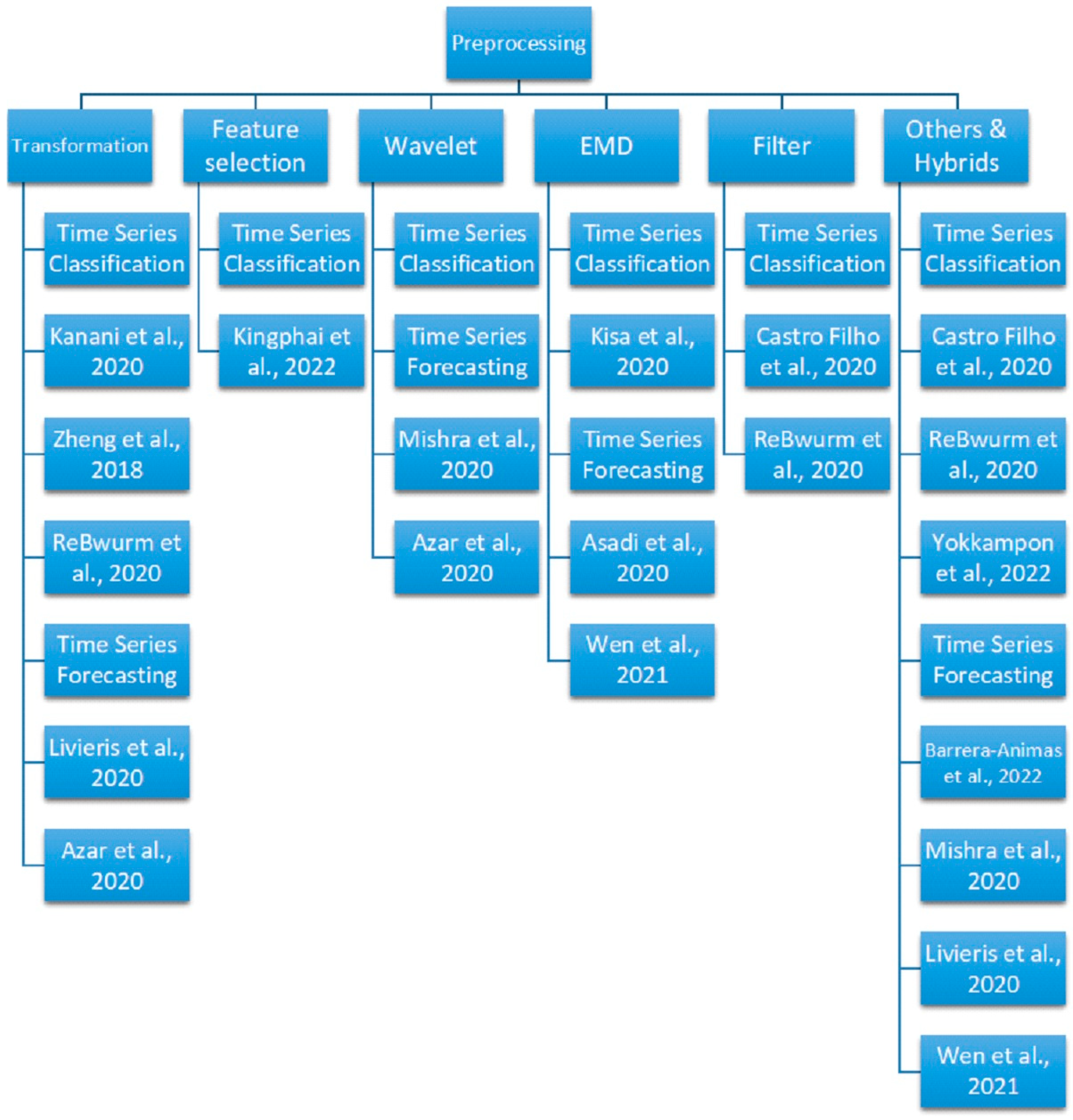
2.7. Advanced Preprocessing and Deep Learning Applications

Feature engineering can be very important in the data preprocessing stage before feeding data to the Deep Learning models by significantly reducing the computational requirements for unnecessary features. Its importance is highlighted in the work of Elsayed and Thyssens et al. [74], which evaluated the time series forecasting performance of eight Deep Learning methods against the traditional machine learning method—the Gradient Boosting Regression Tree (GBRT). External features were utilized for the target values, and data flattening can obtain the one input instance for GBRT. The evaluation was conducted with nine datasets covering air quality, electricity, finance, solar energy, and traffic. The results showed that the window-based transformation could enable GBRT to achieve the best forecasting performance over the Deep Learning models, covering various types like matrix factorization, RNNs, LSTMs, and bi-directional LSTM models. It is shown that simpler machine learning models with efficient feature engineering can outperform the frontier Deep Learning methods without feature engineering. Dablander and Bury [9] highlighted the importance of preprocessing by showing that the DL model cannot extract enough relevant features for classifying the stationary AR(1) processes without detrending or with a Gaussian filter. The results showed that the method might learn unique features related to a Lowess filter instead of the relevant features of the system near the bifurcation. Thus, careful planning is needed when deploying the preprocessing models.
The following Table 2 highlights the most recent case studies that advanced preprocessing is still needed, along with the Deep Learning methods, for modeling different popular types of sensor time series. In Table 2, a synthetic summary of the application fields, the advanced preprocessing techniques, the DL methods, accuracy, and brief application details is presented, followed by a more detailed description of the corresponding methods, motivations, and advantages. The following Figure 2 shows the tree diagram for grouping the popular preprocessing methods for sensor time series classification and forecasting tasks covered in this survey.
Kanani and Padole [75] presented a preprocessing framework that can increase the electrocardiogram (ECG) classification accuracy of the Deep Learning methods significantly, with a higher than 99% accuracy rate. ECG time series signals are very efficient for the monitoring of cardiovascular health, with abnormal heartbeats detected from the ECG patterns. The labeled MIT-BIH Arrhythmia dataset, which has ECG time series signals of five different classes, was tested. The proposed preprocessing steps include the squeezing and stretching of the signal along the time axis and the amplifying and shrinking of the amplitude of the signal. It is shown that these transformations do not change the characteristics of the signals and can be regarded as completely lossless transformations here.
Kisa et al. [76] deployed an adaptive preprocessing method with empirical mode decomposition (EMD) was proposed to handle this nonstationary time series, as the surface electromyography (sEMG) time series is nonstationary and nonlinear. sEMG can be employed to measure the electrical activity of human muscles. The recognition of human movements is useful for applications like human–computer interaction (HCI). The sEMG hand gesture time series data was obtained with a sensor device of surface bipolar electrodes with 30 healthy volunteers. EMD can serve as a non-linear filter to decompose the input time series into several intrinsic mode functions (IMFs). The outputs of the IMFs were then fed into the Deep Learning model CNN based on Residual Networks (ResNet) for gesture classification. It is found that the IMFs can improve the validation accuracy of the original time series from 94.22% to a maximum of 99.73%.
Zheng et al. [8] investigated the segmentation and transformation methods for their effectiveness in data preprocessing for Deep Learning algorithms. In HAR tasks, segmentation methods are essential as raw inertial time series can have very large fluctuations. Five segmentation options of five different segment lengths were evaluated with four transformation methods, i.e., raw plot, multichannel, spectrogram, and spectrogram with shallow features. The experiment was conducted with datasets of eight daily activities from wearable sensors, car workshop maintenance activity data, etc. The results showed that the classification accuracy increases along with an increase in segment length, and the multichannel method can perform the best for the HAR tasks. The overall accuracy is 97.2%, which is better than many other machine learning models.
Castro Filho et al. [77] applied a two-stage noise scheme for preprocessing SAR time series, as there are inevitable noises like speckles for Synthetic Aperture Radar (SAR) images. SAR sensors can be employed for mapping the rice-growing regions and constructing continuous time series data. The SAR data is very useful for monitoring short phenological stages and raising the classification capacity. 3D-Gamma filter was used to eliminate the speckle, and the method of Savitzky and Golay [84] was employed to smooth the time series. The processed time series was fed to two Deep Learning methods, the Long Short-Term Memory model and the Bidirectional LSTM model, for mapping rice crops with SAR sensor time series from West Rio Grande do Sul (Brazil). The results were compared with conventional machine learning models, with BiLSTM showing the best performance in the McNemar test.
ReBwurm and Korner [78] investigated the effectiveness of Deep Learning models for the classification of crop type based on raw and preprocessed Sentinel 2 satellite time series data. With the advance of remote sensing technologies, the amount of the Earth observation time series data has been greatly increasing over recent years. While many traditional models for remote sensing applications require preprocessing and feature extraction, ReBwurm and Korner [78] checked if the current Deep Learning methods are able to utilize the raw time series data directly without data preprocessing. Atmospheric correction, filtering of cloud temporal observations, focusing on vegetative periods, and masking of clouds, which are typical preprocessing methods for satellite time series, have been applied. Additionally, 1D-convolutions, recurrent neural networks (RNN), and the self-attention model of the encoder architecture of the Transformer network [85] are deployed and evaluated. The results show that self-attention and RNN can perform better for raw data, while the preprocessing process can improve the results for all three methods satisfactorily.
Kingphai and Moshfeghi [79] employed seven Deep Learning models, i.e., convolutional neural network (CNN), Stacked Gated Recurrent Unit (SGRU), Bidirectional GRU (BGRU), BGRU-GRU, LSTM), Bidirectional LSTM (BiLSTM), and BiLSTM-LSTM, for classifying mental workload (MWL) levels from electroencephalography (EEG) time series signals. MWL can lead to a better understanding of human performance in complex environments. EEG time series can be utilized for classifying the mental workload level of a human subject. The dataset STEW contains signals from 48 subjects in the resting and working states. Preprocessing is needed because there is usually noise in the EEG signals. The independent component analysis based on ADJUST (ICA-ADJUST) by Mognon et al. [86] was found to be the most effective preprocessing tool for this dataset by Kingphai and Moshfeghi [87]. Kingphai and Moshfeghi [79] extracted four groups of features (frequency domain, time domain, linear domain, and non-linear domain) for the Deep Learning models. The results showed that BiLSTM-LSTM performed best with 94.75% accuracy for classifying resting vs. working states, while BGRU-GRU was best for classifying low vs. moderate vs. high MWL levels with 83.03% accuracy.
Yokkampon et al. [80] deployed multi-scale attribute matrices as the preprocessing tool for transforming the multivariate time series to develop a multi-scale convolutional variational autoencoder for unsupervised anomaly detection of multivariate sensor time series datasets. The attribute matrices can utilize the pair-wise inner product of the time series among segments and effectively characterize system states of the time series. The identification of anomalies is about detecting data points that deviate significantly from their expected values. There are three types of time series anomalies: (1) point anomalies, which refer to outlier points; (2) contextual anomalies, which differ significantly from typical points of the same context; and (3) collective anomalies, which refer to the existence of a subset of time series data points with a significant difference from the other points in the whole dataset [88]. Anomaly detection can be employed in many real-world cases, like fraudulent transaction detection, sensor network fault analysis, and abnormal equipment monitoring. The proposed model was tested with four publicly available benchmark datasets: the time series data by the Australian Centre for Remote Sensing, the Wafer time series dataset of semiconductor microelectronics fabrication, the Emotiv EEG Neuroheadset time series dataset, and Opt handwriting dataset. The experimental results show that the model performed better than other baseline methods.
In the investigation by Barrera-Animas et al. [58], before feeding the time series data into the DL models, the feature selection process was achieved with the correlation matrix (CM), which is computed with the Pearson correlation coefficient for the 43-dimensional datasets. Rainfall prediction is complicated because of its nonlinear characters. Spatial information like latitude and longitude and atmospheric information like humidity, pressure, temperature, and wind speed may be utilized for the forecasting models. Barrera-Animas et al. investigated the effectiveness of Deep Learning models, including LSTM, Stacked-LSTM, and Bidirectional LSTM, with the conventional machine learning (ML) model XGBoost, and also automated machine learning (AutoML) with the TPOT tool [89], which can be regarded here as an ensemble of ML models. OpenWeather data of five UK cities from 2000 to 2020 were evaluated. Highly correlated features will be eliminated. The experimental results highlighted that the Stacked-LSTM with two hidden layers and the Bidirectional LSTM could obtain the best performance in rainfall forecasting.
Mishra et al. [81](2020) evaluated the wind predictions with five Deep Learning methods against three data preprocessing tools. The five methods are the attention mechanism (Attention) of sequence-to-sequence encoder–decoder architecture [90], deep convolutional network (DCN), deep feed Forward (DFF), recurrent neural network (RNN), and LSTM. The dataset is the time series of the temperature and wind power variable. Discrete wavelet transformation and fast Fourier transformation (FFT) are employed to transform the time series dataset before feeding to the Deep Learning models, while inverse transformation was applied to the DL model outputs before making predictions. The experimental results showed that Attention and DCN work the best with wavelet and FFT, while some other models work better with no need for data preprocessing.
Livieris et al. [10] proposed a preprocessing framework to further improve the efficiency and reliability of the Deep Learning methods. Iterative transformations and augmented Dickey–Fuller test were applied to the time series data for obtaining stationary processed time series data before feeding to the Deep Learning model. The Ljung–Box Q test was employed to check the autocorrelation of the model’s errors. Time series data from energy section, stock market, and cryptocurrency were tested, and the experimental results showed that the proposed preprocessing framework could enhance the efficiency, accuracy, and reliability of the Deep Learning LSTM and CNN-LSTM models considerably. Livieris et al. [91] continued their work on the investigation of the preprocessing framework for Deep Learning models. On top of their previous focus on the transformation of non-stationary time series to stationary by differencing the time series, the raw time series is now subject firstly subject to the exponential smoothing method, which can transform the raw data to a de-noised version. This process is to increase the quality of the time series data and thus improve the prediction capability of the Deep Learning model CNN-LSTM. The experimental results with cryptocurrency, energy, and stock markets confirmed that the preprocessing framework could significantly achieve its objective of further improvement for the Deep Learning models.
Asadi and Regan [1] employed the time series decomposition method to obtain the short-term, long-term, and spatial patterns in the proposed preprocessing framework. The short-term patterns of the spatial time series were explored with the fuzzy clustering method, which can group neighboring time series together according to the checks on the residuals of the time series. These residuals in spatial time series can provide meaningful patterns with neighboring locations, like showing how the traffic is evolving in the road network. The traffic flow time series dataset was tested, and the method can obtain better results than both the baseline and state-of-the-art methods.
Wen et al. [82] presented a survey of the data augmentation methods that are specifically designed for handling time series datasets. Because many real-world applications like medical time series or anomaly detection time series face the problem of not having enough labeled data, it can be very helpful to have an effective way that can enlarge the size and improve the quality of the training data during deploying Deep Learning on time series datasets. Data augmentation has been found very suitable for this task, as it can generate data synthetically for unexplored input space with correct labels. Not only basic data augmentation methods, like time domain and frequency domain, but also advanced methods, like decomposition-based methods, statistical generative models, and deep generative models, are covered in the survey by Wen et al. These augmentation methods are found to be effective in time series classification, time series anomaly detection, and time series forecasting.
Azar et al. [83] developed a compression module for both univariate and multivariate time series data with the discrete wavelet transform and the error-bound compressor Squeeze (SZ). On-board processing and compression algorithms can reduce the problems associated with the transmission of large data volumes in applications of the Internet of Things (IoT). This preprocessing procedure is especially important for the sensor systems in IoT, as they may only have very limited bandwidth, memory, and computational power. The processed time series data is then sent to the Deep Learning models (Resnet, LSTM-FCN, GRU-FCN, FCN) for time series classification. The Fully Convolutional Network (FCN) deployed here consists of a convolutional layer with filters, a batch normalization layer, and then a ReLU activation layer. The experiment was conducted with time series datasets (UCR, UCI, and UEA) from sensors of ECG, motion, etc. The results supported that the compression approach can achieve a high compression ratio, while its time series denoising capability enables the Deep Learning module to achieve satisfactory classification accuracy.

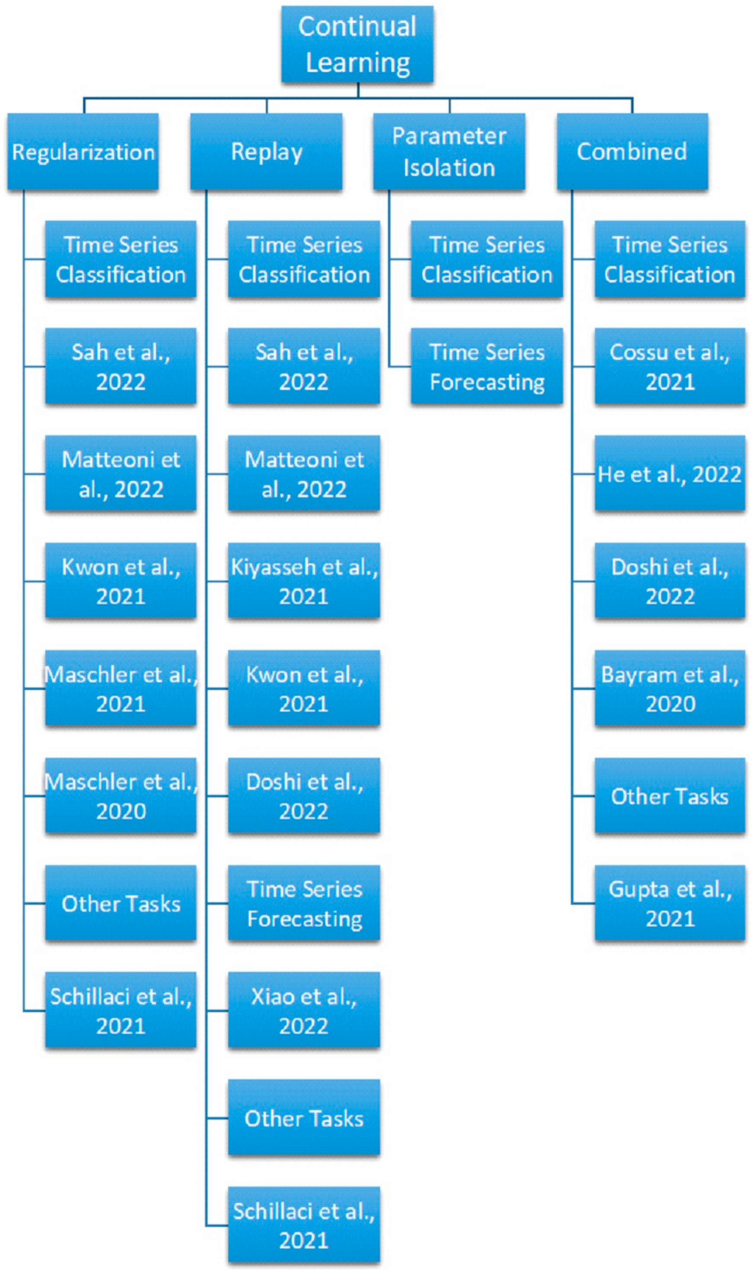
3. Advances in Continual Learning Methods for Time Series Modeling

In the previous section, applications of Deep Learning models and preprocessing methods in different real-world time series scenarios have been reviewed. Limitations of Deep Learning models include a strict static requirement for the underlying process [92]. Post-deployment changes are not uncommon in the real world, but the DL methods are usually of fixed network structure after being deployed. When DL models are fed with data not following the independent and identically distributed (i.i.d.) assumption, destructive interference may occur and cause performance degradation [93]. Continual learning may be deployed to address these difficulties faced by DL models in such a way that Deep Learning models may benefit from continual learning to become capable of learning continually with adaptability.
A major characteristic of continual learning is its sequential learning process. At each time, only a small amount of the input data is available. Other names for CL include lifelong learning, sequential learning, and incremental learning. Mathematically, the continual learning for both classification and time series regression problems can be expressed as follows [94]: Let Τ = ( Τ 1 , , Τ m ) represent the m tasks that arrive in sequence. For task Τ i i = 1 , 2 , , m , there exist N instances of labeled time series data D i = x i , r , y i , r r   =   1 N . Here, time series x i , r Χ i is associated with the corresponding target y i , r Υ i . For classification tasks, the target space Υ i refers to class labels. For time series regression tasks, the target space Υ i refers to real numbers. A constraint of continual learning is that for any task Τ i , there exists no access to the data of previous tasks Τ j j = 1 , , i 1 . The common goal of each task is to learn a solver model M i , such that M i : Χ i Υ i , with trainable parameters θ i and estimated target y ^ i , r = M i x i , r ; θ i . Let L y i , r , y ^ i , r ; θ i represent the training objectives. For classification problems, this can be the standard cross-entropy loss, while for time series regression problems, this can be the squared-error loss. Then,
L i = q N r = 1 N L y i , r , y ^ i , r ; θ i + 1 q i 1 N j = 1 i 1 r = 1 N L y j , r , M i x ^ j , r ; θ i ; θ i
where N refers to the number of instances, and 0 < q 1 refers to the importance assigned to data from Τ i .
There are several popular CL scenarios, like Instance-Incremental Learning (IIL), Domain-Incremental Learning (DIL), Task-Incremental Learning (TIL), Class-Incremental Learning (CIL), Task-Free Continual Learning (TFCL), and Online Continual Learning (OCL). This taxonomy is based on how the incremental batches are divided and which task identifies are available [18]. IIL refers to scenarios where all training samples arrive in batches and belong to the same task. DIL refers to scenarios where task identities are not needed; tasks have different input distributions but the same data label space. TIL refers to scenarios where task identities are available during both training and testing, and tasks have disjoint data label spaces. CIL refers to scenarios where task identities are available only during training and tasks have disjoint data label spaces. TFCL refers to scenarios where no task identity is available and tasks have disjoint data label spaces. OCL refers to scenarios where training samples for each task arrive from the data stream one by one, and tasks have disjoint data label spaces.
Flesch et al. [95] highlighted that for human continual learning, the extensive background statistical knowledge gained from previous unsupervised training might be utilized for rule learning at later stages, though with several conditions, while DNN suffers catastrophic forgetting (CF) problems. CF can be viewed as an issue stemming from the NN stability–plasticity dilemma, and the CF effect is associated with the abrupt loss of previously learned knowledge [17]. Plasticity refers to the NN’s ability to learn new knowledge, while stability means the storing of learned knowledge. CL can be employed in supervised learning, semi-supervised learning, unsupervised learning, and reinforcement learning as well. Shaheen et al. [96] discussed the applications of continual learning for autonomous systems. The real-world systems of vehicles with self-driving capability, unmanned aerial vehicles, and autonomous robotics were highlighted.
Various degrees of constraint simplification for solving the CF issue are imposed in the current methods. There are constraints such as memory, computational power, and data privacy. Nevertheless, there are issues when applying these methods, for example, too rigid constraints that may break the idea of learning continually or too tailor-made for solving a particular type of problem only. Pfulb and Gepperth [97] investigated the CF problems in DNN with a very large number of datasets in visual classification. The large-scale experiments show that no model and dataset is free of the CF problems, whilst a few potential workarounds may enable a few models to become practicable in a few application-level environments. Inspired by open-set recognition, Prabhu et al. [98] presented a model called GDumb, which is not tailor-made for CL tasks. GDumb starts with storing samples greedily in memory as they arrive, and during testing, it proceeds with new model training with samples only in the memory. GDumb is shown to outperform many CL approaches and may serve as an alert to the current progress in CL for classification, with the oversimplifications by some existing CL approaches to the problems resulting in little real-world application value. In the deep autoencoder NN for time series forecasting [99], buffers were deployed with online elastic weight consolidation to learn the probability distribution of the data stream sequentially. A CL model with explicit memory structure was used to address CF in their FFNN model for making long-term financial investment decisions [100]. Chen et al. [101] employed graph neural networks with CL strategies—data replay and parameter smoothing—for transferring learned knowledge to the current model in their traffic flow forecasting framework.
The relationship between neural network architectures and CF was investigated, and it was found that the network width has a significant effect on forgetting. Nevertheless, when increasing the width to address CF, inefficiency problems like long computation time and large energy waste inevitably appear. Lange et al. [17] investigated model capacity, weight decay, dropout regularization, and the stability–plasticity trade-off among continual learners. Lesort et al. [102] investigated the effects of the parameterizations of the DNN output layer on learning and forgetting in CL. The evaluation is conducted in a simplified learning environment, decomposing the model as a classifier part for the output layer and a feature extractor part for the rest of the DNN. Weights modifications, interference, and projection drift can be the causes of CF in the output layer. More knowledge is gained about the continual learning in output layers. Instead of focusing solely on continual learning, Mundt et al. [103] presented a framework combining concepts from CL, open set recognition, and active learning. This holistic approach shows promising results in addressing catastrophic forgetting and robustness for open-world applications.
Current limitations for CL applications include the predominant closed-world assumption when deploying models, which requires that any new data follows the same distribution as those used during training. When this closed-world assumption is no longer valid, the neural networks may give false predictions with unknown situations or with corrupted data [103]. Another limitation is that many current works in CL may not often consider the scalability issue in potential applications, which may have a very large number of sub-tasks and, consequently, huge amounts of samples.
Whilst most of the recent works on CL focus on supervised tasks, the over-specializing of CL training for a single set of environments limits CL generalization to other types of applications [104]. With most recent research focusing on the CL applications for classification tasks, this lack of attention may hinder time series applications like renewable energy forecasting with CL models [99]. Deep Learning methods without the ability to remember old knowledge may not handle well in real-world applications of time series forecasting with non-stationary sequential data [105]. On the other hand, the current CL projects on different time series regression tasks are showing encouraging results. Pham et al. [105] designed a fast and slow learning network for online time series forecasting, with the per-layer adapter for fast learning and associative memory for remembering and recalling repeating past events. CL may be very useful for addressing financial time series problems, which can appear everywhere and are commonly non-stationary [100], and for traffic flow time series forecasting, which is essential for smart transportation. Most current methods of traffic flow forecasting assume static networks [101]. Yet, real-world traffic flow networks change constantly, like possible network modification and the addition of new parts [106].
After the above discussion illustrates the importance of continual learning among the Deep Learning time series applications, a synthetic summary of the advances in continual learning techniques for time series applications is presented in Table 3, followed by a detailed description of the corresponding methods, motivations, accuracy, and brief details. The following Figure 3 shows the tree diagram of the taxonomy of the continual learning methods for sensor time series classification and forecasting.
As it is NP-Hard to find the optimal CL algorithms which can completely avoid catastrophic forgetting [117], polynomial time heuristic algorithms have been proposed to address the CF problems. These CL algorithms can be classified into three families, i.e., regularization-based methods, replay methods, and parameter isolation methods, according to the storage and usage method for task-specific information during the sequential learning process [17]. Combined approaches refer to the mixing of the methods together, and outstanding results can be obtained on benchmark datasets [103]. Another possible taxonomy is of regularization-based approach, replay-based approach, optimization-based approach, representation-based approach, and architecture-based approach [18]. This survey will follow the taxonomy of Lange et al. [17] and Mundt et al. [103].

3.1. Regularization-Based Methods

Regularization-based methods need to utilize an extra regularization term in the loss function for combining previous knowledge during the learning process of new data. Regularization methods focused on how to preserve previous knowledge. Extra loss terms can be deployed to preserve the important weights gained from the learning of former tasks. Elastic weight consolidation (EWC) [118], learning without forgetting (LWF) [119], and knowledge distillation [120] are popular regularization approaches.
Sah et al. [107] investigated the performance of three recent continual learning approaches (A-GEM [121], ER-Ring [122], and MC-SGD [123]) for addressing the catastrophic forgetting in wearable sensors for activity recognition. In a wearable sensor system, it is necessary to have the capability to monitor and recognize activities across users. This sequential learning process is non-stationary and challenging for Deep Learning methods. The PAMAP2 dataset [124] of human activity recognition, consisting of sensor time series data of eight subjects and twelve daily activities, is used for the evaluation. The results showed that MC-SGD performed the best by reducing nearly 29% of the forgetting, while its computational time is still much less than the joint-task training time.
Matteoni et al. [108] developed two benchmarks of human state monitoring of domain-incremental scenarios for CL models. In non-stationary environments, recurrent neural networks for time series data can be of large importance [110], and investigation of the network properties in these situations may lead to a better understanding and applications of CL models. A significant obstacle that hinders the development of CL models is the shortage of enough standard benchmarks of time series datasets for the evaluation of the CL models. The two benchmarks were derived from datasets WESAD [125] and ASCERTAIN [126] of time series classification from physiological sequence data. Different CL models were investigated with these two benchmarks to understand the effects of catastrophic forgetting on recurrent neural networks. Four common CL models, i.e., replay [20], elastic weight consolidation (EWC) [118], learning without forgetting (LwF) [119], and naive and cumulative strategies, were tested. The results showed that all the CL models can mitigate forgetting, but besides the replay model, all other models still can not accumulate knowledge over time.
Kwon et al. [109] comprehensively investigated the performance of three CL approaches—regularization, replay, and replay with examples for deployment in mobile and embedded sensing devices. Most of the existing continual learning methods do not consider the resource requirements and limitations of mobile and embedded sensing devices [127]. Three datasets of human activity recognition, two datasets of gesture recognition, and one dataset of emotion recognition were investigated to find the trade-offs between system performance, storage requirements, computational power requirements, and peak memory requirements among the CL approaches. The results showed that the CL approach of replying with exemplars works best after considering all the trade-offs.
Maschler et al. [113] evaluated the performance of a continual learning approach based on regularization strategies, which mimic the human brain synaptic consolidation, for industrial application. Existing methods for anomaly detection often lack the flexibility to adapt to changes in the manufacturing processes [113], while continual learning can help overcome this issue by providing the automatic capability for adapting formerly learned knowledge to new settings. Real-world metal-forming time series dataset of a discrete manufacturing process was tested, showing promising results for the regularization strategies over the multilayer LSTM approach with no regularization. Online elastic weight consolidation is found to provide better performance than elastic weight consolidation. Maschler et al. [128] evaluated the performance of the regularization strategies against the open-access lithium-ion battery degradation dataset [129] with the LSTM approach for remaining useful lifetime prediction for lithium-ion batteries. The results of these degradation datasets reinforce the findings for the discrete manufacturing process. Network monitoring can produce a huge amount of multivariate time series data that are useful for usage, like network anomaly detection. Gonzalez et al. [130] outlined their conceptual framework of variational autoencoders and dilated convolutional networks for network anomaly detection. The deep generative replay is explored for extending the continual learning capability to the proposed system. The teacher generative model can create synthetic data to imitate previous training examples, while the new student model can learn from current new data and also these synthetic data at the same time. This continual learning module may help to address catastrophic forgetting.
Maschler et al. [114] proposed an LSTM algorithm with elastic weight consolidation for fault prediction in a distributed environment. Continual learning has the potential to serve as a distributed approach for fulfilling the industrial automation need, with Deep Learning performing fault prediction for industrial automation. This is because many real-world restrictions like industrial espionage and legal privacy concern prevent the centralizing of data from factories for the training of the Deep Learning models. NASA turbofan engine dataset [131] was used for performance evaluation. The experimental results showed that their approach could perform effectively with distributed datasets with no requirement for centralized data storage, satisfying the requirements of many real-world manufacturers.
Schillaci et al. [116] developed a continual learning RNN model with episodic memory replay and consolidation driven by prediction errors for transferring the knowledge gained from the greenhouse research facilities to real-world greenhouses. Without the CL capability, this process may otherwise be expensive and risky for the crop due to problems like the requirement of large-scale re-training in the new facility. Sensor time series data may help to better understand the causal models of a dynamic system, and this is very useful for real-world applications. Currently, popular causal discovery methods utilize only static data or pre-processed time series data in advance, making them not very suitable for real-world robotics cases. Continual learning may address this limitation in the causal discovery methods [132] but is under-investigated for robot application [133]. Castri et al. [133] focused on the constraint-based methods for causal discovery and outlined their approach of re-learning the causal model during observed scenario changes and during a new set of interventions. The new inference matric of the causal model is checked against the matric of the old causal model to discover the still valid causal links from the old model for the new model. This approach of only small incremental changes can help the robotic system address the CF problem. CL module can also help the robotic system address the hardware resource limitation. Sensors in a greenhouse can produce time series data like climate time series and leave temperature time series. A better understanding of the complex greenhouse and modeling of these greenhouse time series data can help to predict the effects of intervention better, thus increasing the crop yield. Memory retention is based on congruence against prior knowledge retained in the model, and the experimental results showed that this memory replay strategy could enhance the performance of standard memory consolidation approaches.

3.2. Replay Methods

Replay methods need to store either the raw samples or the generated pseudo-samples from the generative algorithm. These stored previous samples can be replayed to address forgetting during the learning of new tasks. Difficulties for this approach may include the demand for resources of large storage capability and the privacy concerns for storing and deploying samples in real-world applications. Pseudo-rehearsal techniques can handle these difficulties with a generative model instead of storing past samples directly.
Kiyasseh et al. [93] utilized the replay buffer strategy to construct the continual learning model CLOPS from the temporal data in clinics, which is often non-stationary, as multiple clinical sites with various sensors are involved. Acquisition based on uncertainty was deployed for the replay of buffer instances. Four clinical environments involving transitions between data modalities, diseases, clinics, and time are suitable non-stationary scenarios to test the performance of the continual learning approach. The results show that CLOPS performs better in three scenarios than the two other frontier methods—GEM [134] and MIR [135]. He [111] also focused on the target-domain incremental application scenario and data-domain incremental application scenario of continual learning and described how their previous framework, CLeaR, can be extended to learn inputs successively. The framework utilizes the storage of buffered data by a novelty detector. The application of continual learning to the regression scenario for power forecasting was outlined.
Doshi and Yilmaz [112] proposed a new continual learning approach for video anomaly detection. Sensors and cameras in CCTV systems are generating huge amounts of real-time video temporal data, and data size may be too big to be investigated by humans. There is currently limited research on the continual learning of the new video data [112]. The CL capability was achieved in two ways, by the incremental updating of the memory module and by experience replay. A new, more comprehensive dataset was created, consisting of training segments in splits and test segments taken from a camera in a street in New Orleans, USA. Three existing benchmark datasets, i.e., UCSD Ped 2, CUHK Avenue, and ShanghaiTech, are also evaluated. The experimental results show that the proposed approach can perform excellently in overcoming practical VAD challenges.
Xiao et al. [106] have recently formulated the evolving long-term streaming traffic flow problem of sensor time series data as a continuous reinforcement learning task. With the advances in Deep Q-Networks (DQNs), which enable the learning of complicated reinforcement tasks, the research on reinforcement learning (RL) has grown enormously [136]. Agents in Deep RL have shown outstanding performance in settings with narrow tasks, but RL agents face problems like the over-fitting tendency and the lack of generalization capability to new variations [137]. This is in sharp contrast with the human ability to learn continually and be adaptive to new scenarios over a lifetime, which is called CL. DQNs face CF problems [118]. With the policy evolution leading to the non-stationary data distribution, the CL concept can be applied in RL [104]. In this way, CL methods may be used to address the CF, and solving this issue is crucial if the artificial agents are going to have the capability to learn continuously [138]. The continual learner has the advantage of adapting and recovering efficiently to changes encountered over time [29]. Here, the next flow value predictor is the agent, the next time series flow value in the sensor is the agent, and the dynamical sensor and transportation network is the environment state. The goal is to teach the autonomous agent to mimic sensor patterns and to plan the next visit according to the sensor profile. Prioritized experience replay strategy is deployed to transfer learned knowledge into the model, and KL divergence to utilize long-term pattern into model induction.

3.3. Parameter Isolation Methods

In parameter isolation methods, specific model parameters are assigned to each task such that possible forgetting can be avoided. The methods address the CF issues with the isolation of task-specific parameters and then dynamically adapt the structure of the model. New modules are deployed for the learning of new tasks while keeping the formerly learned parameters unchanged. A problem associated with this approach is the potential growth of network parameters required. Progressive networks [139] and dynamically expandable networks [140] are popular architectural methods.

3.4. Combined Approaches

Combined approaches refer to the mixing of the methods together [103].
Cossu et al. [110] conducted a review and evaluation of the continual learning in RNNs, different from the typical CL focuses on feedforward and convolutional models. Sequential data is very popular in real-world applications like robotics. The sensors of the robotics system can feed the robot with time series input for its walk, learning in different environments. Yet, as the current focus of continual learning is on reinforcement learning through computer vision, there is not much research on sequential data processing for continual learning [110]. Two benchmarks of speech recognition and hand-drawn sketches were proposed for the evaluation of different CL methods. The results show that the forgetting issues become more serious for longer sequences.
He [111] presented the outline of their explainability module based on techniques like dimension reduction methods and visualization methods. Currently, there is not much research with a focus on the explainability of the continual learning algorithms [141], resulting in the problems like a lack of transparency for the CL modules. The module can not only provide the capability of explanation and visualization for the updated neural network of the CL module but also for the identified anomalies as well. The identification of anomalies can be achieved with machine learning approaches like the Deep Support Vector Data Description algorithm, unsupervised forest algorithm, and transformer-based unsupervised algorithm. The basic guideline is that novelties of scores higher than the threshold should be labeled as anomalies instead of labeling them as new tasks for the CL.
Bayram and Ince [115] presented a continual learning approach based on the Hidden Markov Model (HMM) for the auditory scene analysis (ASA) task. Sensor systems can be deployed to measure the time series data of dynamical acoustic events, and event recognition is about the identification of the events from these acoustic signals. High-value background noise and high computational demands restrict the deployment of continual learning approaches for this real-world ASA. A hierarchical HMM module is employed to evaluate acoustic event recognition and unknown event detection. The new knowledge gained from the HMM module is used for the retraining of a new HMM model in real-time in the continual learning module. Multiple acoustic events were evaluated with the proposed approach in real-time, and promising results of high effectiveness and high accuracy were obtained.
Gupta et al. [94] addressed the lack of practical variability among the industrial sensor networks by deploying an additional, conditional module to their generator-based RNN continual learning module. Real-time sensor time series data may be used for the in-process quality prediction by manufacturers. There are difficulties in limiting the applications of Deep Learning methods for quality prediction, with the main difficulties being the continuous changes in the manufacturing environments. In real-world applications of Deep Learning algorithms, various factories may have various settings, and their sensor environments may be different. Nevertheless, the current continual learning approaches do not consider the practical variability among the total numbers and types of sensors deployed in different manufacturing environments [94]. In injection molding, it is not uncommon to produce new products, and the pre-trained models cannot adapt to this new process well. Tercan et al. [142] developed a CL approach for this manufacturing scenario based on the memory-aware synapses method for the training of ANN with various manufacturing products. The experimental results of injection molding production support that the transfer of network weights gained from similar tasks can effectively raise the efficiency of the proposed approach. Graph neural network was employed in this conditioning module to control the deployment dynamics of their continual learning module such that the overall system can adapt to the different sensor settings in different real-world manufacturing environments [94]. Real-world datasets (DSADS [143], HAR [144], and Turbofan—FD001 [145]) were tested by randomly removing 40% of the sensors for each task. The experimental results support that their proposed conditioning GNN module can effectively enhance the capability of the continual learning module.
To summarize, promising results were obtained by the most recent research of CL applications with sensor time series data records for time series classification and time series forecasting tasks.

4. Conclusions

This survey has presented an overview of how to deploy Deep Learning methods, advanced preprocessing methods, and continual learning methods for time series classification and forecasting in different real-world practical scenarios. The review has summarized the encouraging results that CL can be deployed in fields beyond classification tasks. The non-stationary nature of the datasets in many fields poses challenges for conventional machine learning and Deep Learning while serving as good platforms for innovative CL applications in future works. Another very interesting direction is that further experiments may be done to assess the impact of architectures versus preprocessing algorithms such that the role of specific algorithms can be better understood. This is because, as observed in this survey, here, the majority of the authors focus on the practical deployment of DL and DL models solely, without further evaluating the influences of with and without preprocessing algorithms in each sensor environment.

Author Contributions

Conceptualization, S.-I.A.; formal analysis, S.-I.A. and H.F.; investigation, S.-I.A. and H.F.; methodology, S.-I.A. and H.F.; writing, S.-I.A. and H.F. All authors have read and agreed to the published version of the manuscript.

Funding

This research received no external funding.

Institutional Review Board Statement

Not applicable.

Informed Consent Statement

Not applicable.

Data Availability Statement

Data sharing is not applicable to this article as no new data were created or analyzed in this study.

Conflicts of Interest

The authors declare no conflict of interest.

References

  1. Asadi, R.; Regan, A. A Spatial-Temporal Decomposition Based Deep Neural Network for Time Series Forecasting. Appl. Soft Comput. 2020, 87, 105963. [Google Scholar] [CrossRef]
  2. Ao, S.I. Applied Time Series Analysis and Innovative Computing; Springer: Dordrecht, The Netherlands, 2010; ISBN 978-90-481-8768-3. [Google Scholar] [CrossRef]
  3. Plageras, A.P.; Psannis, K.E.; Stergiou, C.; Wang, H.; Gupta, B.B. Efficient IoT-Based Sensor Big Data Collection-Processing and Analysis in Smart Buildings. Future Gener. Comput. Syst. 2018, 82, 349–357. [Google Scholar] [CrossRef]
  4. Ao, S.I.; Gelman, L.; Karimi, H.R.; Tiboni, M. Advances in Machine Learning for Sensing and Condition Monitoring. Appl. Sci. 2022, 12, 12392. [Google Scholar] [CrossRef]
  5. Ao, S.I. Data Mining and Applications in Genomics; Springer: Dordrecht, The Netherlands, 2008; ISBN 978-1402089749. [Google Scholar] [CrossRef]
  6. Goodfellow, I.; Bengio, Y.; Courville, A. Deep Learning; MIT Press: Cambridge, MA, USA, 2016. [Google Scholar]
  7. LeCun, Y.; Bengio, Y.; Hinton, G. Deep Learning. Nature 2015, 521, 436–444. [Google Scholar] [CrossRef]
  8. Zheng, X.C.; Wang, M.; Ordieres-Meré, J. Comparison of Data Preprocessing Approaches for Applying Deep Learning to Human Activity Recognition in the Context of Industry 4.0. Sensors 2018, 18, 2146. [Google Scholar] [CrossRef] [PubMed] [Green Version]
  9. Dablander, F.; Bury, T. Deep Learning for Tipping Points: Preprocessing Matters. Proc. Natl. Acad. Sci. USA 2022, 119, e2207720119. [Google Scholar] [CrossRef]
  10. Livieris, I.E.; Stavroyiannis, S.; Pintelas, E.; Pintelas, P. A Novel Validation Framework to Enhance Deep Learning Models in Time-Series Forecasting. Neural Comput. Appl. 2020, 32, 17149–17167. [Google Scholar] [CrossRef]
  11. Guerrier, S.; Molinari, R.; Xu, H.; Zhang, Y. Applied Time Series Analysis with R. 2019. Available online: http://ts.smac-group.com (accessed on 28 July 2023).
  12. Rhif, M.; Abbes, A.B.; Farah, I.R.; Martinez, B.; Sang, Y. Wavelet Transform Application for/in Non-Stationary Time-Series Analysis: A Review. Appl. Sci. 2019, 9, 1345. [Google Scholar] [CrossRef] [Green Version]
  13. Mahmoud, A.; Mohammed, A. A Survey on Deep Learning for Time-Series Forecasting. Machine Learning and Big Data Analytics Paradigms: Analysis, Applications and Challenges. Stud. Big Data 2021, 77, 365–392. [Google Scholar]
  14. French, R. Catastrophic Forgetting in Connectionist Networks. Trends Cogn. Sci. 1999, 3, 128–135. [Google Scholar] [CrossRef]
  15. Lee, S.; Goldt, S.; Saxe, A. Continual Learning in the Teacher-Student Setup: Impact of Task Similarity. In Proceedings of the 38th International Conference on Machine Learning, PMLR, Virtual, 18–24 July 2021; Volume 139. [Google Scholar]
  16. Shin, H.; Lee, J.K.; Kim, J.; Kim, J. Continual Learning with Deep Generative Replay. arXiv 2017, arXiv:1705.08690. [Google Scholar]
  17. De Lange, M.; Aljundi, R.; Masana, M.; Parisot, S.; Jia, X.; Leonardis, A.; Slabaugh, G.; Tuytelaars, T. A Continual Learning Survey: Defying Forgetting in Classification Tasks. IEEE Trans. Pattern Anal. Mach. Intell. 2022, 44, 3366–3385. [Google Scholar]
  18. Wang, L.; Zhang, X.; Su, H.; Zhu, J. A Comprehensive Survey of Continual Learning: Theory, Method and Application. arXiv 2023, arXiv:2302.00487v2. [Google Scholar]
  19. Hadsell, R.; Rao, D.; Rusu, A.A.; Pascanu, R. Embracing Change: Continual Learning in Deep Neural Networks. Trends Cogn. Sci. 2020, 24, 1028–1040. [Google Scholar] [CrossRef]
  20. Hayes, T.L.; Krishnan, G.P.; Bazhenov, M.; Siegelmann, H.T.; Sejnowski, T.J.; Kanan, C. Replay in Deep Learning: Current Approaches and Missing Biological Elements. Neural Comput. 2021, 33, 2908–2950. [Google Scholar] [PubMed]
  21. Jedlicka, P.; Tomko, M.; Robins, A.; Abraham, W.C. Contributions by Metaplasticity to Solving the Catastrophic Forgetting Problem. Trends Neurosci. 2022, 45, 656–666. [Google Scholar] [CrossRef] [PubMed]
  22. Kudithipudi, D.; Aguilar-Simon, M.; Babb, J.; Bazhenov, M.; Blackiston, D.; Bongard, J.; Brna, A.P.; Chakravarthi Raja, S.; Cheney, N.; Clune, J.; et al. Biological Underpinnings for Lifelong Learning Machines. Nat. Mach. Intell. 2022, 4, 196–210. [Google Scholar] [CrossRef]
  23. Kilickaya, M.; Weijer, J.V.; Asano, Y. Towards Label-Efficient Incremental Learning: A survey. arXiv 2023, arXiv:2302.00353. [Google Scholar]
  24. Mai, Z.; Li, R.; Jeong, J.; Quispe, D.; Kim, H.; Sanner, S. Online Continual Learning in Image Classification: An Empirical Survey. Neurocomputing 2022, 469, 28–51. [Google Scholar] [CrossRef]
  25. Masana, M.; Twardowski, B.; Weijer, J.V. On Class Orderings for Incremental Learning. arXiv 2020, arXiv:2007.02145. [Google Scholar]
  26. Qu, H.; Rahmani, H.; Xu, L.; Williams, B.; Liu, J. Recent Advances of Continual Learning in Computer Vision: An Overview. arXiv 2021, arXiv:2109.11369. [Google Scholar]
  27. Biesialska, M.; Biesialska, K.; Costajussa, M.R. Continual Lifelong Learning in Natural Language Processing: A survey. In Proceedings of the 28th International Conference on Computational Linguistics, Barcelona, Spain, 8–13 December 2020; pp. 6523–6541. [Google Scholar]
  28. Ke, Z.; Liu, B. Continual Learning of Natural Language Processing Tasks: A Survey. arXiv 2022, arXiv:2211.12701. [Google Scholar]
  29. Khetarpal, K.; Riemer, M.; Rish, I.; Precup, D. Towards Continual Reinforcement Learning: A Review and Perspectives. J. Artif. Intell. Res. 2022, 75, 1401–1476. [Google Scholar] [CrossRef]
  30. Rajagukguk, R.A.; Ramadhan, R.A.A.; Lee, H.J. A Review on Deep Learning Models for Forecasting Time Series Data of Solar Irradiance and Photovoltaic Power. Energies 2020, 13, 6623. [Google Scholar] [CrossRef]
  31. Cai, M.; Pipattanasomporn, M.; Rahman, S. Day-Ahead Building-Level Load Forecasts using Deep Learning vs. Traditional Time-Series Techniques. Appl. Energy 2019, 236, 1078–1088. [Google Scholar] [CrossRef]
  32. Choi, K.; Yi, J.; Park, C.; Yoon, S. Deep Learning for Anomaly Detection in Time-Series Data: Review, Analysis, and Guidelines. IEEE Access 2021, 9, 120043–120065. [Google Scholar]
  33. Deng, A.; Hooi, B. Graph Neural Network-Based Anomaly Detection in Multivariate Time Series. In Proceedings of the Thirty-Fifth AAAI Conference on Artificial Intelligence, Online, 2–9 February 2021. [Google Scholar]
  34. Jiang, W. Time Series Classification: Nearest Neighbor versus Deep Learning Models. SN Appl. Sci. 2020, 2, 721. [Google Scholar]
  35. Ismail Fawaz, H.; Forestier, G.; Weber, J.; Idoumghar, L.; Muller, P.A. Deep Learning for Time Series Classification: A Review. Data Min. Knowl. Discov. 2019, 33, 917–963. [Google Scholar]
  36. Han, T.; Sanchez-Azofeifa, G.A. A Deep Learning Time Series Approach for Leaf and Wood Classification from Terrestrial LiDAR Point Clouds. Remote Sens. 2022, 14, 3157. [Google Scholar] [CrossRef]
  37. Campos-Taberner, M.; García-Haro, F.J.; Martínez, B.; Izquierdo-Verdiguier, E.; Atzberger, C.; Camps-Valls, G.; Gilabert, M.A. Understanding Deep Learning in Land Use Classification Based on Sentinel-2 Time Series. Sci. Rep. 2020, 10, 17188. [Google Scholar]
  38. Naqvi, R.A.; Arsalan, M.; Rehman, A.; Rehman, A.U.; Loh, W.K.; Paul, A. Deep Learning-Based Drivers Emotion Classification System in Time Series Data for Remote Applications. Remote Sens. 2020, 12, 587. [Google Scholar] [CrossRef] [Green Version]
  39. Zheng, J.; Huang, M. Traffic Flow Forecast through Time Series Analysis Based on Deep Learning. IEEE Access 2020, 8, 82562–82570. [Google Scholar] [CrossRef]
  40. Hua, Y.; Zhao, Z.; Li, R.; Chen, X.; Liu, Z.; Zhang, H. Deep Learning with Long Short-Term Memory for Time Series Prediction. IEEE Commun. Mag. 2019, 57, 114–119. [Google Scholar] [CrossRef] [Green Version]
  41. Chen, B.; Liu, Y.; Zhang, C.; Wang, Z. Time Series Data for Equipment Reliability Analysis with Deep Learning. IEEE Access 2020, 8, 105484–105493. [Google Scholar] [CrossRef]
  42. Lim, B.; Zohren, S. Time Series Forecasting with Deep Learning: A Survey. Phil. Trans. R. Soc. A 2021, 379, 20200209. [Google Scholar]
  43. Yasrab, R.; Zhang, J.; Smyth, P.; Pound, M. Predicting Plant Growth from Time-Series Data Using Deep Learning. Remote Sens. 2021, 13, 331. [Google Scholar] [CrossRef]
  44. El-Sappagh, S.; Abuhmed, T.; Riazul Islam, S.M.; Kwak, K.S. Multimodal Multitask Deep Learning Model for Alzheimer’s Disease Progression Detection Based on Time Series Data. Neurocomputing 2020, 412, 197–215. [Google Scholar]
  45. Lara-Benitez, P.; Carranza-Garcia, M.; Riquelme, J. An Experimental Review on Deep Learning Architectures for Time Series Forecasting. Int. J. Neural Syst. 2021, 31, 2130001. [Google Scholar] [CrossRef]
  46. Cao, D.; Wang, Y.; Duan, J.; Zhang, C.; Zhu, X.; Huang, C.; Tong, Y.; Xu, B.; Bai, J.; Tong, J.; et al. Spectral Temporal Graph Neural Network for Multivariate Time-series Forecasting. In Proceedings of the 34th Conference on Neural Information Processing Systems, Vancouver, BC, Canada, 6–12 December 2020. [Google Scholar]
  47. Torres, J.F.; Troncoso, A.; Koprinska, I.; Wang, Z.; Martínez-Álvarez, F. Deep Learning for Big Data Time Series Forecasting Applied to Solar Power. In Proceedings of the International Joint Conference SOCO’18-CISIS’18-ICEUTE’18. SOCO’18-CISIS’18-ICEUTE’18 2018, San Sebastián, Spain, 6–8 June 2018; Advances in Intelligent Systems and Computing. Springer: Cham, Switzerland, 2019; Volume 771. [Google Scholar]
  48. Xiao, C.; Chen, N.; Hu, C.; Wang, K.; Xu, Z.; Gai, Y.; Xu, L.; Chen, Z.; Gong, J. A Spatiotemporal Deep Learning Model for Sea Surface Temperature Field Prediction using Time-series Satellite Data. Environ. Model. Softw. 2019, 120, 104502. [Google Scholar] [CrossRef]
  49. Dau, H.A.; Keogh, E.; Kamgar, K.; Yeh, C.C.M.; Zhu, Y.; Gharghabi, S.; Ratanamahatana, C.A.; Chen, Y.; Hu, B.; Begum, N.; et al. The UCR Time Series Classification Archive. 2018. Available online: https://www.cs.ucr.edu/~eamonn/time_series_data_2018/ (accessed on 20 May 2023).
  50. Jaeger, H.; Haas, H. Harnessing Nonlinearity: Predicting Chaotic Systems and Saving Energy in Wireless Communication. Science 2004, 304, 78–80. [Google Scholar]
  51. Bagnall, A.; Lines, J.; Bostrom, A.; Large, J.; Keogh, E. The Great Time Series Classification Bake off: A Review and Experimental Evaluation of Recent Algorithmic Advances. Data Min. Knowl. Discov. 2017, 31, 606–660. [Google Scholar] [PubMed] [Green Version]
  52. Baydogan, M.G. Multivariate Time Series Classification Datasets. 2015. Available online: http://www.mustafabaydogan.com (accessed on 28 February 2019).
  53. Borovykh, A.; Bohte, S.; Oosterlee, C.W. Conditional Time Series Forecasting with Convolutional Neural Networks. arXiv 2017, arXiv:1703.04691. [Google Scholar]
  54. Torres, J.F.; Hadjout, D.; Sebaa, A.; Martinez-Alvarez, F.; Troncoso, A. Deep Learning for Time Series Forecasting: A Survey. Big Data 2021, 9, 3–21. [Google Scholar] [PubMed]
  55. Climate Commission. The Critical Decade: Australia’s Future—Solar Energy; Climate Commission: Manila, Philippines, 2013.
  56. Chollet, F.; Allaire, J. Deep Learning with R; Manning Publications: Shelter Island, NY, USA, 2018. [Google Scholar]
  57. Fan, C.; Wang, J.; Gang, W.; Li, S. Assessment of deep recurrent neural network-based strategies for short-term building energy predictions. Appl. Energy 2019, 236, 700–710. [Google Scholar] [CrossRef]
  58. Barrera-Animas, A.Y.; Oyedele, L.O.; Bilal, M.; Akinosho, T.D.; Delgado, J.M.D.; Akanbi, L.A. Rainfall prediction: A comparative analysis of modern machine learning algorithms for time-series forecasting. Mach. Learn. Appl. 2022, 7, 100204. [Google Scholar]
  59. Smyl, S. A Hybrid Method of Exponential Smoothing and Recurrent Neural Networks for Time Series Forecasting. Int. J. Forecast. 2020, 36, 75–85. [Google Scholar] [CrossRef]
  60. Dang, H.V.; MKohsin, R.; Nguyen, T.V.; Bui-Tien, T.; Nguyen, H.X. Deep Learning-Based Detection of Structural Damage using Time-Series Data. Structure and Infrastructure Engineering. Struct. Infrastruct. Eng. 2021, 17, 1474–1493. [Google Scholar] [CrossRef]
  61. Hochreiter, S.; Schmidhuber, J. Long Short-Term Memory. Neural Comput. 1997, 9, 1735–1780. [Google Scholar] [CrossRef]
  62. Cho, K.; Van Merrienboer, B.; Gulcehre, C.; Bahdanau, D.; Bougares, F.; Schwenk, H.; Bengio, Y. Learning phrase representations using RNN encoder-decoder for statistical machine translation. In Proceedings of the 2014 Conference on Empirical Methods in Natural Language Processing (EMNLP), Doha, Qatar, 14–21 October 2014; pp. 1724–1734. [Google Scholar]
  63. Wang, F.; Yu, Y.; Zhang, Z.; Li, J.; Zhen, Z.; Li, K. Wavelet Decomposition and Convolutional LSTM Networks Based Improved Deep Learning Model for Solar Irradiance Forecasting. Appl. Sci. 2018, 8, 1286. [Google Scholar] [CrossRef] [Green Version]
  64. He, K.; Zhang, X.; Ren, S.; Sun, J. Deep Residual Learning for Image Recognition. Indian J. Chem.-Sect. B Org. Med. Chem. 2015, 45, 1951–1954. [Google Scholar]
  65. Uhlig, S.; Quoitin, B.; Lepropre, J.; Balon, S. Providing Public Intradomain Traffic Matrices to the Research Community. SIGCOMM Comput. Commun. Rev. 2006, 36, 83–86. [Google Scholar] [CrossRef] [Green Version]
  66. Shi, X.; Chen, Z.; Wang, H.; Yeung, D.Y.; Wong, W.K.; Woo, W.C. Convolutional LSTM Network: A Machine Learning Approach for Precipitation nowcasting. Adv. Neural Inf. Process. Syst. 2015, 28, 802–810. [Google Scholar]
  67. Yamashita, R.; Nishio, M.; Do, R.K.G.; Togashi, K. Convolutional Neural Networks: An Overview and Application in Radiology. Insights Imaging 2018, 9, 611–629. [Google Scholar] [PubMed] [Green Version]
  68. Scarselli, F.; Gori, M.; Tsoi, A.C.; Hagenbuchner, M. The Graph Neural Network Model. IEEE Trans. Neural Netw. 2009, 20, 61–80. [Google Scholar] [CrossRef] [PubMed] [Green Version]
  69. Velickovic, P.; Cucurull, G.; Casanova, A.; Romero, A.; Lio, P.; Bengio, Y. Graph Attention Networks. arXiv 2017, arXiv:1710.10903. [Google Scholar]
  70. Hinton, G.E.; Osindero, S.; Teh, Y.-W. A Fast Learning Algorithm for Deep Belief Nets. Neural Comput. 2006, 18, 1527–1554. [Google Scholar] [CrossRef]
  71. Ma, M.; Sun, C.; Chen, X. Deep Coupling Autoencoder for Fault Diagnosis with Multimodal Sensory Data. IEEE Trans. Ind. Inform. 2018, 14, 1137–1145. [Google Scholar] [CrossRef]
  72. Lei, Y.; Karimi, H.R.; Cen, L.; Chen, X.; Xie, Y. Processes soft modeling based on stacked autoencoders and wavelet extreme learning machine for aluminum plant-wide application. Control Eng. Pract. 2021, 108, 104706. [Google Scholar] [CrossRef]
  73. Mohammdi Farsani, E.; Pazouki, E. A Transformer Self Attention Model for Time Series Forecasting. J. Electr. Comput. Eng. Innov. 2021, 9, 1–10. [Google Scholar]
  74. Elsayed, S.; Thyssens, D.; Rashed, A.; Jomaa, H.S.; Schmidt-Thieme, L. Do We Really Need Deep Learning Models for Time Series Forecasting? arXiv 2021, arXiv:2101.02118v2. [Google Scholar]
  75. Kanani, P.; Padole, M. ECG Heartbeat Arrhythmia Classification Using Time-Series Augmented Signals and Deep Learning Approach. Procedia Comput. Sci. 2020, 171, 524–531. [Google Scholar] [CrossRef]
  76. Kisa, D.H.; Ozdemir, M.A.; Guren, O.; Akan, A. EMG based Hand Gesture Classification using Empirical Mode Decomposition Time-Series and Deep Learning. In Proceedings of the 2020 Medical Technologies Congress, Antalya, Turkey, 19–20 November 2020. [Google Scholar]
  77. Castro Filho, H.C.; Carvalho Junior, O.A.; Carvalho, O.L.F.; Bem, P.P.; Moura, R.S.; Albuquerque, A.O.; Silva, C.R.; Ferreira, P.H.G.; Guimaraes, R.F.; Gomes, R.A.T. Rice Crop Detection Using LSTM, Bi-LSTM, and Machine Learning Models from Sentinel-1 Time Series. Remote Sens. 2020, 12, 2655. [Google Scholar] [CrossRef]
  78. RuBwurm, M.; Korner, M. Self-Attention for Raw Optical Satellite Time Series Classification. J. Photogramm. Remote Sens. 2020, 169, 421–435. [Google Scholar]
  79. Kingphai, K.; Moshfeghi, Y. EEG-based Mental Workload Level Estimation using Deep Learning Models. In Ergonomics & Human Factors; CIEHF: Birmingham, UK, 2022. [Google Scholar]
  80. Yokkampon, U.; Mowshowitz, A.; Chumkamon, S.; Hayashi, E. Robust Unsupervised Anomaly Detection with Variational Autoencoder in Multivariate Time Series Data. IEEE Access 2022, 10, 57835–57849. [Google Scholar] [CrossRef]
  81. Mishra, S.; Bordin, C.; Taharaguchi, K.; Palu, I. Comparison of Deep Learning Models for Multivariate Prediction of Time Series Wind Power Generation and Temperature. Energy Rep. 2020, 6, 273–286. [Google Scholar] [CrossRef]
  82. Wen, Q.S.; Sun, L.; Yang, F.; Song, X.; Gao, J.; Wang, X.; Xu, H. Time Series Data Augmentation for Deep Learning: A Survey. In Proceedings of the Thirtieth International Joint Conference on Artificial Intelligence (IJCAI-21), Montréal, QC, Canada, 19–27 August 2021; pp. 4653–4660. [Google Scholar]
  83. Azar, J.; Makhoul, A.; Couturier, R.; Demerjian, J. Robust IoT Time Series Classification with Data Compression and Deep Learning. Neurocomputing 2020, 398, 222–234. [Google Scholar] [CrossRef]
  84. Savitzky, A.; Golay, M.J.E. Smoothing and Dierentiation of Data by Simplified Least Squares Procedures. Anal. Chem. 1964, 36, 1627–1639. [Google Scholar] [CrossRef]
  85. Vaswani, A.; Shazeer, N.; Parmar, N.; Uszkoreit, J.; Jones, L.; Gomez, A.N.; Kaiser, L.; Polosukhin, I. Attention is all you need. In Proceedings of the Advances in Neural Information Processing Systems, Long Beach, CA, USA, 4–9 December 2017; pp. 5998–6008. [Google Scholar]
  86. Mognon, A.; Jovicich, J.; Bruzzone, L.; Buiatti, M. Adjust: An Automatic EEG Artifact Detector Based on the Joint Use of Spatial and Temporal Features. Psychophysiology 2011, 48, 229–240. [Google Scholar]
  87. Kingphai, K.; Moshfeghi, Y. On EEG Preprocessing Role in Deep Learning Effectiveness for Mental Workload Classification. In International Symposium on Human Mental Workload: Models and Applications; Springer: Berlin/Heidelberg, Germany, 2021; pp. 81–98. [Google Scholar]
  88. Chalapathy, R.; Chawla, S. Deep Learning for Anomaly Detection: A Survey. arXiv 2019, arXiv:1901.03407. [Google Scholar]
  89. Le, T.T.; Fu, W.; Moore, J.H. Scaling Tree-Based Automated Machine Learning to Biomedical Big Data with a Feature Set Selector. Bioinformatics 2020, 36, 250–256. [Google Scholar] [CrossRef] [Green Version]
  90. Bahdanau, D.; Cho, K.; Bengio, Y. Neural Machine Translation by Jointly Learning to Align and Translate. arXiv 2014, arXiv:1409.0473. [Google Scholar]
  91. Livieris, I.; Stavroyiannis, S.; Iliadis, L.; Pintelas, P. Smoothing and Stationarity Enforcement Framework for Deep Learning Time-Series Forecasting. Neural Comput. Appl. 2021, 33, 14021–14035. [Google Scholar] [CrossRef] [PubMed]
  92. He, Y.; Huang, Z.; Sick, B. Toward Application of Continuous Power Forecasts in a Regional Flexibility Market. In Proceedings of the 2021 International Joint Conference on Neural Networks (IJCNN), Shenzhen, China, 18–22 July 2021; pp. 1–8. [Google Scholar]
  93. Kiyasseh, D.; Zhu, T.; Clifton, D. A Clinical Deep Learning Framework for Continually Learning from Cardiac Signals across Diseases, Time, Modalities, and Institutions. Nat. Commun. 2021, 12, 4221. [Google Scholar] [CrossRef]
  94. Gupta, V.; Narwariya, J.; Malhotra, P.; Vig, L.; Shroff, G. Continual Learning for Multivariate Time Series Tasks with Variable Input Dimensions. In Proceedings of the 2021 IEEE International Conference on Data Mining (ICDM), Auckland, New Zealand, 7–10 December 2021; pp. 161–170. [Google Scholar]
  95. Flesch, T.; Balaguer, J.; Dekker, R.; Nili, H.; Summerfield, C. Comparing Continual Task Learning in Minds and Machines. Proc. Natl. Acad. Sci. USA 2018, 115, E10313–E10322. [Google Scholar] [CrossRef] [PubMed] [Green Version]
  96. Shaheen, K.; Hanif, M.A.; Hasan, O.; Shafique, M. Continual Learning for Real-World Autonomous Systems: Algorithms, Challenges and Frameworks. J. Intell. Robot. Syst. 2022, 105, 9. [Google Scholar]
  97. Pfulb, B.; Gepperth, A. A Comprehensive, Application-Oriented Study of Catastrophic Forgetting in DNNs. In Proceedings of the International Conference on Learning Representations (ICLR), New Orleans, LA, USA, 6–9 May 2019. [Google Scholar]
  98. Prabhu, A.; Torr, P.; Dokania, P. Gdumb: A Simple Approach that Questions Our Progress in Continual Learning. In European Conference on Computer Vision; Springer: Berlin/Heidelberg, Germany, 2020; pp. 524–540. [Google Scholar]
  99. He, Y.; Sick, B. CLeaR: An Adaptive Continual Learning Framework for Regression Tasks. AI Perspect. 2021, 3, 2. [Google Scholar]
  100. Philps, D.; Weyde, T.; Garcez, A.D.A.; Batchelor, R. Continual Learning Augmented Investment Decisions. arXiv 2019, arXiv:1812.02340v4. [Google Scholar]
  101. Chen, X.; Wang, J.; Xie, K. TrafficStream: A Streaming Traffic Flow Forecasting Framework Based on Graph Neural Networks and Continual Learning. In Proceedings of the Thirtieth International Joint Conference on Artificial Intelligence, Montreal, QC, Canada, 19–27 August 2021. [Google Scholar]
  102. Lesort, T.; George, T.; Rish, I. Continual learning in Deep Neural Networks: An Analysis of the Last Layer. arXiv 2021, arXiv:2106.01834. [Google Scholar]
  103. Mundt, M.; Hong, Y.; Pliushch, I.; Ramesh, V. A Wholistic View of Continual Learning with Deep Neural Networks: Forgotten Lessons and the Bridge to Active and Open World Learning. Neural Netw. 2023, 160, 306–336. [Google Scholar]
  104. Bagus, B.; Gepperth, A.; Lesort, T. Beyond Supervised Continual Learning: A Review. In Proceedings of the European Symposium on Artificial Neural Networks, Computational Intelligence and Machine Learning, Bruges, Belgium, 5–7 October 2022. [Google Scholar]
  105. Pham, Q.; Liu, C.; Sahoo, D.; Hoi, S.C. Learning Fast and Slow for Online Time Series Forecasting. arXiv 2022, arXiv:2202.11672v2. [Google Scholar]
  106. Xiao, Y.; Liu, M.; Zhang, Z.; Jiang, L.; Yin, M.; Wang, J. Streaming Traffic Flow Prediction Based on Continuous Reinforcement Learning. arXiv 2022, arXiv:2212.12767v1. [Google Scholar]
  107. Sah, R.K.; Mirzadeh, S.I.; Ghasemzadeh, H. Continual Learning for Activity Recognition. In Proceedings of the 2022 44th Annual International Conference of the IEEE Engineering in Medicine & Biology Society (EMBC), Scotland, UK, 11–15 July 2022; pp. 2416–2420. [Google Scholar]
  108. Matteoni, F.; Cossu, A.; Gallicchio, C.; Lomonaco, V.; Bacciu, D. Continual Learning for Human State Monitoring. In Proceedings of the ESANN 2022 Proceedings, European Symposium on Artificial Neural Networks, Computational Intelligence and Machine Learning, Bruges, Belgium, 5–7 October 2022. [Google Scholar]
  109. Kwon, Y.D.; Chauhan, J.; Kumar, A.; Hui, P.; Mascolo, C. Exploring System Performance of Continual Learning for Mobile and Embedded Sensing Applications. In Proceedings of the 2021 IEEE/ACM Symposium on Edge Computing (SEC), San Jose, CA, USA, 14–17 December 2021; pp. 319–332. [Google Scholar]
  110. Cossu, A.; Carta, A.; Lomonaco, V.; Bacciu, D. Continual Learning for Recurrent Neural Networks: An Empirical Evaluation. Neural Netw. 2021, 143, 607–627. [Google Scholar] [CrossRef] [PubMed]
  111. He, Y. Adaptive Explainable Continual Learning Framework for Regression Problems with Focus on Power Forecasts. arXiv 2022, arXiv:2108.10781v2. [Google Scholar]
  112. Doshi, K.; Yilmaz, Y. Rethinking Video Anomaly Detection—A Continual Learning Approach. In Proceedings of the 2022 IEEE/CVF Winter Conference on Applications of Computer Vision (WACV), Waikoloa, HI, USA, 4–8 January 2022; pp. 3036–3045. [Google Scholar]
  113. Maschler, B.; Pham, T.T.H.; Weyrich, M. Regularization-based Continual Learning for Anomaly Detection in Discrete Manufacturing. In Proceedings of the 54th CIRP Conference on Manufacturing Systems, Procedia CIRP, Virtual, 22–24 September 2021; Volume 104, pp. 452–457. [Google Scholar]
  114. Maschler, B.; Vietz, H.; Jazdi, N.; Weyrich, M. Continual Learning of Fault Prediction for Turbofan Engines using Deep Learning with Elastic Weight Consolidation. In Proceedings of the 2020 25th IEEE International Conference on Emerging Technologies and Factory Automation, Vienna, Austria, 8–11 September 2020; pp. 959–966. [Google Scholar]
  115. Bayram, B.; Ince, G. Real Time Auditory Scene Analysis using Continual Learning in Real Environments. Eur. J. Sci. Technol. 2020, 215–226, Ejosat Special Issue 2020 (HORA). [Google Scholar] [CrossRef]
  116. Schillaci, G.; Schmidt, U.; Miranda, L. Prediction Error-Driven Memory Consolidation for Continual Learning: On the Case of Adaptive Greenhouse Models. KI—Künstliche Intell. 2021, 35, 71–80. [Google Scholar]
  117. Knoblauch, J.; Husain, H.; Diethe, T. Optimal Continual Learning has Perfect Memory and is NP-HARD. In Proceedings of the 37th International Conference on Machine Learning, Virtual, 13–18 July 2020; pp. 5327–5337. [Google Scholar]
  118. Kirkpatrick, J.; Pascanu, R.; Rabinowitz, N.; Veness, J.; Desjardins, G.; Rusu, A.A.; Milan, K.; Quan, J.; Ramalho, T.; Grabska-Barwinska, A.; et al. Overcoming Catastrophic Forgetting in Neural Networks. Proc. Natl. Acad. Sci. USA 2017, 114, 3521–3526. [Google Scholar] [CrossRef]
  119. Li, Z.; Hoiem, D. Learning without Forgetting. IEEE Trans. Pattern Anal. Mach. Intell. 2017, 40, 2935–2947. [Google Scholar] [CrossRef] [Green Version]
  120. Wei, H.R.; Huang, S.; Wang, R.; Dai, X.; Chen, J. Online Distilling from Checkpoints for Neural Machine Translation. In Proceedings of the 2019 Conference of the North American Chapter of the Association for Computational Linguistics: Human Language Technologies, Minneapolis, MN, USA, 2–7 June 2019; Volume 1, pp. 1932–1941. [Google Scholar]
  121. Chaudhry, A.; Ranzato, M.; Rohrbach, M.; Elhoseiny, M. Efficient Lifelong Learning with A-GEM. In Proceedings of the International Conference on Learning Representations, Vancouver, Canada, 30 April-3 May 2018. [Google Scholar]
  122. Chaudhry, A.; Rohrbach, M.; Elhoseiny, M.; Ajanthan, T.; Dokania, P.K.; Torr, P.H.S.; Ranzato, M. On Tiny Episodic Memories in Continual Learning. arXiv 2019, arXiv:1902.10486. [Google Scholar]
  123. Mirzadeh, S.I.; Farajtabar, M.; Gorur, D.; Pascanu, R.; Ghasemzadeh, H. Linear Mode Connectivity in Multitask and Continual Learning. In Proceedings of the ICLR 2021: The Ninth International Conference on Learning Representations, Virtual, 3–7 May 2021. [Google Scholar]
  124. Reiss, A.; Stricker, D. Introducing a New Benchmarked Dataset for Activity Monitoring. In Proceedings of the 16th International Symposium on Wearable Computers, Newcastle UK, 18–22 June 2012; pp. 108–109. [Google Scholar]
  125. Schmidt, P.; Reiss, A.; Duerichen, R.; Marberger, C.; Van Laerhoven, K. Introducing WESAD, a Multimodal Dataset for Wearable Stress and Affect Detection. In Proceedings of the 20th ACM International Conference on Multimodal Interaction, ICMI 2018, New York, NY, USA, 16–20 October 2018; pp. 400–408. [Google Scholar]
  126. Subramanian, R.; Wache, J.; Abadi, M.K.; Vieriu, R.L.; Winkler, S.; Sebe, N. ASCERTAIN: Emotion and Personality Recognition using Commercial Sensors. IEEE Trans. Affect. Comput. 2018, 9, 147–160. [Google Scholar] [CrossRef]
  127. Lee, S.W.; Kim, J.H.; Jun, J.; Ha, J.W.; Zhang, B.T. Overcoming Catastrophic Forgetting by Incremental Moment Matching. In Advances in Neural Information Processing Systems; Curran Associates, Inc.: Red Hook, NY, USA, 2017; Volume 30, pp. 4652–4662. [Google Scholar]
  128. Maschler, B.; Tatiyosyan, S.; Weyrich, M. Regularization-Based Continual Learning for Fault Prediction in Lithium-Ion Batteries. Procedia CIRP 2022, 112, 513–518. [Google Scholar] [CrossRef]
  129. Eker, O.; Camci, F.; Jennions, I. Major Challenges in Prognostics: Study on Benchmarking Prognostics Datasets. In Proceedings of the 2012 1st European Conference of the Prognostics and Health Management Society, Dresden, Germany, 3–6 July 2012; pp. 148–155. [Google Scholar]
  130. Gonzalez, G.G.; Casas, P.; Fernandez, A.; Gomez, G. Steps towards Continual Learning in Multivariate Time-Series Anomaly Detection using Variational Autoencoders. In Proceedings of the 22nd ACM Internet Measurement Conference, IMC ’22, Nice, France, 25–27 October 2022. [Google Scholar]
  131. Saxena, A.; Goebel, K. Turbofan Engine Degradation Simulation Data Set; NASA Ames Prognostics Data Repository: Moffett Field, CA, USA, 2008.
  132. Glymour, C.; Zhang, K.; Spirtes, P. Review of Causal Discovery Methods Based on Graphical Models. Front. Genet. 2019, 10, 524. [Google Scholar] [CrossRef] [PubMed] [Green Version]
  133. Castri, L.; Mghames, S.; Bellotto, N. From Continual Learning to Causal Discovery in Robotics. arXiv 2023, arXiv:2301.03886v1. [Google Scholar]
  134. Lopez-Paz, D.; Ranzato, M. Gradient Episodic Memory for Continual Learning. Adv. Neural. Inf. Process. Syst. 2017, 30, 6467–6476. [Google Scholar]
  135. Aljundi, R.; Caccia, L.; Belilovsky, E.; Caccia, M.; Lin, M.; Charlin, L.; Tuytelaars, T. Online Continual Learning with Maximal Interfered Retrieval. Adv. Neural. Inf. Process. Syst. 2019, 32, 11849–11860. [Google Scholar]
  136. Mnih, V.; Kavukcuoglu, K.; Silver, D.; Rusu, A.A.; Veness, J.; Bellemare, M.G.; Graves, A.; Riedmiller, M.; Fidjeland, A.K.; Ostrovski, G.; et al. Human-Level Control through Deep Reinforcement Learning. Nature 2015, 518, 529–533. [Google Scholar] [CrossRef]
  137. Bengio, E.; Pineau, J.; Precup, D. Interference and Generalization in Temporal Difference Learning. arXiv 2020, arXiv:2003.06350. [Google Scholar]
  138. Atkinson, C.; McCane, B.; Szymanski, L.; Robins, A. Pseudo-Rehearsal: Achieving Deep Reinforcement Learning without Catastrophic Forgetting. Neurocomputing 2021, 428, 291–307. [Google Scholar]
  139. Rusu, A.A.; Rabinowitz, N.C.; Desjardins, G.; Soyer, H.; Kirkpatrick, J.; Kavukcuoglu, K.; Pascanu, R.; Hadsell, R. Progressive Neural Networks. arXiv 2016, arXiv:1606.04671. [Google Scholar]
  140. Yoon, J.; Yang, E.; Lee, J.; Hwang, S.J. Lifelong Learning with Dynamically Expandable Networks. arXiv 2017, arXiv:1708.01547. [Google Scholar]
  141. He, Y.; Huang, Z.; Sick, B. Design of Explainability Module with Experts in the Loop for Visualization and Dynamic Adjustment of Continual Learning. In Proceedings of the AAAI-22 Workshop on Interactive Machine Learning, Vancouver, Canada, 28 February-1 March 2022. [Google Scholar]
  142. Tercan, H.; Deibert, P.; Meisen, T. Continual Learning of Neural Networks for Quality Prediction in Production Using Memory Aware Synapses and Weight Transfer. J. Intell. Manuf. 2022, 33, 283–292. [Google Scholar] [CrossRef]
  143. Altun, K.; Barshan, B. Human Activity Recognition using Inertial/Magnetic Sensor Units. In International Workshop on Human Behavior Understanding; Springer: Berlin/Heidelberg, Germany, 2010; pp. 38–51. [Google Scholar]
  144. Anguita, D.; Ghio, A.; Oneto, L.; Parra, X.; Reyes-Ortiz, J.L. Human Activity Recognition on Smartphones using a Multiclass Hardware-Friendly Support Vector Machine. In International Workshop on Ambient Assisted Living; Springer: Berlin/Heidelberg, Germany, 2012; pp. 216–223. [Google Scholar]
  145. Saxena, A.; Goebel, K.; Simon, D.; Eklund, N. Damage Propagation Modeling for Aircraft Engine Run-to-Failure Simulation. In Proceedings of the 2008 International Conference on Prognostics and Health Management, Denver, CO, USA, 6–9 October 2008; pp. 1–9. [Google Scholar]
Figure 1. Tree diagram for grouping the popular Deep Learning methods for sensor time series classification and forecasting tasks covered in this survey [30,32,33,34,35,36,37,38,39,40,41,42,43,44,45,46,47,48] (note: if a paper uses two methods separately with similar satisfactory results, the paper will be listed under both groups).
Sensors 23 07167 g001
Figure 2. Tree diagram for grouping the popular preprocessing methods for sensor time series classification and forecasting tasks covered in this survey [1,8,10,58,75,76,77,78,79,80,81,82,83] (note: if a paper uses two methods separately with similar satisfactory results, the paper will be listed under both groups).
Sensors 23 07167 g002
Figure 3. Tree diagram of the taxonomy of the continual learning methods for sensor time series classification and forecasting [93,94,106,107,108,109,110,111,112,113,114,115,116] (note: if a paper uses two methods separately with similar satisfactory results, the paper will be listed under both groups).
Sensors 23 07167 g003
Table 1. Summary of the advances in DL techniques for sensor time series applications.
Ref.First AuthorYearApplication FieldDatasetsDeep Learning ModelsAccuracyDetails
[32]Choi2021Time series anomaly detectionWater treatment test-bed, water distribution pipelines, Mars Science Laboratory roverRNN, CNN, hybrid, attentionNo clear one-size-fits-all methodCompare DL anomaly detection time series models with benchmark datasets
[33]Deng2021Detecting deviation from normal patternsSensor time series datasets of water
treatment systems (SWaT and WADI)
Graph Deviation Network54% better F-measure than the next best baselineCombine graph neural networks with structured learning approach
[34]Jiang2020Time series classificationUCR Time Series Classification ArchiveMLP, CNN,
ResNet
Not significantly better than 1-NN classifiers with dynamic time warpingConduct comparison between nearest neighbor and DL models
[35]Ismail Fawaz2019Time series classificationUnivariate
time series datasets of the UCR/UEA archive
MLP, CNN, Echo State NetworkSOA performance achieved with CNN and deep Residual NetworksConduct empirical study of DNNs for TSC
[36]Han2022Leaf and wood terrestrial laser scanning time
series classification
Seven broad-leaved trees (Ulmus americana) with a Rigel VZ-400iFully Convolutional Neural Network, LSTM-FCN, ResNetAccurate separation of leaf and woody components from point cloudsCompare DL models on leaf and wood classification with a time series of geometric features
[37]Campos-Taberner2020Classification of land useSentinel-2 time series data2-layer Bi-LSTM networkAchieving best overall accuracy of 98.7%Evaluate deep recurrent network 2-BiLSTM for land use classification
[38]Naqvi2020Real-time classification of normal and abnormal
driving
Database of driver facial emotion and gazeCNNSuperior performance vs. previous methodsApply CNN to find changes in gaze from driver’s images
[39]Zheng2020Traffic flow
time series forecasting
Traffic flow time series from OpenITSLSTMOutperform the ARIMA and BPNNDeploy LSTM for traffic flow forecasting
[40]Hua2019Traffic prediction and user mobility of telecommunication problemsTraffic time seriesRandom
Connectivity LSTM
Reduced computing complexity by 30%Deploy the Random Connectivity LSTM for traffic and user mobility prediction
[41]Chen2020Equipment reliability
prediction
Reliability test data of a cylinder in the small trolley of vehicle assembly plantDeep Learning method based on MLPSignificant improvement over PCA and HMMEmploy DNN framework for reliability evaluation of cylinder
[42]Lim2021Time series forecastingM4 competition (Smyl, 2020)Exponential smoothing RNNHybrid model with better performance than pure methodsConduct survey of common encoders and decoders for time series forecasting
[43]Yasrab2021Plant growth forecastingPublic datasets (Arabidopsis and Brassica rapa plants)Generative Adversarial NetworkStrong performance matching expert annotationEmploy generative adversarial predictive network for leaf and root predictive segmentation
[44]El-Sappagh2020Alzheimer’s disease progression detectionTime series data from Alzheimer’s Disease Neuroimaging InitiativeEnsemble of stacked CNN and
Bidirectional LSTM
Much better than conventional MLDeploy deep network for detecting common patterns for classification and regression tasks
[45]Lara-Benitez2021Twelve time series forecasting tasksTwelve public
datasets cover time series applications like finance, industry, solar energy, tourism, traffic, and
internet traffic
MLP, Elman RNN, LSTM, Echo State Network, GRU, CNN, Temporal Convolutional NetworkLSTM and CNN are the best choicesEvaluate seven popular DL models in terms of efficiency and accuracy
[46]Cao2020Investigating temporal correlations of intra-series and the correlations of inter-seriesTime series datasets from energy, electrocardiogram, and traffic sectorsSpectral Temporal Graph Neural NetworkOutstanding forecasting results, plus advantage of interpretabilityDevelop the Spectral Temporal Graph Neural Network for multivariable time series forecasting
[30]Rajagukguk2020Prediction of solar irradiance and photovoltaicTime series data of temperature, humidity, and wind speedRNN, LSTM, GRU,
CNN-LSTM
Better prediction results than conventional MLEvaluate models based on accuracy, forecasting horizon, training time, etc.
[47]Torres2018Solar energy generation forecastingTwo-year time series of PV power from a rooftop PV plantDeep Learning approach, based on the H20 package with the grid search method for hyper-parameter optimizationParticularly suitable for big solar data, given its strong computing behaviorDeploy DL approach for solar photovoltaic power forecasting for the next day
[48]Xiao2019Prediction of sea surface temperature (SST)SST time series
data from 36-year observations by satellite
Convolutional Long Short-Term MemoryOutperform persistence model, SVR, and two LSTM modelsDeploy ConvLSTM to capture correlations of SST across both space and time
Table 2. Summary of the importance of advanced preprocessing techniques for real-world sensor time series DL applications.
Ref.First AuthorYearApplication FieldPreprocessing MethodsDeep Learning ModelsAccuracyDetails
[75]Kanani2020ECG time series signals for monitoring and classification of cardiovascular healthSqueezing and
stretching of the signal along the time axis
1D convolutionAchieved more than 99% accuracyDevelop a DL architecture for the preprocessing process for increased training stability
[76]Kisa2020Surface electromyography
time series of human muscles for gesture classification
Empirical mode decompositionCNNWorst results for original signal vs. all IMFs imagesDeploy EMD to segmented signal to obtain the Intrinsic Mode Functions (IMFs) images for CNN
[8]Zheng2018Classifying eight daily activities from wearable sensorsSegmentation and transformation methodsCNNAchieved best results with multichannel methodEvaluate the impact of segmentation and transformation methods on DL models
[77]Castro Filho2020Synthetic Aperture Radar images for rice crop detection3D-Gamma
filter and method of Savitzky and Golay
LSTM, Bidirectional LSTMHigh accuracy and Kappa (>97%)Apply 3D spatial–temporal filters and smoothing with Savitzky–Golay filter to minimize noise
[78]ReBwurm2020Classifying crop type based on raw and preprocessed Sentinel 2 satellite time series dataAtmospheric correction, filtering of cloud temporal observations, focusing on vegetative periods, and masking of cloud1D-convolutions, RNN, self-attention modelPreprocessing can increase classification performance for all modelsPresent the preprocessing pipeline, including atmospheric correction, temporal selection of cloud-free observations, cloud masking, etc.
[79]Kingphai2022Classifying mental workload levels
from EEG time series signals
Independent component analysis based on ADJUSTCNN, Stacked GRU, Bidirectional GRU, BGRU-GRU,
LSTM, BiLSTM, BiLSTM-LSTM
Most effective model performance can be achievedDeploy automatic ICA-ADJUST to remove the frequently contaminated artifacts components before applying DL models
[80]Yokkampon2022Anomaly detection of multivariate sensor time seriesMulti-scale attribute matricesMulti-scale convolutional variational autoencoderAchieved superior performance and robustnessDevelop a new ERR-based threshold setting strategy to optimize anomaly detection performance
[58]Barrera-
Animas
2022Rainfall predictionCorrelation matrix with the Pearson correlation coefficientLSTM,
Stacked-LSTM, Bidirectional LSTM
Retained the main features of DL modelsApply Pearson correlation matric for unsupervised feature selection
[81]Mishra2020Wind predictionsDiscrete wavelet transformation, fast Fourier
Transformation, inverse transformation
Attention, DCN, DFF, RNN, LSTMPerformed best for attention and DCN with wavelet or FFT signalPropose a preprocessing model of discrete wavelet transformation and fast Fourier transformation
[10]Livieris2020Time series data from energy section, stock market, and cryptocurrencyIterative transformations and Augmented Dickey–Fuller testLSTM, CNN-LSTMConsiderably improved the DL forecasting performancePropose transformation method for enforcement of stationarity of the time series
[1]Asadi2020Traffic flow
time series
Time series decomposition methodConvolution-LSTMOutperformed SOA modelsDeploy time series decomposition method for separating short-term, long-term, and spatial patterns
[82]Wen2021Survey of data augmentation methodsData augmentation methods (like time domain and frequency domain), decomposition-based methods, statistical generative modelsDeep generative modelsShow successes in time series tasksCompare data augmentation methods for enhancing the quality of training data
[83]Azar2020Wireless network with smart sensorsDiscrete wavelet transform and the error-bound compressor SqueezeResnet, LSTM-FCN, GRU-FCN, FCNAchieve the optimal trade-off between data compression and qualityDevelop a compression approach with discrete wavelet transform and error-bound compressor
Table 3. Summary of the advances in continual learning techniques for time series applications.
Ref.First AuthorYearApplication FieldMotivations for Deploying CLContinual Learning ModelsAccuracyDetails
[107]Sah2022Wearable sensors for activity recognitionAddressing the catastrophic forgetting in the non-stationary sequential learning processA-GEM, ER-Ring, MC-SGDStill need improvement for multitask trainingCompare CL approaches for sensor systems
[108]Matteoni2022Human state monitoring of domain-
incremental
scenario
Overcoming the non-stationary environmentsReplay, elastic weight
consolidation, learning without forgetting, naive and cumulative strategies
Existing strategies struggle to accumulate knowledgeAssess the ability of existing CL methods for knowledge accumulation over time
[93]Kiyasseh2021Multiple clinics with various sensors for cardiac arrhythmia classificationTemporal data in clinics are often non-stationaryBuffer strategy to construct the continual learning model CLOPSOutperform GEM and MIRApply uncertainty-based acquisition functions, for instance, replay
[109]Kwon2021Deployment in mobile and embedded sensing
devices
Addressing the resources requirements and limitations of the mobile and embedded sensing devicesCL approaches-
regularization, replay and replay with examples
Best results for replay with exemplars schemesCompare three main CL approaches for mobile and embedded sensing applications like activity
recognition
[110]Cossu2021Sensors of the robotics systemAchieving walk learning in different environmentsContinual learning in RNNsHighlight the importance of a clear specificationEvaluate CL approaches in class-incremental scenarios for speech recognition and sequence classification
[111]He2022Identification of anomaliesAddressing the lack of transparency for CL modulesExplainability module based on
dimension reduction methods and visualization methods
Proposed evaluation score based on metricPropose the conceptual design of explainability module for CL techniques
[112]Doshi2022Video anomaly detection (VAD)Overcoming
practical VAD challenges
Incremental updating of the memory module,
experience replay
Outperform existing methods significantlyDevelop a two-stage CL approach with feature embedding and kNN-based RNN model
[113]Maschler2021Metal-forming time series dataset of a discrete manufacturingProviding automatic capability for adapting formerly learned knowledge to new settingsContinual learning approach based on
regularization strategies
Improved performance vs. no regularizationCompare CL approaches of regularization strategies on industrial metal-forming data for fault prediction
[114]Maschler2020Fault prediction in a distributed environmentReal-world restrictions like industrial espionage and legal privacy concern prevent the centralizing of data from factories for the DL trainingLSTM algorithm with elastic weight consolidationPromising results for industrial automation scenariosApply elastic weight consolidation for distributed, cooperative learning
[115]Bayram2020Auditory scene analysisAddressing high-value background noise and high computational demandsContinual learning approach based on Hidden Markov ModelAchieve high accuracyDevelop an HMM-based CL approach with UED and retraining for time series classification
[106]Xiao2022Evolving long-term streaming traffic flowAddressing the non-stationary data distribution during policy evolutionPrioritized experience replay strategy for transferring learned knowledge
into the model
Able to continuously learn and predict traffic flow over timeFormulate the traffic flow prediction problem as continuous reinforcement learning task
[116]Schillaci2021Transferring the knowledge gained from the greenhouse
research facilities to greenhouses
Addressing problems like the requirement of large-scale re-training in the new facilityContinual learning RNN model with episodic memory replay and
consolidation
Outperform standard memory consolidation approachesPresent a CL approach of an episodic memory system and memory consolidation
[94]Gupta2021In-process quality prediction by manufacturersAddressing the lack of practical variability among industrial sensor networksGenerator-based RNN continual learning modulePossible significant performance enhancementDeploy task-specific generative models to augment data for target tasks
Disclaimer/Publisher’s Note: The statements, opinions and data contained in all publications are solely those of the individual author(s) and contributor(s) and not of MDPI and/or the editor(s). MDPI and/or the editor(s) disclaim responsibility for any injury to people or property resulting from any ideas, methods, instructions or products referred to in the content.

