LiG Metrology, Correlated Error, and the Integrity of the Global Surface Air-Temperature Record

Abstract

The published 95% uncertainty of the global surface air-temperature anomaly (GSATA) record through 1980 is impossibly less than the 2σ = ±0.25 °C lower limit of laboratory resolution of 1 °C/division liquid-in-glass (LiG) thermometers. The ~0.7 °C/century Joule-drift of lead- and soft-glass thermometer bulbs renders unreliable the entire historical air-temperature record through the 19th century. A circa 1900 Baudin meteorological spirit thermometer bulb exhibited intense Pb X-ray emission lines (10.55, 12.66, and 14.76 keV). Uncorrected LiG thermometer non-linearity leaves 1σ = ±0.27 °C uncertainty in land-surface air temperatures prior to 1981. The 2σ = ±0.43 °C from LiG resolution and non-linearity obscures most of the 20th century GSATA trend. Systematic sensor-measurement errors are highly pair-wise correlated, possibly across hundreds of km. Non-normal distributions of bucket and engine-intake difference SSTs disconfirm the assumption of random measurement error. Semivariogram analysis of ship SST measurements yields half the error difference mean, ±½Δε_1,2, not the error mean. Transfer-function adjustment following a change of land station air-temperature sensor eliminates measurement independence and forward-propagates the antecedent uncertainty. LiG resolution limits, non-linearity, and sensor field calibrations yield GSATA mean ±2σ RMS uncertainties of, 1900–1945, ±1.7 °C; 1946–1980, ±2.1 °C; 1981–2004, ±2.0 °C; and 2005–2010, ±1.6 °C. Finally, the 20th century (1900–1999) GSATA, 0.74 ± 1.94 °C, does not convey any information about rate or magnitude of temperature change.

1. Introduction

The first constructions of hemispheric or global air-temperature anomaly trends, though admirable, did not consider instrumental reliability [1,2,3]. Meteorological air temperatures were accepted at face value. Mitchell’s 1953 assessment of artefacts entering meteorological air temperatures focused on instrumental site relocations and the urban heat island effect (“city influences”) [4]. Interestingly, Mitchell also mentioned the spurious secular trends produced by aging thermometers, which have since been ignored. Nevertheless, he did not discuss the systematic measurement errors arising from solar irradiance or inadequate wind speed [5,6]. Temperature records contaminated by systematic error can pass all the standard statistical and comparative tests used to establish meteorological reliability [7].

Recognition that uncontrolled environmental variables have an impact on the accuracy of meteorological liquid-in-glass (LiG; a list of acronyms follows the Acknowledgements Section) thermometers housed within the naturally ventilated louvered Stevenson screen or the equivalent cotton region shelter (CRS) was already wide-spread in the 19th century. In 1879, Frederic Gaster reported on Griffiths’ 1869 Stevenson screen calibration experiments at the Strathfield-Turgiss rectory [8]. Gaster noted that, “We do not know even now how far from truth the readings recorded are on any stand, but only how far they differ from a certain standard, and that standard is believed to be somewhat faulty” [9]. Nevertheless, 150 years later, the mistaken notion still persists [10] that the naturally ventilated louvered Stevenson or CRS shield solved the problems of uncontrolled environmental variables and loss of accuracy in meteorological air-temperature measurements. Meteorological air temperatures continue to be accepted at face value [11,12,13].

Trending global air temperature has been of increasing climatological concern for more than 40 years [14,15,16,17,18]. Since 1988, climatology has focused heavily on global air temperature [19,20,21,22,23,24]. Consequently, the reliability of the global air-temperature record is of central importance. Remarkably, however, over this time there has been no assessment of the reliability of the liquid-in-glass (LiG) thermometer as a meteorological instrument.

Instrumental calibration is basic to accurate measurement [25,26,27,28,29,30]. Field calibrations of land-surface air-temperature sensors deployed in the United States Historical Climatology Network (USHCN) have invariably revealed systematic temperature measurement errors deriving from uncontrolled environmental variables [8,31,32,33,34,35,36,37,38,39,40]. These environmental variables include direct solar irradiance or surface albedo reflectance, which cause heating within naturally ventilated louvered thermometer screens, or low wind speed (<5 m/s) that is insufficient to ventilate the sensor with external ambient air [40,41,42,43,44,45]. Systematic errors under field conditions vary unknowably across sign and magnitude, and have a negative impact on measurement accuracy [30,46,47,48].

Many studies reporting hemispheric or global air-temperature averages do not discuss sensor-measurement error at all [17,19,49,50,51,52,53,54,55,56,57,58]. When it is mentioned, air-temperature-measurement error is invariably described as random [10,59,60,61,62,63,64]. Quayle and associates mentioned systematic error due to shelter heating [65]. However, reconciliation of this source of error has not found its way into the air-temperature record. Rather, the accounting of systematic error has been limited to, “nonclimatic sources … [t]hermometer exposure change bias … [u]rban biases … due the local warming effect [and] incomplete spatial and temporal coverage” [11]. The systematic measurement errors from solar irradiance, or surface reflection, or insufficient ventilation of the instrument were neither mentioned nor considered.

Daily systematic measurement errors due to environmental variables put a significant and permanent uncertainty of unknown sign or magnitude into a station monthly mean air temperature. This uncertainty can be estimated only by way of careful field-calibration experiments [7,31,32,35,36,40,66,67,68]. Measurement uncertainties revealed by field-calibration experiments propagate into and condition an air-temperature mean [7,66,69].

The same general assumption of random sensor-measurement error attends contemporaneous discussions of bucket and ship engine-intake sea-surface temperature (SST) measurements [70,71,72,73,74,75,76]. Most modern workers account systematic error as stemming only from methodological imprecision, which is treated as a single-valued offset bias that can be removed by differencing [73,77,78]. However, SST field-calibration experiments led earlier researchers to be more critical and far less sanguine [79,80,81,82]. Thus, the 1975 meteorological data set compiled by the National Center for Atmospheric Research (NCAR) noted that, “the RMS of differences between ship observations and Navy analyses based mostly on ship observations is [±]1.4 °C” (RMS is root-mean-square) [83]. Likewise, Weare, and Gleiker and Weare, surveyed sensor-measurement error and concluded that ±0.5 °C systematic uncertainty conditioned both global land-surface and sea-surface temperatures [84,85]. However, these cautions have not found their way into the published record.

Pairwise field SST comparisons at 5 km separation (immersive co-location) revealed a buoy–buoy RMS difference (N = 6890) of ±0.15 °C, while the ship–buoy (engine-intake) RMS difference (N = 840) was about ±0.9 °C [86,87]. There was no guarantee that such differences reflect random error. Likewise, when the temperature sensor in drifter buoys were field-calibrated against ship-deployed conductivity–temperature–depth (CTD) sensors, SST measurement uncertainties of ±0.14 or ±0.28 °C were revealed [88]. Similar CTD field calibrations of ARGO buoys along a 36° N Atlantic transect revealed an RMS error of ±0.6 °C [89]. These recent RMS uncertainties in measured SSTs are similar in magnitude to the earlier field calibrations of SST measurements that produced cautionary judgments [79,80,81]. Systematic temperature-sensor measurement errors that arise from uncontrolled environmental variables are invariably larger than 0.1 °C and can display uncertainty distributions that are far from normal and, typically, biased warm [31,36,80,81,90,91].

The impact of systematic land- and sea-surface temperature-sensor measurement errors on the reliability of the global air-temperature record has more recently been estimated [7,66,92]. In this work, the instrumental reliability of the global air-temperature record is comprehensively assessed. Detection and resolution limits, LiG non-linearity, and Joule-drift in LiG thermometers are quantitatively examined. The relevant compositional history of thermometer glass is included to provide context, augmented with X-ray fluorescence examination of a very early 20th century meteorological thermometer bulb. Previously unknown behavior of air-temperature-sensor field-calibration measurement error is described. This is followed by a general test of the universal assumption of strictly random sensor error in the land-surface and sea-surface temperature measurements. The semivariogram and transfer-function methodologies are critically examined. Finally, the lower-limit resolution of meteorological LiG thermometers is combined with the systematic measurement errors within both land-surface and sea-surface temperatures to produce a new lower-limit estimate of uncertainty in the global averaged surface air-temperature anomaly record.

2. Facilities and Methods

Lead (Pb) X-ray fluorescence (XRF) was measured on the bulb glass of a 1900-vintage Baudin alcohol-filled liquid-in-glass (LiG) meteorological thermometer (Baudin no. 15774), brought into use by the U.S. Weather Bureau. In 1960, the thermometer was donated to the National Museum of American History (NMAH), Washington, D.C. (item PH.317453). The meta data provided by the NMAH are as follows: “Alcohol-in-glass thermometer with a long cylindrical bulb. The milk white back of the tube is marked “Thermomètre Baudin No. 15774 gradué d’apres l’Échelle Normale Internationale (1902.9). (Thermomètre Baudin No. 15774 graduated from the Échelle Normale Internationale (1902.9))” The scale on the front of the tube extends from −70.0 to +30.0 degrees, graduated in fifths. There is a safety bulge at the top of the tube”.

The overall dimensions are 20¹/₄ in × ¹/₄ in (51.435 cm × 0.635 cm) with a −70 to +30 °C scale, scored with 0.2 °C divisions. The factory calibration was evidently carried out during 1902 September. Measurement accuracy is also about ±0.2 °C, which is typical of LiG meteorological thermometers, even those with 0.1 °C graduations [93].

The XRF spectroscopic measurement was carried out by Dr. Kristen Frederick-Frost, NMAH Division of Medicine and Science Curator at the National Numismatic Collection, NMAH, using a Bruker S1 TITAN/TRACER 5i hand-held X-ray spectrometer. X-ray fluorescence was collected for about 15 s. The spectrometer output was reformatted into two-column ASCII by Mr. Artur Neves, Department of Conservation and Restoration, NOVA School of Science and Technology, Portugal.

Joule-drift was examined using the record of James Joule’s 1844 Dancer-manufactured mercury LiG Fahrenheit thermometer, which was scored to 13 graduations per °F [94,95]. The Dancer thermometer readings were converted to Celsius as (1/13) × (5/9) and dates of ice-point calibration were assumed to be mid-month.

All numerical or graphical analysis was carried out using the Kaleidagraph analytics package (Synergy Software). Normality of an error data set was tested using the Shapiro–Wilk (S–W) test [96,97,98]. Data points N ≥ 50 were required to accept a S–W normality test as fully valid [97]. Data points from published graphics were digitized using DigitizeIt software (I. Bormann).

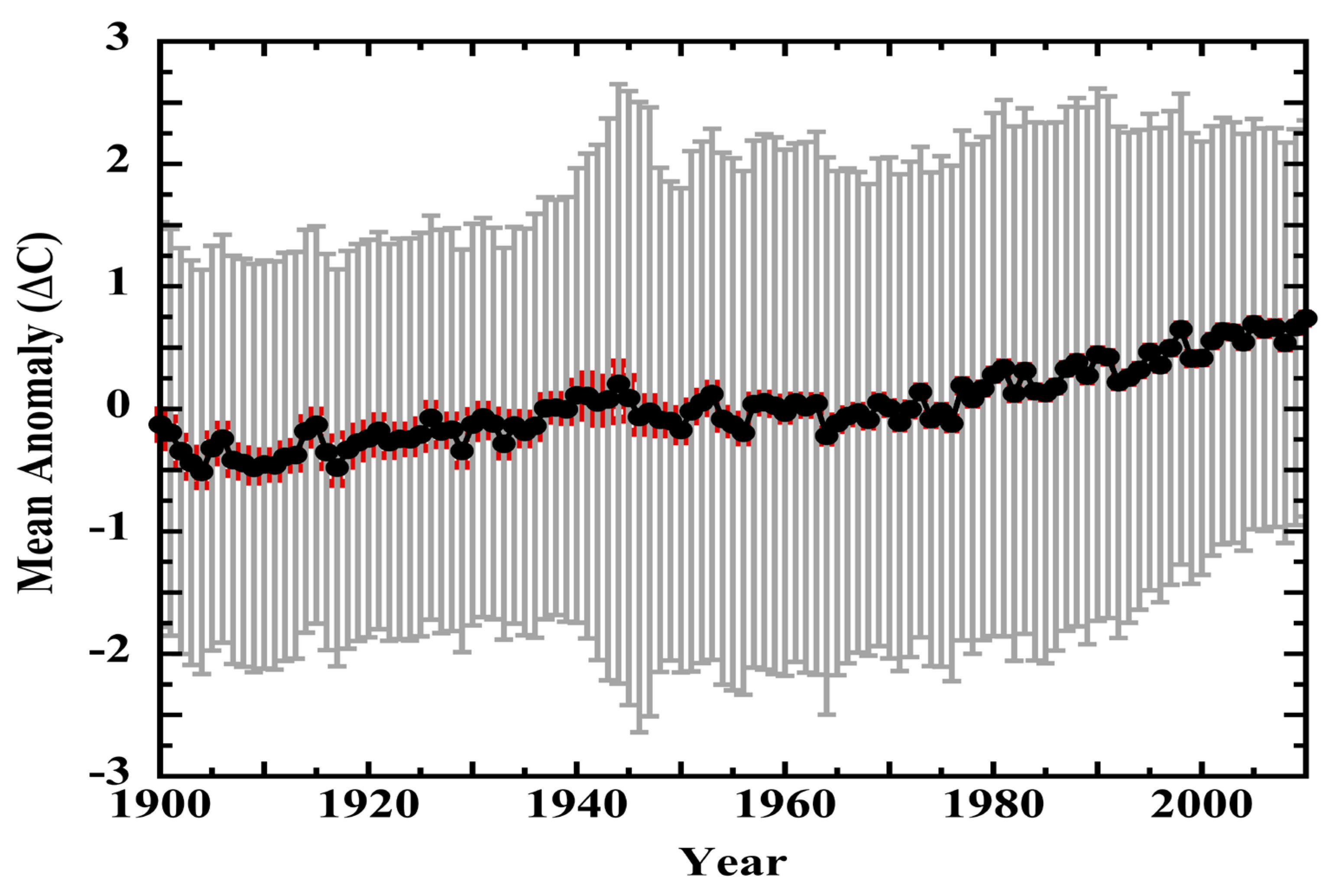
3. Results

3.1. LiG Thermometers: Resolution, Linearity, and Joule-Drift

3.1.1. Resolution

Until relatively recently, the U.S. National Institute of Standards and Technology (NIST) carried out detailed calibrations and evaluations of LiG thermometers [99,100]. NIST publications list the visually indistinct physical imperfections that can degrade the accuracy of a LiG thermometer, including “changes in bulb volume, microscopic alterations in glass geometry at elevated temperature, microscopic cracking, degradation of the thermometer liquid”, and endogenous solids, such as glass particles in the capillary [101,102]. Microscopic inspection to detect such flaws preceded calibration of LiG thermometers at NIST [102]. The presence and influence of physical imperfections that may have affected LiG thermometers over the historical air-temperature-measurement record are unknown.

After about year 2000, NIST calibration and testing of LiG thermometers utilized a computer-driven digital camera and 10× magnification to visualize the meniscus of the liquid column [100,103]. System resolution was 1/34 of the smallest stem division, equivalent to ±0.03 °C for a 1 °C/division LiG thermometer. Under this high-precision visualization, calibration will yield the physical resolution limit of the thermometer. That is, the visualization errors are negligible, leaving calibration errors stemming only from the imperfections and the sensitivity of the thermometer itself.

NIST calibration of two 1 °C/division full-immersion mercury LiG thermometers, with four repetitive readings taken every 25 °C between 0–100 °C, yielded a 2σ = ±0.11 °C (95% CI) resolution limit [100]. The same ultimate 2σ = ±0.12 °C uncertainty was found in an interlaboratory comparative calibration of three 0.1 °C/division full-immersion Hg LiG Thermo-Schneider thermometers [104]. The ±0.12 °C uncertainty emerged despite the fact that the visualization apparatus provided 1/5 (±0.02 °C) division resolution. This 2σ = ±0.11 °C represents the resolution (detection) limit—the lowest limit of uncertainty—that can be associated with a temperature measured using a meteorological surface-station mercury LiG Celsius thermometer. A meteorological LiG air-temperature thermometer may be considered total immersion, as the entire instrument is bathed in ambient air.

Prior to year 2000, LiG thermometer calibrations at NIST employed visualization by eye, which is the standard method used to obtain LiG thermometer readings at meteorological stations. The uncertainty attending a LiG thermometer reading taken by eye (visual repeatability) is 1/4 of a scale division [101,105]. For a calibrated 1 °C/division mercury or alcohol (spirit) meteorological LiG thermometer, the true air temperature is taken to be somewhere within ±0.125 °C of the measurement as read by eye. The reported uncertainty associated with this rectangular probability distribution is 1σ = (±0.125/$\sqrt{3}$) °C = ±0.072 °C. The lower-limit estimate of laboratory accuracy for a visually-read 1 °C/division full-immersion mercury LiG meteorological thermometer combines in quadrature the intrinsic resolution limit plus the repeatability. Thus, 2σ = 1.96 × $\sqrt{{(0.055)}^2+{(0.072)}^2}$ = ±0.178 °C. This is the minimum confidence interval that must condition any meteorological air temperature, or a mean of air temperatures. The ±0.18 °C, 95% lower limit of uncertainty, is the laboratory ideal instrumental-accuracy limit, representing resolution combined with visual repeatability. If a LiG thermometer suffers ice-point calibration drift and is recalibrated, the uncertainty from visual repeatability again enters. For a 1 °C/division LiG thermometer, the new lower limit of uncertainty following recalibration is then 2σ = 1.96 × $\sqrt{{(0.055)}^2+{(0.072)}^2+{(0.072)}^2}$ = ±0.23 °C [101].

In constructing an air-temperature anomaly, both every station mean and the reference normal will each carry, at least, the lower limit ±0.18 °C as the 95% RMS uncertainty. Taking the (mean minus normal) difference to obtain an annual air-temperature anomaly requires combining the respective uncertainties in quadrature [106]. This calculation yields $2\sigma =1.96\times \sqrt{{(\mathrm{0.0.0908})}^2+{(\mathrm{0.0.0908})}^2}$ = ±0.25 °C as the 95% lowest-limit uncertainty bound in any LiG-derived mean air-temperature anomaly.

However, NBS/NIST calibration circulars published between 1911–1994 tabulated the accuracy for calibrated full-immersion mercury LiG thermometers of 1 °C/division to be ±0.1–0.2 °C following correction for all known systematic errors [102,107,108,109]. The tolerance limit—the maximum of error in an uncalibrated thermometer—was ±0.5 °C. Accepting the 1911–1994 NBS/NIST intermediate ±0.15 °C accuracy value for good-quality full-immersion mercury LiG thermometers over the 20th century, along with the standard ±0.072 °C visual repeatability, the lower-limit 95% uncertainty becomes 2σ = 1.96 × $\sqrt{{(0.15)}^2+{(0.072)}^2}$ = ±0.326 °C in both any pre-2000 meteorological air temperature and in the RMS uncertainty of a 30-year air-temperature reference normal. In this case, the 95% lower limit of experimental uncertainty in a pre-2000 mean air-temperature anomaly becomes 2σ = $1.96\times \sqrt{{(0.166)}^2+{(0.166)}^2}$ = ±0.46 °C.

This NIST calibration range of accuracy marks the lower limit of uncertainty for temperatures read from full-immersion mercury LiG meteorological thermometers scaled to 1 °C/division, prior to year 2000. As noted above, NIST automated the visualization for their calibration procedure after 2000 [103], which improved the accuracy of calibration. This greater level of LiG calibration accuracy yields an uncertainty of 2σ = ±0.25 °C in a post-2000 annual LiG temperature anomaly, as noted above. In constructing a global air-temperature anomaly, this uncertainty enters as the weighted fraction of LiG thermometer temperatures.

Table 1. NIST 1 °C/division Mercury LiG Thermometer Calibration Resolution Limits (±2σ, °C).

	Eye Alone	Magnifying Lens
accuracy limit (resolution) a	0.300	0.114
visual repeatability	0.144	0.144
per-measurement uncertainty b	0.326	0.178
anomaly uncertainty c	0.461	0.252

^a Three significant figures are used throughout to reduce round-off error. ^b root–sum–square of resolution and visual repeatability. ^c Uncertainty in an anomaly is the root–sum–square of the uncertainties in the differenced magnitudes.

summarizes the base-level uncertainties conditioning the Hg LiG air temperatures.

The empirical uncertainty of alcohol-filled LiG low-temperature thermometers is about twice that of the Hg LiG instruments [99,102]. The estimated pre-year-2000 ± 2σ uncertainty in an alcohol LiG Celsius thermometer, per measurement, is then ±0.62 °C or is ±0.87 in an anomaly. Post year 2000, the uncertainties are ±0.23 °C per measurement and ±0.32 °C in an anomaly. The same absolute values of resolution and repeatability are applicable to Fahrenheit thermometers, with uncertainties improving by 5/9 over the Celsius LiG instrument. Table 1 lists laboratory resolution limits only. Uncertainties following from non-linearity and Joule-drift (see below) are not included.

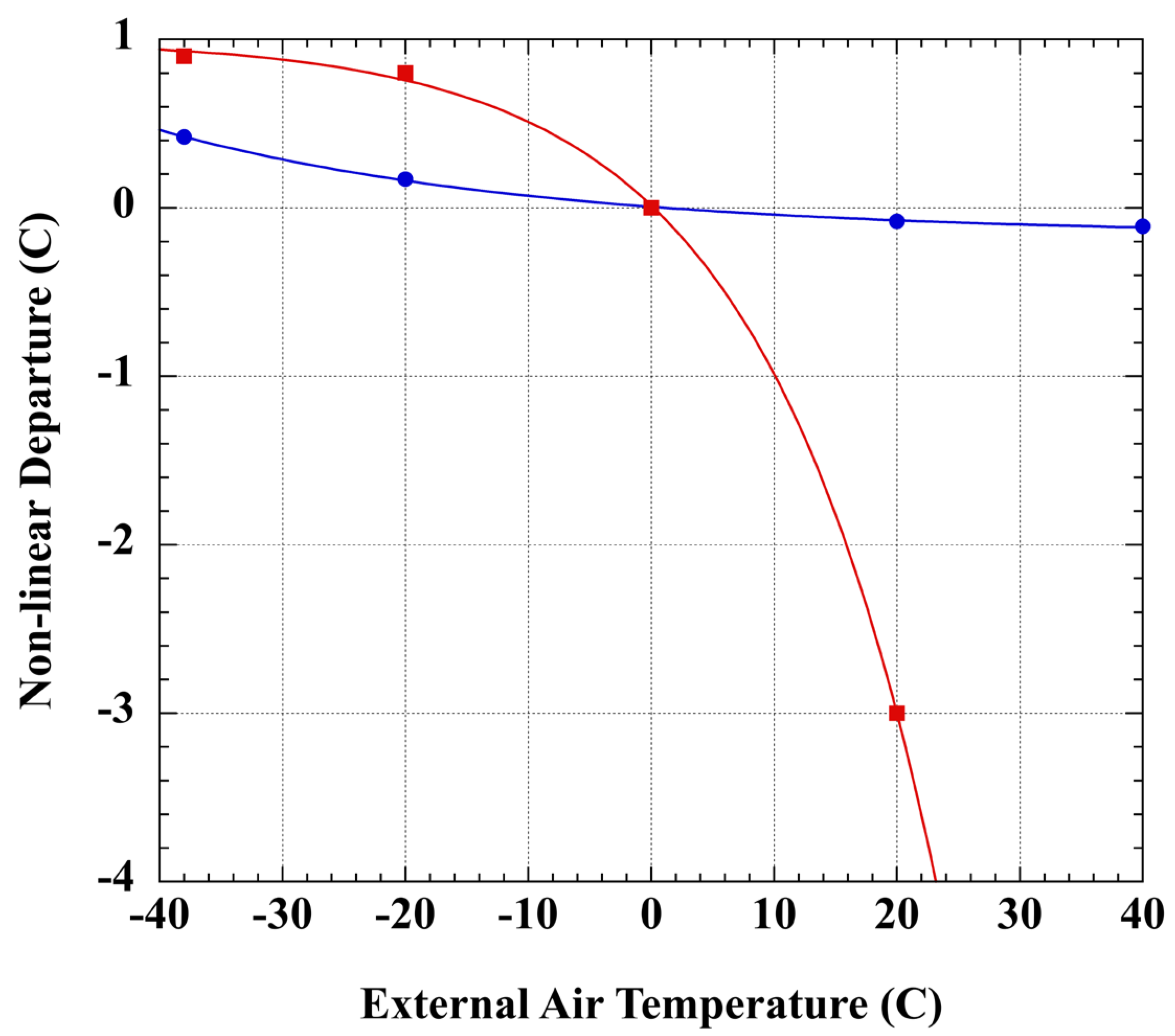
3.1.2. Linearity

Degradations of LiG thermometer resolution due to physical deterioration are episodic and local. However, non-linearity of response is a small but universal source of measurement error in LiG thermometers [93,110]. Non-linearity of LiG thermometers arises because the mercury or ethyl alcohol in the capillary does not expand uniformly with temperature [111,112]. Following two-point calibration at 0 °C and 100 °C, a meteorological thermometer will parabolically depart from the correct temperature above 0 °C and recover at 100 °C, reaching a maximum of error near 50 °C [110,112,113].

Figure 1 shows these errors over the range of meteorological temperatures. For mercury thermometers, the error is relatively small, however, error can be significant in spirit thermometers. The World Meteorological Organization does not include non-linearity among the errors specific to spirit thermometers [114]. Assuming alcohol LiG thermometers dominate the historical daily minimum temperature record, and mercury LiG instruments the daily temperature maxima, then from Figure 1 any uncorrected minimum temperatures in Winter will have been recorded as too warm and in Summers as slightly too cool. For example, an uncorrected single Winter day of −10.00 °C minimum (alcohol) and 10.00 °C maximum (Hg) temperatures, corrects to −9.49 °C and 9.96 °C, respectively. The nominal 0 °C average thus corrects to 0.24 °C.

Although the correction is modest, the error due to non-linearity of response is present in the historical LiG air-temperature measurements entering the global average. Correction of this error is not mentioned in published work. The larger relative magnitude of the alcohol correction implies a slightly warmer past than presently recognized, which should be considered in estimates of climate warming. Correction of past temperatures for non-linearity of response requires knowing the characteristics of the land-surface-station and ship-borne LiG thermometers.

3.1.3. Joule-Drift

The slow upward drift in ice-point calibration temperature due to contraction of the glass bulb of a LiG thermometer was first reported in 1808 [112]. A detailed investigation of this problem was reported in 1837. Bulb contraction in LiG thermometers occurs because residual strain remains in the glass after manufacture. As this strain is slowly released the bulb contracts, which, in turn, causes the indicating liquid to rise in the stem. An artifactual increase in measured temperatures is thereby produced [112,115,116]. Mid-19th century thermometer recalibrations after decades to centuries of use revealed ice-point calibration shifts of 0.3–0.6 °C due to bulb contraction [112,115,117]. Left uncorrected, bulb contraction in early meteorological LiG thermometers will have produced a false warming trend extending across decades.

The changes in volume of LiG thermometer bulbs came under detailed examination in the mid-19th century and continued well into the 20th [94,117,118,119,120,121,122,123,124,125,126,127]. Starting in April 1844, James Joule began an ice-point drift experiment using a long high-resolution Dancer Hg-LiG Fahrenheit thermometer that had been manufactured a few months earlier. Joule performed 13 ice-point temperature calibrations on this thermometer through to December 1882 [95,128]. By that time, it was common knowledge that ice-point drift was inevitable and that the relaxation behavior of each thermometer was unique [117,125,129]. Following Joule’s death in 1889, three more ice-point calibrations were obtained on the same Dancer thermometer during 1892–1894 [130]. The final calibration was performed in 1930, by which time the departure was 0.67 °C [131,132]. Unfortunately, the glass composition of Joule’s Dancer thermometer is unknown and the thermometer itself was lost in 1942 during a WWII air-raid.

Sydney Young first reported that the rise in ice-point temperature in Joule’s LiG thermometer was exponential with time [94]. Young’s finding was later grounded in physical theory [121]. The upward drift in LiG thermometer ice-point temperatures was found to follow one or more relaxation processes, T = a(1 − e^−kt), where T is temperature, a is a constant, k is a rate constant, and t is time in years [118].

Figure 2 shows the 86 years of measurement creep in Joule’s Dancer thermometer. The points were fit with two Taylor–Noyes exponentials [118]. These imply at least two independent relaxation mechanisms within the bulb-glass, with half-lives of 1 ± 0.2 year and 18 ± 2 years. Thus, about 180 years (10 half-lives) are required for the secular change in the Dancer bulb volume to become negligible. The more rapid process diminishes to about 3% of its initial rate after 5 years. This explains the confidence among 19th century manufacturers and researchers in the accuracy of thermometers that had been calibrated a few years after filling. However, Figure 2 indicates this confidence was misplaced. Joule’s ice-point measurements have been investigated extensively [133,134,135,136]. However, the two exponential phases shown in Figure 2 were not resolved.

Prior to 1885, thermometers were manufactured from glasses typified by “Thuringian” glass (Table 2), or from lead (PbO, litharge) glass, each of which contained significant fractions of both sodium and potassium ions. Nineteenth-century lead-glass thermometers exhibited an increased rate of bulb contraction [125,137,138,139,140]. Following the discovery of bulb-contraction, the most careful manufactories scored and calibrated their LiG thermometers several months after being filled and sealed [112]. After about 1880, Kew Observatory manufacture of LiG thermometers included heating in an oil bath for 2–3 weeks prior to calibration, and at a temperature exceeding the limit of measurement [141]. However, these were only partial solutions, because, even after treatment at elevated temperature, ice-point drift could continue for decades at ambient temperature (cf. Figure 3).

In 1884 Otto Schott and Ernst Abbe traced bulb contraction to the mixed alkali effect (MAE), i.e., glass compositions that included significant fractions of both potassium and sodium oxides [123,124,142,143,144,145,146,147]. Their Jena hard glass 16^III and 59^III, manufactured after 1885, introduced B₂O₃ into thermometer glass. The new process simultaneously excluded lead oxide and restricted alkali metal usage to Na₂O. These compositional adjustments reduced bulb contraction and thermometer ice-point drift by about 10-fold. The molecular mechanism of bulb stress relief includes movement and polymerization of silicate ions [148]. The mechanistic dynamics are complex and remain an open area of research [142,145,148,149,150,151].

Figure 3 illustrates the dramatic difference of lead-glass (Corning 0041) versus hard borosilicate glass (Corning 1720) in thermometer-bulb contraction. Each exhibits a faster and slower process. After 360 days at 262 °C, the lead-glass thermometer exhibited a ~14-fold greater shift in ice-point. Table 2 presents representative glass compositions of LiG thermometers exhibiting the different behaviors.

Figure 3. (points), mercury LiG thermometer ice-point drift measured during roasting at 262 ± 1 °C [122]. The blue fitted line is the sum of two Taylor–Noyes exponentials [a × (1 − e^−kt)] [118]. (a) Corning 0041 potash–soda–lead–silica glass [152]; (red), a₁ = 0.34 ± 0.01, k₁ = 0.22 ± 0.02 d⁻¹, t^1/2 = 3 d; (green), a₂ = 0.57 ± 0.02, k₂ = 0.0056 ± 0.0007 d⁻¹, t^1/2 = 119 d, r² = 0.996. (b) Corning 1720 borosilicate glass [153]; (red), a₁ = 0.027 ± 0.001, k₁ = 0.48 ± 0.09 d⁻¹, t^1/2 = 1.4 d; (green), a₂ = 0.033 ± 0.001, k₂ = 0.010 ± 0.001 d⁻¹, t^1/2 = 70 d; r² = 0.989.

Figure 3. (points), mercury LiG thermometer ice-point drift measured during roasting at 262 ± 1 °C [122]. The blue fitted line is the sum of two Taylor–Noyes exponentials [a × (1 − e^−kt)] [118]. (a) Corning 0041 potash–soda–lead–silica glass [152]; (red), a₁ = 0.34 ± 0.01, k₁ = 0.22 ± 0.02 d⁻¹, t^1/2 = 3 d; (green), a₂ = 0.57 ± 0.02, k₂ = 0.0056 ± 0.0007 d⁻¹, t^1/2 = 119 d, r² = 0.996. (b) Corning 1720 borosilicate glass [153]; (red), a₁ = 0.027 ± 0.001, k₁ = 0.48 ± 0.09 d⁻¹, t^1/2 = 1.4 d; (green), a₂ = 0.033 ± 0.001, k₂ = 0.010 ± 0.001 d⁻¹, t^1/2 = 70 d; r² = 0.989.

Both Joule’s Dancer thermometer (Figure 2) and the two test thermometers (Figure 3) indicate similar simultaneous fast and slow relaxation processes. The modern lead–silica LiG thermometer produced the expected larger and more extensive ice-point drift. The improvement realized in a borosilicate glass LiG thermometer is evident in the 14-fold reduction in ice-point drift at 360 days.

The glass composition of Joule’s Dancer thermometer is unknown. The notion that it was the borosilicate of Jena glass 59^III is not tenable [134,136]. Jena borosilicate glasses were not developed until 1885 [123,143], 41 years after Joule acquired his thermometer. Although William Harcourt experimented with borosilicate glass in the mid-19th century, his focus was on optical instruments [123,154]. B₂O₃ was not used in thermometer glass until after the experiments of Schott and Abbe at the Jena glassworks in 1883–1884 [123,143]. The new Jena 59^III borosilicate glass produced thermometers with a greatly diminished ice-point drift, which is inconsistent with the 0.67 °C drift exhibited by Joule’s Dancer thermometer. The Joule thermometer drift is consistent with lead–silica glass (compare Figure 2 with Figure 3a vs. Figure 3b), which was in general use for thermometers in the mid-19th century. For example, a Scottish scientific thermometer dating from the first decades of the 19th century was composed of glass containing 20.2% PbO [140].

Table 2. Relevant Thermometer Glass Compositions.

Glass Type	SiO2	Na2O	K2O	CaO	B2O3	Al2O3	PbO	Reference
Silica-lead a	68	10	6	1	---	---	15	[152]
Borosilicate a	80	14	---	---	14	2	---	[152]
Corning 0041	50.1	6.6	1.5	---	---	1.9	39.9	[155]
Corning 1720 b	62	1	---	8	5	17	---	[153]
Jena 59III c	72	11	---	---	12	5	---	[156]
Thuringian d	68.7	15.9	7.3	5.7	---	2.1 e	---	[144]
Kew f	53.9	1.7	8.5	0.56	---	0.48	34.5	[157]
Kew g	53	0.5	11.5	---	---	0.5 d	34	[158]

^a Representative compositions. ^b Includes ~7% MgO [159]. ^c Single alkali reduces thermometer bulb contraction. ^d Typical of German and French common thermometer glass prior to 1885; included ~0.24% MgO. ^e May also include Fe₂O₃. ^f From the early 1850′s; mean of analyzed percentages in ref. [160]; included traces of Fe₂O₃ and MnO. ^g Introduced around 1880 [139].

Table 2. Relevant Thermometer Glass Compositions.

Glass Type	SiO2	Na2O	K2O	CaO	B2O3	Al2O3	PbO	Reference
Silica-lead a	68	10	6	1	---	---	15	[152]
Borosilicate a	80	14	---	---	14	2	---	[152]
Corning 0041	50.1	6.6	1.5	---	---	1.9	39.9	[155]
Corning 1720 b	62	1	---	8	5	17	---	[153]
Jena 59III c	72	11	---	---	12	5	---	[156]
Thuringian d	68.7	15.9	7.3	5.7	---	2.1 e	---	[144]
Kew f	53.9	1.7	8.5	0.56	---	0.48	34.5	[157]
Kew g	53	0.5	11.5	---	---	0.5 d	34	[158]

^a Representative compositions. ^b Includes ~7% MgO [159]. ^c Single alkali reduces thermometer bulb contraction. ^d Typical of German and French common thermometer glass prior to 1885; included ~0.24% MgO. ^e May also include Fe₂O₃. ^f From the early 1850′s; mean of analyzed percentages in ref. [160]; included traces of Fe₂O₃ and MnO. ^g Introduced around 1880 [139].

3.2. Lead Glass

In the early 1850s, the Kew observatory purchased a lead glass (Choisy le Roi crystal [161]) thermometer from Paris chemist and instrument-maker Henri Regnault for use as a standard applied to their own manufacture of thermometers [157]. From this mid-19th century start, Kew Observatory came to supply high-quality standard thermometers composed, bulb and stem, of glass with ~34% lead oxide (Table 2) to European and American experimenters [139,158]. E. H. Griffiths mentioned that soft-glass thermometers were in wide English use as late as 1894 [162]. During the late 19th century, both lead glass and hard glass were used in manufacture of thermometers by Tonnelot and his successor Baudin in Paris [117,162,163]. However, by 1903 Baudin moved to lead-free French hard glass (verre dur) [110,164].

Figure 4 shows the Pb L-edge X-ray fluorescence (XRF) spectrum of the bulb glass of a Baudin meteorological LiG spirit thermometer, manufactured around 1900 and purchased by the U.S. Weather Bureau (see Facilities and Methods).

The noise intensity of the Pb L-edge XRF spectrum is within the width of the line, indicating considerable lead. This thermometer was purchased by the U.S. Weather Bureau in 1902, and donated to the National Museum of American History in 1960. Thus, lead-glass meteorological LiG thermometers continued to be manufactured and brought into service as late as 1900.

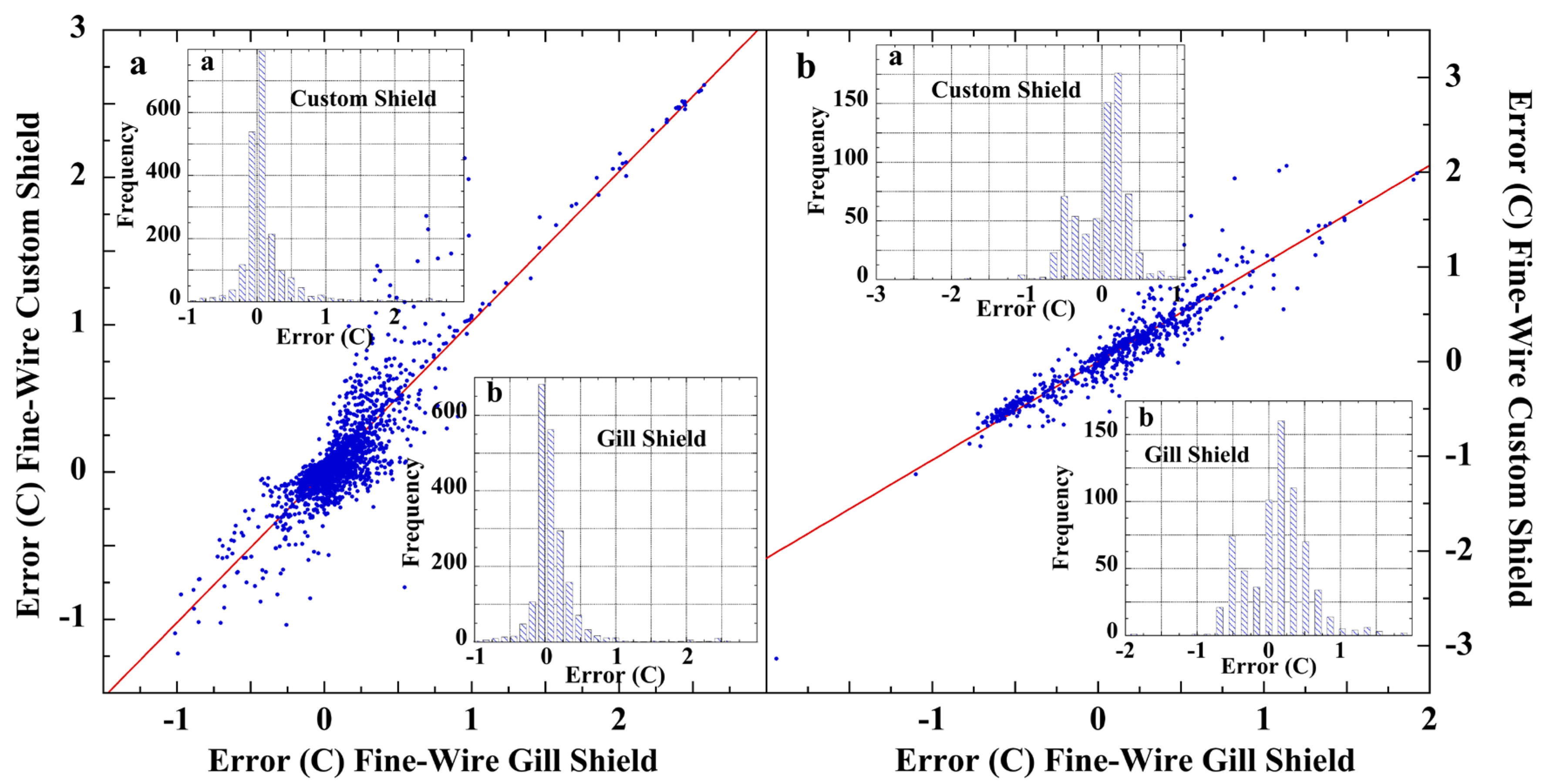
3.3. Thermometer Field Calibration and Measurement Error

Field-calibration experiments of naturally ventilated temperature sensors at surface weather stations reveal systematic measurement errors, due primarily to the uncompensated common environmental variables of solar irradiance, surface albedo reflectance, and insufficient wind speed [6,8,31,33,41,165,166,167]. The systematic measurement error due to uncompensated environmental variables is examined next.

3.3.1. De Bilt (Netherlands)

Brandsma and van der Meulen reported extensive field-calibration experiments using platinum resistance thermometer (PRT) sensors mounted within nine naturally ventilated louvered sensor shields of varying configurations [168,169]. Air-temperature-measurement differences were calculated relative to a naturally ventilated KNMI multiplate reference. All the screens were equipped with PRTs of identical make. Thus, measurement errors are restricted to the impact of the shield. In general, the mean seasonal differences with respect to the KNMI reference was ≤0.1 °C. However, the question addressed here is measurement accuracy, rather than inter-screen means.

The test shields included two naturally ventilated Stevenson screens of KNMI design; one constructed of wood and the other of polyvinyl chloride (PVC). These are of particular interest because LiG thermometers housed in Stevenson screens have provided the great bulk of historical land-surface air temperatures [170]. Figure 5 shows the frequency distribution histograms of the (T_Stev. minus T_KNMI) temperature-measurement errors obtained within the wood or PVC Stevenson screens.

The error distributions are neither normal nor comparatively equivalent, and are biased warm. The overall error frequency maxima (f_m) and RMS errors are similar (0.00 °C and 0.01 °C, resp.; RMS = ±0.2 °C). An adequate fit to each distribution required the combined intensities of a Lorentzian and two Gaussian lines (

Table 3. Fit Parameters for Stevenson Shield Calibration Error.

	Gaussian 1 (fm, σ)	Gaussian 2 (fm, σ)	Lorentzian (fm, Γ)	Fit r2
Stev. (Wood)	0.108, 0.230	0.024, 0.096	2 × 10−4, 0.084	0.999
Stev. (PVC)	0.041, 0.172	8.3 × 10−3, 0.052	−0.029, 0.036	0.943

). These line shapes do not necessarily reflect physically real processes, but, rather, indicate the structural complexity of the measurement error. Although the fitted line shapes in each histogram are analogous, the intensities, FWHM, and offsets are disparate. Each screen was subjected to virtually identical external variables of wind speed and irradiance, but produced different internal thermal environments. The measurement errors clearly change with material state, as the screens were dimensionally equivalent.

A correlation plot of the calibration-error data sets for the wooden and the PVC Stevenson screens (Figure 6) shows correlation r = 0.92, which strongly disconfirms the universal assumption of random measurement error in air-temperature measurements. Analogous calibration error histograms and correlation plots for the De Bilt Socrima, R. M. Young, and Vaisala screens are shown in Figure S1 of the Supplementary Materials.

Mean pair-wise correlations of systematic error were assessed for all the experimental screens of the Brandsma–van der Muelen test series (

Table 4. KNMI Average Correlations of Test-Screen Temperature Error 1989–1995.

	Socrima	Young Gill	Stv. PVC	Stv. Wood	Stv. PVC asp	Vaisala	Young asp II	KNMI asp
Socrima	1	0.28	---	0.64	0.14	0.18	0.15	0.30
Young Gill		1	0.33	0.28	0.27	0.54	0.32	0.60
Stv. PVC			1	0.88	---	0.30	---	0.07
Stv. Wood				1	0.04	0.18	0.06	0.17
Stv. PVC asp					1	0.28	0.47	0.36
Vaisala						1	0.44	0.76
Young asp II							1	0.35
KNMI asp								1

Average correlation is the RMS positive root. Some screens had no measurement-overlap periods. All screens were naturally ventilated, except those marked ‘asp’.

). Five pairs show error correlation r ≥ 0.5 and another 12 show r ≥ 0.25.

Significant screen-pair correlations of systematic error are also evident year-by-year over the seven-year test period, shown in Tables S1–S7 in the Supplementary Materials. The six-year composite r = 0.88 of the Stevenson screen pair was the strongest correlation of measurement error. This is especially relevant because the historical land-surface air-temperature record is dominated by LiG thermometers housed in Stevenson screens.

3.3.2. Plaine Morte Glacier (Swiss Alps)

Huwald and associates installed a meteorological station on the Plaine Morte Glacier in the Swiss Alps (2700 m mean altitude) [36].

Test temperature sensors included a PRT mounted within a naturally ventilated R.M. Young multiplate shield and a fine-wire thermocouple. These instruments were calibrated against a sonic anemometer air-temperature reference, which is insensitive to irradiance and wind-speed effects.

The naturally ventilated R.M. Young multiplate shield and the fine-wire thermocouple exhibited significant calibration errors; ε_calib = 2.2 ± 1.9 °C and ε_calib = 1.9 ± 1.1 °C, respectively. The correlation plot, Figure 7, yielded sensor-calibration measurement error correlation r = 0.86. The error-frequency histograms (Figure 7, insets) show that each error set strongly departs from a normal distribution. Shapiro–Wilk tests for normality yielded: fine-wire thermocouple error, W(1154) = 0.941, p < 0.001; and PT100 thermistor error, W(1155) = 0.959, p < 0.001, indicating non-normal distributions and confirming the visual appraisal.

3.3.3. HOBO Thermistors, Ottawa

Mauder and associates reported a calibration of 25 air-temperature sensors, each consisting of a thermistor housed in a naturally ventilated multiplate HOBO shield [90]. The reference temperature-measurement standard was a high-accuracy thermistor housed within a fan-aspirated radiation shield.

The 25 HOBO sensors were arranged in a 5 × 5 grid situated in a 10 m × 10 m area. The reference thermistor was located 2 m away from one corner of the grid. Calibration air temperatures were measured during 2–3 May 2007. Calibration error for each HOBO sensor is the temperature-measurement difference with the aspirated reference sensor. Figure 8 displays the calibration error mean of HOBO #2 through HOBO #25 plotted against the error produced by the HOBO #1 thermistor.

The very high r = 0.94 correlation of HOBO #1 error with the 24-average is pair-wise repeated for the entire set of 25 HOBO sensors. The highly non-normal error distribution (Figure 8, inset) is likewise evident in each of the 25 HOBO error series (Figure S2 in the Supplementary Materials). Table S8 in the Supplementary Materials provides RMS calibration error for all 25 HOBO shields, the individual pair-wise inter-sensor error correlations, and the results of Shapiro–Wilk tests for normality. The HOBO error means and calibrations are highly correlated (r = 0.97, Figure S3 of the Supplementary Materials), indicating that the 25 HOBO shields produced very similar measurement errors in response to heating from irradiance and insufficient wind speed. The combined HOBO error set (N = 54,000) exhibited a non-normal distribution (Figure S4 in the Supplementary Materials), all of which again disconfirm the notion of random measurement error.

3.3.4. Wire Thermocouples, SRNL

An extensive field test of fine-wire thermocouple temperature sensors was carried out in 2008 at the Savannah River National Laboratory [171]. The purpose was to test the accuracy of air-temperature measurements using sensors housed in unaspirated shields. Two reference sensors included a fine-wire thermocouple and a platinum resistance thermometer (PRT) each housed in a Yankee MetOne-2010 aspirated shield and accurate to ±0.1 °C. The two test sensors were fine-wire thermocouples, with one in a naturally ventilated Gill shield and the other within a naturally ventilated custom multi-plate shield having the same spacings as the test Gill shield. Figure 9 shows that highly correlated measurement errors were produced by the two naturally ventilated fine-wire sensors, when differenced against either of the two aspirated reference sensors.

In Figure 9, the error distributions and the mean magnitudes varied with the aspirated calibration sensor (

Table 5. Measurement Error in Naturally Ventilated Fine-Wire Thermocouple Sensors.

Aspirated Ref. →	Thermocouple Yankee 2010		PRT MetOne 327-C
Test shield ↓	Error (µ ± σ; °C)	Shapiro–Wilk	Error (µ ± σ; °C)	Shapiro–Wilk
Gill (N = 2072)	0.11 ± 0.34	0.696, p < 0.001	0.12 ± 0.45	0.968, p < 0.001
Custom (N = 691)	0.11 ± 0.40	0.701, p < 0.001	0.12 ± 0.49	0.945, p < 0.001

Data are from the Savannah River National Laboratory calibration experiment [171].

). This disparity was assigned to air-flow differences, with the aspirated thermocouple yielding the more accurate calibration [171]. Nevertheless, each calibration sensor revealed that the naturally ventilated screens produced correlated systematic measurement errors. The Shapiro–Wilk test (Table 5) indicated the measurement errors were non-normal. Similar correlated or non-random errors were found in other co-located air-temperature sensors, including those on a floating buoy, as shown in Figures S5–S8 and Table S9 in the Supplementary Materials [67].

All the examined calibration-experiment error sets revealed a warm bias and a non-normal distribution. Additional calibration experiments, not discussed here, have yielded similar air-temperature-measurement uncertainties that invariably arise with the use of naturally ventilated shields [34,35,44,45,68]. A high-quality Siemens thermistor housed in a naturally ventilated Stevenson screen produced a non-normally distributed measurement error (N = 144) (Figure S9 in the Supplementary Materials)) [35]. In the same experiment, copper–Constantan wire thermocouple sensors produced highly correlated air-temperature-measurement errors. Likewise, calibration of a PRT housed in a MetSpec double-louvered plastic Stevenson screen produced a non-normal distribution of systematic measurement error (N = 81,504) (Figure S10 of the Supplementary Materials) [45].

Table 6. RMS Calibration Measurement Uncertainty within Naturally Ventilated Shields.

Sensor Shield	Uncertainty (±°C)	Calib. Sensor	Reference
Stv. Wood a	0.20	asp. PRT b	[168]
Stv. PVC a	0.19	asp. PRT	[168]
HOBO (25 avg) c	0.43	asp. PRT	[90]
CRS d	0.53	asp. PRT	[31]
MMTS e	0.25	asp. PRT	[31]
MMTS f	0.28	asp. thermistor	[32]
Gill g	0.26	asp. PRT	[31]
Gill h	0.45	asp. PRT	[171]
Custom Plate h	0.49	asp. PRT	[171]
Gill h	0.36	asp. Therm. i	[171]
Custom Plate h	0.40	asp. Therm. i	[171]
Thermocouple k	2.20	Sonic Anem. j	[36]
R. M. Young k	2.95	Sonic Anem. j	[36]
MMTS k,l	0.31	asp. CRN m	[172]
Stv. Wood (lg)	0.24	asp. PRT	[68]
Stv. Wood (sm)	0.23	asp. PRT	[68]

^a Wooden or polyvinylchloride Stevenson screen. ^b aspirated platinum resistance thermometer. ^c Average of 25 naturally ventilated shields. ^d Cotton region shelter. ^e Min–max temperature system. ^f over a snow-covered surface. ^g PRT, Gill plate shield. ^h thermocouple. ⁱ aspirated thermocouple wire. ^j sonic anemometer. ^k Over a snow-covered surface at 2700 m on Alpine Plaine Morte Glacier, Switzerland. ^l December–February day–night average error scaled to reflect 10 daylight hours at Lincoln, NB, USA (40°48′00″ N; 96°40′00.012″ W). ^m Standard Climate Research Network aspirated shield.

lists the uncertainties due to systematic measurement error as produced by naturally ventilated shields during the several field-calibration experiments described above.

The full KNMI field-calibration experiments (Section 3.3.1) permit a test of the distribution produced by multi-sensor cumulated measurement errors in the land-surface global air-temperature record [167,168,169]. This field test consisted of five naturally ventilated PRT sensors, including two Stevenson screens (constructed from wood or PVC), and Visalia, Socrima, and T. Young multiplate shelters. Each screen was exposed to at least two years of varying weather, across the six years of the field calibration (January 1989–February 1995). The large sample size, varying weather, and multiple screen types in combination provided a valid test of the assumption of strictly random errors in land-surface temperature measurements. The assumption requires that a large varied error data set produces a normal distribution.

For this test, the complete set of (sensor minus KNMI reference) calibration errors from all five sensors were appended into a single file (N = 667,403). Figure 10 shows a histogram of the combined error data points, which was well fitted with a Lorentzian line-shape. A Gaussian fit (Figure S11 in the Supplementary Materials) was notably deficient at the wings. The near-Lorentzian distribution and the evidence of correlated error strongly disconfirm the notion of random measurement error.

3.4. Sea-Surface Temperature

Categorical sea-surface temperature (SST) can be divided into T_t, the physically correct (true) temperature of the in situ waters, T_s, the temperature of an acquired water sample, and T_m, the measured temperature. T_t is generally unknown absent in situ measurement using a high-accuracy, high-precision temperature sensor. Under ideal circumstances, T_s ≈ T_t within sampling integrity, and T_m ≈ T_s within the accuracy limit of a standard sensor—historically, a LiG thermometer or, less often, a thermistor—and given care in measurement protocol. For example, a U.S. Naval study of the reliability of expendable bathythermograph (XBT) measurements, carried out by trained personnel reported LiG thermometer bucket SSTs to be within 0.01 ± 0.1 °C of the measurements of a highly accurate conductivity/depth/temperature (CDT) sensor [173].

3.4.1. Context

Shipboard measurements prior to year 1990 contributed the great bulk of sea-surface temperatures (SSTs) entering the International Comprehensive Ocean–Atmosphere Data Set (ICOADS) [174,175,176,177,178]. The ICOADS compilation is used in the construction of the global air-temperature record [13,55,59,72,75,179]. The great bulk of shipboard SST measurements utilized LiG thermometers to measure the temperature of either engine-intake water or of a seawater sample drawn up onto deck using a specialized meteorological bucket [75,176,180]. The accuracy of the historical measurements is under examination here.

The sources and estimates of measurement errors attending bucket and engine-intake SSTs have been thoroughly discussed elsewhere and will not be reiterated here [74,75,79,80,82,84,181,182,183,184].

The limits of resolution and non-linearity specific to LiG thermometers, described in Section 3.1.1 and Section 3.1.2 above, apply equally to LiG thermometers used to measure sea-surface temperature (SST) from bucket samples and ship-engine-intake water. Likewise, the uncertainty due to Joule-drift will apply to those SSTs measured using LiG thermometers manufactured prior to 1890.

Compilations of the global SST record are presently conducted under the assumption that the measurement error on each ship (platform) takes a random distribution about a constant ship mean error, relative to the physically correct SST. The global set of ship error means is further assumed to be randomly distributed [71,73,185]. These assumptions persist despite published reports that SST measurement errors vary with the ship, with the cruise, and with the crew [79,80,81]. Nevertheless, the historical SST measurement errors are assumed to coalesce into a normal distribution about their global average mean error offset, which can be removed by differencing. This, in turn, is taken to justify reducing global mean SST measurement error, ±σ_m, by 1/$\sqrt{N}$ in the global record, rendering SST measurement uncertainty insignificant.

3.4.2. Does Semivariogram Analysis Yield the SST Measurement Error Mean?

The semivariogram regression has been used to extract the mean of measurement error from the historical SST record [71,185,186,187]. With subtraction of the derived global mean offset, the residuum of error is assumed to be a normal distribution with a mean of zero and a final negligible uncertainty determined as ±σ/$\sqrt{N}$.

The variogram method is derived from Geostatistics and is used to examine the behavior of paired observables in a spatial field [188,189]. Differences in the magnitude of some set of field observables ‘x’ (e.g., soil pH) are assumed to depend only on the separation distance, typically ‘h’. The variogram tracks the square of the differences:

$$2\gamma \left(h\right)={[\left(x+h\right)-\left(x\right)]}^2,$$

(1)

where x + h is the measurement magnitude of observable x at a distance h from any reference measurement of x, and [(x + h) − (x)]² → 0 as h → 0. Squaring ensures that 2γ(h) is always positive as h → 0. If, on the other hand, 2γ(h) ≠ 0 at h = 0, then the ordinate offset, termed the nugget, derives from measurement error, ε_m, plus microscale variability, c_MS [188]. Kent and colleagues (cited above) used semivariogram analysis, ½[2γ(h)], to appraise pairs of historical SSTs that had been simultaneously measured on spatially separated ships, with the inter-ship distance ranging from proximate to 300 km [71,186]. Microscale SST variability, c_MS, was set to zero at closest proximity. Thus, [(SST₁) − (SST₂)]² regressed against ship-separation distance (h) yielded the nugget at h = 0 as a positive offset. The nugget was taken to be twice the variance of ship-measurement error global mean, and $\frac{1}{2}\sqrt{nugget}=\pm {\epsilon }_m$. Semivariogram analysis was, likewise, used to estimate the error mean in historical marine wind-speed measurements [190].

Examining this usage, any SST measurement T_m = T_t + ε_m, where T_t is the physically correct (true) temperature of the in situ ocean water and ε_m is the combined systematic and random measurement errors. In any such measurement, T_t and ε_m are completely convolved. The correct magnitude of either quantity is not known. When two ships are spatially separated, SST_t1 ≠ SST_t2 and SST_m1 − SST_m2 = (T_t1 + ε_m1) − (T_t2 + ε_m2) = ΔT_t1,2 + Δε_m1,2. When h = 0, T_t1 = T_t2, ΔT_t1,2 = 0, and SST_m1 − SST_m2 = Δε_m1,2. Thus, variogram SST analysis regresses the convolved (ΔT_t1,2 + Δε_m1,2)² against h, and the nugget offset at h = 0 is (Δε_m1,2)² because ΔT_t1,2 = 0. That is, the variogram nugget is the square of the estimated mean difference in error, not the square of the estimated mean error.

In constructing the semivariogram from the variogram, this nugget has been divided by two on the grounds that it represents the mean error of two ships [186,190]. However, as the nugget is, in fact, a difference of errors, dividing by two is incorrect; a difference of one ship has no discrete meaning. Thus, the $\sqrt{{(nugget)}^2}=\sqrt{{(\mathsf{\Delta }{\epsilon }_{m1,2})}^2}=\pm \mathsf{\Delta }{\epsilon }_{m1,2}$ is the estimated root–mean–square (RMS) of the SST measurement error difference mean. It is not the estimated RMS of the SST measurement error mean itself. The magnitude of the SST error mean itself remains unknown. Only the mean difference is revealed. Thus, the mean error of historical ship SST measurements itself remains unknown (and likely unknowable). Homologously, variogram analysis of the marine-wind-measurement error yielded the mean error difference, not twice the error mean [190]. The argument, thus, requires revision.

3.4.3. Are SST Measurement Errors Random?

Instrumental Calibration

The assumption of random error covers the methodologically independent sets of LiG SST measurements arising from buckets or engine-intakes. Field calibrations of bucket and engine-intake SSTs were carried out by Charles Brooks aboard the R. M. S. Empress of Britain cruise ship and aboard the oceanographic research ship C.F.A.V. Endeavor [79,81,191].

The tin-bucket reference thermometer used by Brooks was graduated in 0.5 °C divisions and calibrated as accurate to ±0.2 °C [192]. The R.M.S. Empress of Britain engine-intake thermometer was also scored to 0.5 °C and estimated to be of ±0.3 °C precision. In the later experiments aboard the C.F.A.V. Endeavor as reported by Tabata, a salinity–temperature–depth (STD) recorder, accurate to ±0.02 °C, provided the calibration-reference temperatures. The results of the Brooks and the Tabata calibration experiments are displayed in Figure 11.

The error distribution of measurements acquired aboard the C.F.A.V. Endeavor research vessel (Figure 11c) shows that bucket SSTs can be accurate to ±0.2 °C in the hands of trained personnel [81,191]. On the R.M.S. Empress of Britain, however, bucket error was much larger and varied with the watch; an outcome also noted by Saur (cf. 4-Saur below). Visual inspection indicates their divergence from Gaussian distributions.

Each of the engine-intake calibrations yielded a bias and uncertainty of 0.3 ± 1.2 °C (1σ), which obviates accuracy. Tabata rejected engine-room heat as the source of positive bias because a large fraction of readings was lower than the STD reference temperature. Instead, he assigned the ±1.2 °C standard deviation to reading error. However, carelessness in thermometer reading by professionals and crew aboard a meteorological-research vessel does not seem likely.

Nevertheless, the ship bucket and engine-intake measurement errors displayed non-normal distributions, inconsistent with random error. These calibration outcomes are tested more widely below.

The Difference of Normal Distributions

The assumption of random measurement error is subject to a general test. Any normally distributed data set X = [x₁, x₂, … x_n] can be expressed in its standardized form, Z = (X − µ)/σ, where Z = [z₁, z₂, … z_n] are real numbers and each x_i is z_i standard deviations away from µ [194]. Rearranging, X = Zσ + µ and the difference between two normally distributed data sets is X₂ − X₁ = ΔX_2,1 = (Zσ₂ + µ₂) − (Zσ₁ + µ₁) = Z($\sqrt{\left({\sigma }_2^2-{\sigma }_1^2\right)}$ + (µ₂ − µ₁). Then ΔX_2,1 = ZΔσ_2,1 + Δµ_2,1 and the distribution of the differences is Z = (ΔX_2,1 − Δµ_2,1)/Δσ_2,1. Thus, the difference of two normal distributions is another normal distribution. If the respective canvas bucket and engine-intake SST measurement errors are normally distributed, therefore, their difference set should be normally distributed. This approach has the advantage that error distributions can be illuminated through error difference sets, without needing to know the errors themselves. This test follows.

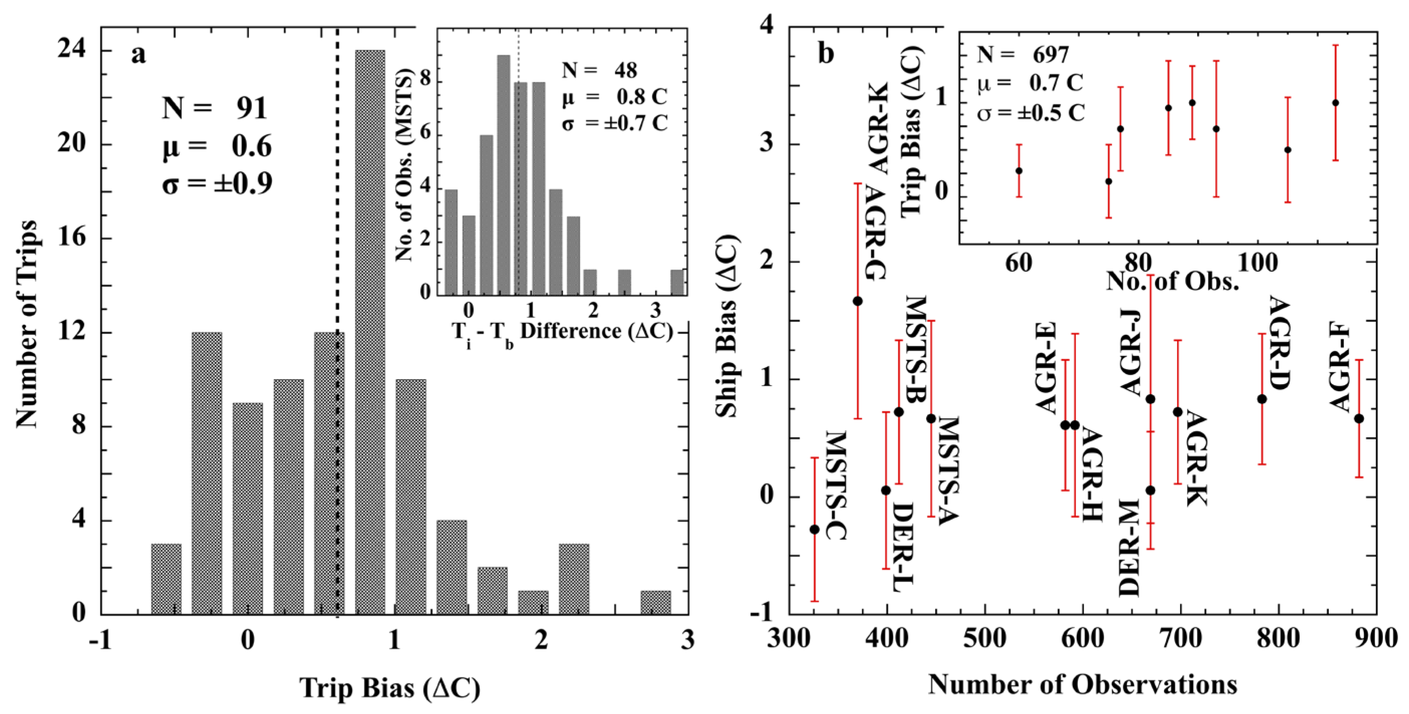
Bucket SSTs

In a unique experiment, researchers aboard the Sea Education Association (SEA) research vessel SSV Robert C. Seamans measured three sets of near-simultaneous SSTs during the S-217 transect across tropical waters, using a traditional wooden bucket (~8 L), a general-purpose ship’s canvas bucket (~11.5 L), or a meteorological rubber bucket (~0.7 L) [195]. Hourly casts using each bucket were conducted consecutively over a period of about 5 min. SSTs were measured using a traceable thermistor sensor accurate to ±0.1 °C. The three buckets yielded statistically indistinguishable SSTs, with a mean difference of 0.0 ± 0.1 °C. Given simultaneous measurements of the same waters, T_sw = T_sc = T_sr and T_mb = T_s + ε_mb, where subscript ‘s’ is sample, ‘w’, ‘c’, or ‘r’ subscripts designate wood, canvas, or rubber, respectively, ‘b’ indicates bucket, and ε_m is total measurement error. Then differencing, e.g., the wood and canvas bucket measured SSTs, (T_mw − T_mc) = (T_s + ε_mw) − (T_s + ε_mc) = (T_s − T_s) + (ε_mw − ε_mc) = Δε_mw,c. That is, differencing any two of the bucket SST measurements yields the difference of the measurement errors. If each bucket-measurement error is random and each ε_m is normally distributed, then each of the three possible Δε_m difference sets should also be normally distributed. Figure 12 shows the results of this test.

Shapiro–Wilk normality tests of the three inter-bucket error-difference data sets yielded: wood minus canvas, W(311) = 0.891, p < 0.001; rubber minus canvas, W(311) = 0.916, p < 0.001; and rubber minus wood, W(311) = 0.926, p < 0.001. Each result is consistent with non-normal inter-bucket difference errors.

The best fit to the histogram points was obtained using a Lorentzian line (Figure 12a), or a Lorentzian and Gaussian in combination (Figure 12b,c). The latter results do not necessarily indicate biphasic errors. Test fits of each $\mathsf{\Delta }{\epsilon }_{m{b}_{1,2}}$ histogram with a single Lorentzian or single Gaussian (Figure S11 of the Supplementary Materials) indicated none of them are consistent with a normal distribution. Maximally, no more than one of the three originating ε_mb sets can be random error.

Engine-Intake SSTs

The test for random error can be extended to differences between ship engine-intake and bucket SSTs. The physically correct temperature, SST_t, can vary with the sample acquisition depth [173,195,196,197]. However, surface mixing from wind and/or wave action can homogenize the thermocline [79,87,173,196,198,199]. Thus, the temperature of the engine-intake sample, T_si, and of the bucket sample, T_sb, may be similar or may differ, depending upon environmental variables. Despite the negative thermocline gradient, however, engine-intake SSTs average about 0.3 °C warmer than bucket SSTs [183,186,200].

If the thermocline is mixed into homogeneity, then T_si = T_sb, and $\Delta T_{s_{i,b}}=\Delta {\epsilon }_{m_{i,b}}$ so that the analysis under The Difference of Normal Distributions applies. To appraise the most general case, thermal non-equivalence of bucket and engine-intake seawater samples is assumed. Then T_si ≠ T_sb, T_mi = (T_si + ε_i) and T_mb = (T_sb + ε_b). Finally, T_mi − T_mb = (T_si + ε_mi) − (T_mb + ε_mb) = (T_mi − T_mb) + (ε_mi − ε_mb) = ΔT_b,I + Δε_m(b,i), where subscripts b and i refer to bucket and engine-intake samples, respectively. The differences then yield the distribution of Δε_m(b,i), but having a mean offset due to the contribution of ΔT_b,i. This condition is examined next.

• Brooks

Figure 13 shows the SST (T_i − T_b) = ΔT_b,I + Δε_m(b,i) distribution (N = 214) Charles Brooks obtained aboard the R.M.S. Empress of Britain during January–March 1924 during two West Indies cruises (9°–35° N latitude), each along nearly the same track [79].

Neither set of measurement differences nor the combined difference data set are normally distributed (Figure 13a,b, N = 214). The combined errors (Figure 13b) appear to have coalesced into a Lorentzian-like distribution similar to the land-surface temperature-measurement errors described above.

2.

WMO

During 1968–1970, the World Meteorological Organization (WMO) Working Group on Technical Problems of the Commission for Marine Meteorology carried out a program to establish the structure of (T_i − T_b) SST differences [183].

The majority of the SSTs were measured in the major ocean basins between latitudes 50° N and 50° S, but with 11% of the measurements at latitudes >50°. Routine shipboard measurement methods were employed and instruments (primarily mercury LiG thermometers) were calibrated before each voyage. Ship crew-members took measurements at standard times, using the calibrated instruments. Of a total 16,132 observer logs, 13,876 included simultaneous bucket and engine-intake SST measurements. These were acquired on at least five classes of ship under all manner of weather, wind, and cloud cover. Figure 14 is a histogram of the 13,511 T_i − T_b differences occurring within the ±3 °C range ([183]; Table 3).

The ship-board officers recruited into the WMO project likely carried out their protocols and observations with more care than common in the voluntary observing ships (VOS) program. In this event, the WMO (T_i − T_b) data set provides a reasonable estimate of a lower limit of (engine-intake)−(bucket) measurement error differences in the global record.

The (T_i − T_b) histogram in Figure 14 does not present the normal distribution expected for the differences of random measurement errors. The complex distribution was best fit with the sum of three Lorentzians (Figure S12 in the Supplementary Materials). A fit with three Gaussians was slightly poorer, but the fit serially improved with each substituted Lorentzian.

3.

Walden

Walden reported 13,847 (T_b − T_E) differences of almost simultaneous bucket (T_b) and engine-intake (T_E) SST measurements, principally carried out on German merchant ships during the early 1960s [198]. Measurement differences were categorized by latitudinal bands (0° to >55° N, S) and wind speed.

Figure 15 displays the (T_b − T_E) differences as reported by Walden for German ship SSTs measured over 25–49.9° North and South latitudes under wind speeds of 5–7 Bft and ≥8 Bft (1 Beaufort = 0.836 m/s) [198]. Global mean wind speed over the oceans is about 7.4 m/s (8.8 Bft), ranging about 1 m/s less than average in the tropics and about 1 m/s more in the 25°–75° N, S latitudes [201]. Thus, Figure 15 provides a good global estimate of typical bucket-intake SST measurement differences. Neither difference data set exhibits the normal distribution expected from random errors. The 0–1 Bft and 2–4 Bft (T_b − T_E) difference distributions reported by Walden are also non-normal.

The remaining T_{b −} T_E determinations were: 0–1 Bft, ΔT = −0.3 ± 1.2 °C and for 2–4 Bft, ΔT = −0.4 ± 1.3 °C. In every case, bucket temperatures were cooler than those recorded from engine-intake thermometers, despite the marine thermocline. Recombination of the published latitudinal (T_b − T_E) differences into a single-difference data set representing 25–49.9° N, S and all wind speeds yielded a non-normal distribution of global coverage (Figure S13 of the Supplementary Materials). Thus, regionally and globally, the T_b − T_E difference frequency histograms exhibited non-normal distributions, disconfirming the notion of random SST measurement error.

4.

Saur

Saur reported 6826 engine-intake (T_i) minus bucket (T_b) SST differences obtained during experiments conducted on 12 U.S. military ships [80]. Three were military transport ships (MSTS) sailing trans-Pacific routes between May 1959 through May 1960. Nine were radar picket ships (AGR) stationed 300 mi (186 km) off the west coast of the U.S. during September 1960–January 1962. Specialty thermometers for bucket measurements were supplied to each ship, graduated to 0.2 °F (0.1 °C), readable to 0.1 °F (0.06 °C), and were accurate to at least ±0.15 °F (0.08 °C) following calibration. The buckets were of Scripps Institute of Oceanography design, and trained personnel carried out the bucket SST measurements. The engine-intake measurements were recorded by the ship crew in routine fashion, yielding SSTs representative of typical accuracy. The intake thermometers were to ship standard, noted to have 2 °F (1.1 °C) or, occasionally, 5 °F (2.8 °C) scoring. Ship bias (μ) and standard deviation (σ) of (T_i − T_b) were calculated for each trip and each ship. Following the analysis under Difference of Normal Distributions, the assumption of random errors requires that the (T_i − T_b) differences display a normal distribution. Figure 16 shows the results of this experiment.

Figure 16a is a histogram of combined mean biases for all 6826 paired (T_i − T_b) differences acquired during 91 trips of the 12 military ships. Coalescence into a normal distribution is not in evidence. Such a coalescence is required by the assumptions of a constant distribution of random error per ship and random error means across ships. Its absence disconfirms the assumption of random measurement error. The (T_i − T_b) distribution of the single MSTS ship, (Figure 16, inset), is visually inconsistent with normality. Saur described the trip statistics as, “a typical distribution of the differences, Δ, from one trip of an MSTS ship”, indicating (T_i − T_b) differences did not produce a normal distribution for any trip of any ship.

Figure 16b displays the scatter of (T_i − T_b) means among the ships while the whiskers indicate the scatter of the trip means of each ship. Figure 16b inset shows the scatter of the (T_i − T_b) means for eight trips of radar picket ship AGR-K. The (T_i − T_b) means varied from trip to trip for a single ship. Saur’s experiment indicates that none of the 91 single trip distributions of (T_i − T_b) were normal, nor was their aggregate normally distributed.

In recognition of this state, Saur concluded that, “without improved quality control, the sea-surface temperature data reported currently and in the past are for the most part adequate only for general climatological studies …. If ship biases can be determined and corrections applied to existing sea water temperature records, it is estimated that the standard deviation of differences would be reduced to 1.3 °F (0.72 °C)”. Saur’s judgment corroborates the findings of the WMO, of Walden, and of Brooks, and is applicable to the entire SST record prior to 1963. Even were it possible to remove a mean bias (presuming the value may be determined), the 1σ = ±1.3 F (±0.72 °C) uncertainty would remain in SSTs because the non-normal (T_i − T_b) distributions indicate the random error assumption is violated and the statistical $1/\sqrt{N}$ rule is not applicable. SST errors do not average away.

Saur also discussed the accuracy experiment that Margaret K. Robinson reported and carried out aboard five U.S. Coast Guard weather ships [202]. Saur’s description of the Robinson experiment is directly relevant to the notion of SST measurement accuracy: “[T]he injection thermometers were demounted and checked at several temperatures against an accurate standard thermometer. Temperature errors from the five thermometers ranged from −2.0 °F to 1.9 °F. Results of other observations indicated that the difference between injection temperature corrected for thermometer error and surface temperature “varied erratically both among ships and on individual ships at different speeds”.”

Both Saur’s results and Robinson’s confute the assumption of random measurement error, and disconfirm the notions of constant error distributions per platform and of random error means between platforms. SST measurement error, thus, cannot be taken to reduce as $1/\sqrt{N}$.

3.4.4. T_sample and T_true

The relationship between T_s—temperature of the water sample—and T_t—the physically correct (“true”) in situ water temperature—was examined by Stevenson in an extended experiment carried out aboard the Velero IV research vessel, operated by the University of Southern California until 1985 [203]. SSTs were simultaneously measured aboard the ship and from a launch that systematically sampled nearby waters about the Velero IV. Duplicate sets of calibrated thermometers (for SST) and psychrometers (for air temperature) were used. SSTs were measured while the Velero IV was stationary or cruising, and either broadside or into the wind. The original experiment was extended to include bow-mounted thermistor probes to measure SST and air temperature while cruising. Bathythermograph (BT) casts were also carried out to evaluate bucket SSTs.

In the event, the ship was found to disturb surrounding waters under all conditions, occasionally out to 150 ft (46 m) depending upon wind conditions. Bucket SSTs measured from the Velero IV averaged about 0.5 °F (0.3 °C) cooler than the SSTs simultaneously measured from the launch. BT casts indicated bucket SSTs were consistent with the cooler water of the thermocline at 15–20 foot (4.6–6.1 m) depths. The bow-mounted probe gave reliable SSTs, but only when the Velero IV headed into the wind, or when cruising downwind at greater than wind velocity. Stevenson concluded that, “The differences in water temperatures resulting from the presence of a ship will depend, to a considerable extent, on the temperature distribution in the upper layers. The occurrence of a thoroughly mixed layer extending well below the keel depth would preclude any significant changes in temperature caused by the ship. However, should there be a shallow thermocline disturbed by the vessel’s progress, modifications of water temperatures could be extreme, or even spectacular. One may then question the value of temperatures taken aboard a ship, or from any large structure at sea. Because the measurements vary with the wind velocity and the orientation of the ship with respect to the wind direction no factor can be applied to correct the data. It is likely that the temperatures are, therefore, useless for any but gross analyses of climatic factors, excepting, perhaps, those taken with a carefully-oriented probe”.

The results indicated that a shipboard bucket seawater sample will not accurately convey the physically true sea-surface temperature unless three conditions are simultaneously true: (1) the thermocline is absent; (2) the vessel is heading into the wind; and (3) the mixing layer extends well below the depth of the keel. Thus, under nearly all conditions of the historical measurement record, T_s ≠ T_t, even when all due care was taken to protect an on-deck bucket sample from coincidental environmental impositions (primarily, wind) known to cause a temperature artefact.

That is, even when carefully executed by trained personnel, shipboard bucket SST measurements are likely to be several tenths of a Celsius offset from the physically correct SST. Although critically and centrally important, Stevenson’s experiment has received scant notice, and has not since been extended or used to qualify the global SST record. However, his conclusion confirms Saur, namely, that SSTs can contribute only to general climatological studies.

4. Discussion

This work has examined instrumental detection limits and systematic measurement errors hidden within land-surface-air and sea-surface temperatures. The impact of these measurement errors on the global air-temperature anomaly series is next discussed.

4.1. Land-Surface Air Temperatures

Air-temperature measurements contaminated with systematic error are indistinguishable from valid data. Systematically erroneous air-temperature trends will pass every statistical test used to validate a station record [7]. Harrison has noted that, “Screen–air temperature differences represent systematic errors in air temperature measurements, which, unlike random errors, are not reduced by averaging” and that “… the overall prevalence of natural ventilation effects on screen temperature measurements seems unlikely to remain constant with time [165]”.

Systematic measurement error is highly correlated among co-located naturally ventilated air-temperature sensors. This is not surprising in hindsight because the success of real-time filtering experiments has demonstrated the consistent impacts over time of radiant heating and wind speed [31,204]. Generalizing, naturally ventilated air-temperature sensors subject to similar solar heating and wind regimes will necessarily produce equivalently erroneous measurements.

Land-surface air-temperature measurements themselves are correlated across hundreds of km [19,65]. At 1200 km separation, mean correlation of anomalies is r ≈ 0.5 at latitudes > 23° and r ≈ 0.33 at latitudes < 23°. These teleconnections reflect coherently organized physical solar, wind, and precipitation phenomena within spatially extensive weather regimes [205,206,207,208,209]

Correlated weather in regional regimes ensures that widely distributed naturally ventilated land-surface air-temperature sensors will have correlated exposure to solar heating and wind effects, and, possibly, to homologous changes in local albedo. That is, multiple widely separated naturally ventilated sensors simultaneously exposed to a single overlying weather regime are effectively co-located. Though pairwise distant, they are exposed to equivalent environmental variables and, thus, to environmental impacts. On these grounds, it is proposed that systematic air-temperature-measurement error will be causally correlated across hundreds of kilometers in a manner strictly analogous to the correlation of air-temperature anomalies. Correlated systematic errors will be convolved within the correlated anomalies themselves. Cross-correlated measurement errors will be invisible within the cross-correlated anomalies.

Widely correlated systematic measurement error will not average away in a mean. Similarly, large data sets of the systematic air-temperature-measurement errors revealed in calibration experiments do not coalesce into normal distributions. There is no statistical demonstration that non-normal systematic measurement errors average away [30,210], particularly as the dimensions of error in the historical temperature record are entirely unknown.

Thus, the combination of experimental and observational grounds powerfully negates the assumption that air-temperature sensor-measurement error is exclusively random and uncorrelated. Correlated and non-normal systematic errors violate the assumptions of the central limit theorem, and disallow the statistical reduction of systematic measurement error as 1/$\sqrt{N}$. Only empirical confidence intervals from instrumental field calibrations are then available to condition measurements [211].

The proposed correlation of land-surface air-temperature sensor-measurement error across significant distances can be explicitly tested by installing calibration-competent aspirated and improved USCRN sensors adjacent to naturally ventilated USHCN sensors; most especially, those latter utilizing a LiG thermometer within a Stevenson screen [212]. The correlation of measurement errors produced by unaspirated USHCN Stevenson screens and/or MMTS shelters across arbitrary distances and topologies established by experiment can then be monitored. This experiment is recommended. Spatially correlated measurement error is expected on the above grounds.

Under these circumstances, sensor field-calibration experiments are strictly necessary to obtain the uncertainty bounds applicable to subsequent field air-temperature measurements. As noted here, few such experiments have been carried out. These, nevertheless, allow an estimate of mean systematic error in the global air-temperature record deriving from LiG thermometers in CRS and Stevenson screens and from MMTS temperature sensors.

4.2. Resolution Limits

The lower limit of resolution of LiG thermometers has been neglected during construction of the global air-temperature record. High-quality LiG thermometers scored to 1 °C or 1 °F per division have an instrumental lower limit of resolution 2σ = ±0.11 °C/°F. Qualifying this limit, Harrison noted that, “Accuracy of LiG thermometers is typically ±0.2 °C, even though their resolution may be better, for example, with 0.1 °C divisions” [93]. Fractional LiG temperatures smaller than the resolution limit have no physical meaning because they are not within the reliable detection capacity of the instrument. From Section 3.1.1, NIST calibrations of LiG thermometers and estimates of visual repeatability provide that, under ideal laboratory conditions, 2σ = ±0.33 °C/°F is the lower limit of uncertainty in any visually acquired temperature reading from a standard 1-degree/division LiG thermometer. Thus, the resolution-limited minimum uncertainty conditioning the LiG-derived air-temperature (not anomaly) record across the 20th century is, likewise, 2σ = ±0.33 °C/°F.

The non-linear thermal expansion of both mercury and ethanol, although a smaller component of measurement uncertainty, is presently uncorrected in the record. However, to the extent that structural knowledge of the LiG thermometers in use at 19th century surface stations and those used to compose earlier records is recoverable, correction for non-linearity may be possible.

Although the monthly average temperature error due to LiG nonlinearity of liquid expansion (Figure 1) will vary with the surface station and the season, its contribution to the uncertainty in global average temperature can be estimated. For this estimate, it is assumed that mercury and spirit thermometers are the sole sources of daily station maximum or minimum air temperatures, respectively, between 1900 and 1980. It is further assumed that uncertainty is distributed equally across the 0 °C ice-point calibration in a global average (Figure 1). The 1σ of uncertainty is taken to be 1/3 of the range of thermometer non-linearity. The total range shown in Figure 1 is considered to be 3σ about 0 °C. From Figure 1, the global average uncertainty due to non-linearity in a mercury-filled LiG thermometer is ±0.017 °C/°F (range ± 0.05°). For a spirit (ethanol-filled) LiG minimum thermometer the average uncertainty is ±0.33 °C/°F (range ± 1). This lower-limit estimate further assumes that 50% of all station temperatures were measured using a Fahrenheit thermometer, and that Celsius and Fahrenheit thermometers contributed equally to the global air-temperature record. The resulting estimate of global uncertainty from LiG non-linearity is shown in

Table 7. Estimate of Uncertainty in Global Averaged Temperature from LiG Non-Linearity.

Mercury	Spirit
$Va{r}_{\mathrm{C}}=0.5\times {(0.017 °C)}^2+0.5\times {(0.556\times 0.017 °F)}^2$	$Va{r}_{\mathrm{C}}=0.5\times {(0.33 °C)}^2+0.5\times {(0.556\times 0.33 °F)}^2$
$Uncertainty Variance=0.00019 °{\mathrm{C}}^2$	$Uncertainty Variance=0.0713 °{\mathrm{C}}^2$
1σnon-linearity = ±0.0138 °C	1σnon-linearity = ±0.267 °C

Var_C is the variance in Celsius-squared.

.

The complete minimal uncertainty in a global averaged land-surface air temperature through 1980 can now be derived. For the sake of the following estimate, all T_max are assumed to be from mercury LiG thermometers, while all T_min are assumed to derive from spirit LiG thermometers. From Table 7, the combined uncertainty in any daily mean land-surface air temperature due to non-linearity alone in LiG Celsius and Fahrenheit thermometers $2\sigma =1.96\times \sqrt{\left(0.00019+0.0713\right)/2}=\pm 0.371 °C$, for all T_mean = (T_min + T_max)/2.

Spirit LiG thermometers provide about half the accuracy of the mercury LiG counterpart, yielding a per-measurement 1σ = ±0.309 C/°F (cf. Section 3.1.1, Table 1). The lower limit of uncertainty in any T_min and T_max land-surface air temperature prior to 1981 consists of the detection limit and the visual repeatability (cf. Table 1) combined in quadrature with the uncertainty due to non-linearity (Table 7). For spirit LiG T_min, the merged Celsius and Fahrenheit uncertainty is,

$$2\mathsf{\sigma }\left(T_{min}^{spirit}\right)=1.96\times \sqrt{\left(0.5\times {0.309}^2\right)+0.5\times {(0.556\times 0.309)}^2+\left({0.267}^2\right)}=\pm 0.717 °\mathrm{C}.$$

(2)

and for mercury LiG T_max,

$$2\sigma \left(T_{max}^{Hg}\right)=1.96\times \sqrt{0.5\times {0.166}^2+0.5\times {(0.556\times 0.166)}^2+{0.0138}^2}=\pm 0.265$$

(3)

For T_mean = (T_max + T_min)/2, the total uncertainty in the mean is given the T_max and T_min uncertainties combined in quadrature. Thus,

$$2\sigma \left(T_{mean}\right)=1.96\times \sqrt{\left({0.366}^2+{0.135}^2\right)/2}=\pm 0.382 °\mathrm{C}$$

(4)

This ±0.382 °C represents the field-conditions lower limit of visually-read resolution-limited 2σ uncertainty to be assigned to any global daily mean land-surface meteorological LiG air temperature. During the decade after 1980, transition to MMTS sensors began [65], which is considered below.

In a monthly mean temperature $T_{mean}^M=\frac{1}{2n}{\displaystyle \sum }_{i=1}^n\left(T_i^{min}+T_i^{max}\right)$, where M is month and n is days/month. The uncertainty in T_mean for an average month (30.417 days) is the RMS of the daily means:

$$2\sigma =1.96\times \sqrt{\raisebox{1ex}{$(30.417\times [\left({0.195}^2\right)$}\!\left/ \!\raisebox{-1ex}{$30.417$}\right.}=\pm 0.382 °\mathrm{C}.$$

(5)

Likewise, for an annual land-surface air-temperature mean:

$$2\sigma =1.96\times \sqrt{\raisebox{1ex}{$12\times {(0.198)}^2$}\!\left/ \!\raisebox{-1ex}{$12$}\right.}=\pm 0.382 °\mathrm{C}.$$

(6)

Noteworthy is that the measurement uncertainty conditioning a temperature anomaly based upon the uncertainty in T_mean alone is, ($T_{mean}^M-T_{normal}^{30-year})=T_{anomaly}^M$, and $2{\sigma }_{anomaly}^M=1.96\times \pm \sqrt{{0.195}^2+{0.195}^2}=\pm 0.540 °\mathrm{C}$, where M is month.

4.3. Sea Surface

The uncertainty in a global average temperature requires a weighted combination of the lower limit uncertainties in land-surface and sea-surface temperatures. Spirit LiG thermometers make no appearance in SSTs. For the uncertainty in a mean of mercury LiG SSTs, only the 2σ = ±0.265 °C resolution and 2σ = ±0.027 °C from Hg LiG non-linearity apply. Thus, the LiG lower limit of laboratory resolution for SSTs is, $2{\sigma }_{SST}=1.96\times \sqrt{{(0.135)}^2+{(0.0138)}^2}=\pm 0.266 °\mathrm{C}.$

4.4. Global

The global land plus SST uncertainties are scaled by their respective global surface area and combined in quadrature. Thus,

$$2{\sigma }_G=1.96\times \sqrt{0.7\times {(0.136)}^2+0.3\times {(0.195)}^2}=\pm 0.306 °\mathrm{C}$$

(7)

is the lower limit of LiG uncertainty conditioning any global monthly average air temperature compiled prior to 1981.

However, global average air temperature is, typically, presented as an anomaly trend. As previously noted, in taking an anomaly, both the annual mean air temperature and the reference normal, e.g., a 1951–1980 30-year mean, will each be conditioned by the same resolution-limited ±0.308 °C. The 2σ = ±0.308 °C resolution uncertainty will, thus, separately condition both an annual mean and a 30-year normal. In calculating an annual anomaly, uncertainties in the differenced values are added in quadrature [106].

The lowest limit of uncertainty in any global annual LiG-derived air-temperature anomaly prior to 1981 is then found in the combined lower limit of detection, the non-linearity of a LiG thermometer, and the visual repeatability of measurement. The laboratory-standard resolution-limited uncertainty in a global annual air-temperature anomaly is thus

$$\pm 2{\sigma }_{Ga}=1.96\times \sqrt{{({0.156}^2)}_{AM}+{({0.156}^2)}_N}=\pm 0.432 °\mathrm{C}$$

(8)

where subscript Ga is global anomaly, AM designates annual mean temperature, and N designates the 30-year normal-period temperature mean. The statistics requiring propagation of both sources of uncertainty into differences indicate that the uncertainty of an anomaly is always greater than the uncertainty in an annual mean or in a 30-year reference normal.

Figure 17 shows the foundational 2σ = ±0.432 °C instrumental uncertainty in a temperature anomaly applied to the HadCRUT 5.0.1.0, the GISSTEMP v. 4, and the Berkeley Earth land–ocean annual temperature anomaly records [11,12,13]. The 19th century anomalies were excluded because the unknown contributions of Joule-drift render the entire early temperature trend unreliable (cf. Section 4.7). The plots terminate at 1980 because min–max temperature system (MMTS) sensors began to replace the LiG thermometer in land stations during the following decade.

Nevertheless, across the first 80 years of the 20th century, the analytically basic uncertainty following from the resolution of LiG thermometers alone yields 2σ uncertainty bounds averaging 4× the published 95% confidence interval for the global air-temperature record of 1900, more than 5× after 1950, and 13× by 1980. The uncertainty stemming from the laboratory resolution limit of LiG thermometers alone is sufficient to obscure the rate and magnitude of climate warming since 1900.

4.5. Sensor-Transfer Functions

The 1980s saw a change-over from the LiG thermometer in a louvered Stevenson/CRS shield to the new MMTS instrument featuring a thermistor in a gill shield, each of which is naturally ventilated [65,213,214]. Prior to the final change-over, several months of side-by-side CRS/MMTS comparative temperature measurements were carried out. The side-by-side measurement series allowed detection of any measurement bias offset that may distinguish the original sensor from the replacement sensor. The mean bias differentiating the measured temperatures was then removed by adjusting the mean of one temperature series into the mean of the other [65]. This offset correction is the transfer function. Difficulties applying this method to individual station series [214] are not examined here.

Generally, for an existing CRS sensor, S₁, the mean of the temperature series measured during the observational overlap time is T_m1 = T_m0 + ε_m1, where T_m0 is the unknown physically correct air-temperature mean and ε_m1 is the unknown mean-measurement error. The homologous statement for an entering MMTS sensor, S₂, is T_m2 = T_m0 + ε_m2. The transfer-function bias correction, β_1,2, to be applied is the difference between the means of the two temperature-measurement series,

$${\beta }_{1,2}=T_{m1}-T_{m2 }=\left(T_{m0}+{\epsilon }_{m1}\right)-\left(T_{m0}+{\epsilon }_{m2}\right)=\left(T_{m0}-T_{m0}\right)+\left({\epsilon }_{m1}-{\epsilon }_{m2}\right)=\Delta {\epsilon }_{m1,2}$$

(9)

where Δε_m1,2 is the difference of the unknown error means. That is, the transfer function, β_1,2, used to correct the mean S₁ → S₂ offset bias is just Δε_m1,2—the difference of the respective unknown measurement error means. The mean uncertainty in each measurement of a temperature–time series is $\pm u_T=\sqrt{\frac{{{\displaystyle \sum }}_{i=1}^n{({\epsilon }_i^t)}^2}{n}}$, where ${\epsilon }_i^t$ is the derived error in the ith measured temperature in a field-calibration experiment consisting of n measurements (cf. Section 3.3).

In applying β_1,2 to the S₂ temperature–time series, the two measurement series are no longer independent, because the Δε_m1,2 = β_1,2 mean error offset from S₁ enters into every subsequent temperature measured by S₂. Adjusting the mean of S₂ into the mean of S₁ (or vice versa) means the systematic uncertainty, ±u_T, of S₁ enters into the new S₂ series. This situation is illustrated in Figure 18, for the published CRS and MMTS adjustment series [65].

By way of explanation, the physically correct temperatures, estimated by the S₁ measurements, are unknown. The extent of knowledge is that the correct temperature mean very likely resides somewhere within the S₁ uncertainty range. Following adjustment with a transfer function, S₂ engages the uncertainty of the S₁ mean. As the entire S₂ series is offset by Δε_m1,2, the ±u_T for the S₁ mean propagates into the uncertainty of every S₂ air temperature as the root–sum–squared. The total uncertainty in each S₂ measured temperature then becomes $\pm u_2^{adj}=\sqrt{u_1^2+u_2^2}$, such that the $\pm u_2^{adj}>\pm u_2$, i.e., the transfer-function adjustment increases the uncertainty. Thus, transfer functions should cease to be used to adjust temperature series following instrumental changes in surface meteorological stations.

Similar problems will arise on making transfer-function adjustments following sensor-location moves. Field-calibration errors change with physical location because mean environmental variables shift [27], which, in turn, may produce a different ±u_T for the identical sensor [40]. Given a physical move, the sensor $\pm u_T^{ante}⋚\pm u_T^{post}$ but, in any case, if the pre- and post-move temperature series means are adjusted using a transfer function to remove a step, $\pm u_T^{ante}$ must propagate into the subsequently measured air temperatures.

4.6. A Lower Limit of Uncertainty in the Global Averaged Surface Air Temperature to 2010

The uncertainties due to resolution and to systematic measurement error are now combined to produce a global average anomaly trend conditioned with metrologically valid lower-limit uncertainty bounds. For the years 1900–1980, the instrumental resolution uncertainties in land-surface global air temperatures 2σ = ±0.382 °C and SSTs 2σ = ±0.266 °C, are brought down from Section 4.2 and Section 4.3.

To these must be added the uncertainty stemming from the non-random systematic measurement error revealed by the calibration experiments of land-surface air-temperature sensors. The several CRS and MMTS calibrations from Table 6 are assumed to have equivalent statistical validity and to adequately sample the impacts of varying physical environments. The unweighted mean of known LiG/CRS systematic calibration error is 2σ = ±0.58 °C. Following 1990, the lower-limit calculation allows MMTS sensors to have replaced LiG/CRS sensors worldwide. The mean of MMTS calibration uncertainty 2σ = ±0.56 °C is, therefore, applied under the same assumptions. Following 2005, the uncertainty in MMTS in land-surface temperatures is replaced by the 2σ = ±0.1 °C resolution and 2σ = ±0.47 °C electronic uncertainty (over −20 °C to 30 °C) in the Climate Research Network (CRN) sensor [212,215].

For SSTs, the available bucket and engine-intake field calibrations show that shipboard SST measurement errors are, likewise, not random. The uncertainties attached to bucket SSTs, 2σ = ±0.4 °C and engine-intake SSTs 2σ = ±2 °C are taken from the calibration experiments reported by Tabata carried out aboard the C.F.A.V. Endeavor oceanographic vessel [81]. The calibration-error difference, ε_EI − ε_B = ±0.8 °C, is well within the set of reported mean-measurement differences described above.

A small but significant fraction of SSTs falls under unknown methods of measurement [176]. For these, the lower-limit calculation required assignment of the bucket uncertainty prior to 1931, followed by zero from 1932 to 1945. After 1946, uncertainty of unknown methods was calculated as the RMS of 0.33 bucket, 0.33 engine-intake, and 0.33 bathythermograph (BT) measurements (2σ_bathy = ±0.3 °C) [216]. The resulting systematic SST uncertainty 2σ = ±0.62 °C is dominated by engine-intake uncertainty. One calibration of surface drifters showed only random temperature errors [217]. However, buoy temperature-measurement errors may not be random everywhere [86,89].

Fractions of SSTs entering the record from bucket, engine-intake, and unknown methods were derived from published data [176]. All final uncertainties in air temperature are root–sum–squares of entering calibration errors or uncertainties. The uncertainty in global annual temperature from a land-surface LiG thermometer is,

$$\pm u_{LS}=\sqrt{u_{res}^2+u_{acc}^2+u_{nonlin}^2+u_{sys}^2},$$

(10)

where subscript res is visual resolution, acc is accuracy, nonlin is non-linearity of response, and sys is the mean systematic measurement error induced by environmental variables. For MMTS sensors, there was no term for visual resolution or non-linearity. The uncertainty in each annual LiG SST is,

$$\pm u_{SST}=\sqrt{{(f_b\times {\epsilon }_b)}^2+{(f_{EI}\times {\epsilon }_{EI})}^2+{(f_{unk}\times {\epsilon }_{unk})}^2},$$

(11)

where f is fraction of SSTs by that method, as provided in published work [176]. Subscript ε is error of the method, b is bucket, EI is engine-intake, and unk is unknown method. The sum of fractions, f_b + f_EI + f_unk = 1. The fractional contribution of each method to SST and their derivation are provided in the tab-delimited text file, “Calculation of SST Fractions” in the Supplementary Materials. The final annual uncertainty in global air temperature was calculated as,

$$\pm u_G=\sqrt{0.3\times u_{LST}^2+0.7\times u_{SST}^2},$$

(12)

where subscript LST is land-surface air temperature and SST is sea-surface temperature.

Table 8. Lower Limit of Uncertainty (±2σ) Entering the Global Air-Temperature Record.

Land Surface		Sea Surface
Instrumental		Instrumental (LiG; 1 °C/division) a
accuracy (LiG; 1 °C/division) a	0.30	accuracy	0.30
visual repeatability (LiG; 1 °C/division) a	0.144	visual repeatability	0.144
non-linearity (LiG; 1 °C/division) a	0.371	non-linearity	0.017
MMTS b	0.196
Systematic		Systematic
Stevenson/CRS b	0.58	bucket	0.30 d
MMTS b	0.56	engine-intake	2.0 d
Instrumental (USCRN) c		bathythermograph	0.30 e
sensor resolution	0.10
self-heating f	0.48

^aTable 1. ^b Table 6. ^c ref. [212]. ^d ref. [81]. ^e ref. [216]. ^f ref. [212].

provides the separate uncertainties entering the global record.

As before, in calculating the uncertainty in an anomaly, the uncertainty in air temperature must be combined in quadrature with the uncertainty in a 30-year normal (

Table 9. 30-Year Normal Periods, Anomalies, Trends, and Uncertainties.

Normal Period	Anomaly Mean (Δ°C) a	RMS 2σ Uncertainty (±°C)	100-Year Trend (Δ°C) a
1901–1930	−0.30	0.71	0.79
1911–1940	−0.20	0.73	1.23
1921–1950	−0.09	1.15	0.74
1931–1960	−0.03	1.41	0.26
1941–1970	−0.91	1.57	−0.31
1951–1980	0.0	1.48	0.40
1961–1990	0.09	1.49	1.50
1971–2000	0.24	1.44	1.82
1981–2010	0.43	1.26	0.0

^a Relative to a 1951–1980 normal.

). The globally averaged surface air-temperature-anomaly record amended with the ±2σ (95%) lower limit of uncertainty resulting from these calculations is shown in Figure 19. In constructing Figure 19, the 1951–1980 NASA/GISS 30-year normal was chosen [19], with RMS uncertainty 1σ = ±0.758 °C (cf. Table 9). The details of the calculation may be found in the tab-delimited ASCII-column text files in the Supplementary Materials. The uncertainty bounds represent a lower limit, including:

• The accuracy—the limit of detection of high-quality 1 °C/division mercury LiG thermometers;
• The resolution—the limit of visual repeatability of a temperature reading under ideal laboratory conditions;
• The non-linearity of LiG response to temperature;
• The land-station systematic field-measurement uncertainty from calibrations of well-sited and well-maintained sensors;
• The SST bucket, engine-intake, and bathythermograph uncertainties from calibrations by trained personnel aboard an ocean research vessel.

The majority of uncertainty after 1945 derives from inclusion of engine-intake measurements with their calibration uncertainty. Over 1981–1989, CRS error was transitioned to MMTS error by linear interpolation. LiG resolution was not included after 1989, while only MMTS errors were included for land-surface error from 1990–2004. After 2005 for land-surface air temperatures, only the measurement uncertainty of the Climate Research Network sensor was included. SST uncertainties included LiG resolution and calibration uncertainty. Random errors from drifting and moored buoys were not included in the total uncertainty. Anomalies prior to 1900 were excluded because Joule-drift renders the early record unreliable through 1890 at least. Uncertainty increases after 1945 because engine-intake SSTs come to dominate the record in the second half of the 20th century. Table 9 summarizes the temperature anomaly statistics for the nine 30-year normal periods between 1901 and 2010.From Figure 19, the mean global air-temperature-record anomaly over the 20th century (1900–1999) is 0.74 ± 1.94 °C. The 2σ = ±1.94 °C uncertainty does not indicate a range of possible temperatures but, rather, the range of ignorance over which no information is available [219,220,221]. That is, the physically correct mean anomaly may be anywhere within that range. Relative to the 1951–1980 normal, the anomaly mean ± 2σ RMS uncertainty for 1900–1945 is −0.21 ± 1.7 °C, for 1946–1980, −0.01 ± 2.1 °C, for 1981–2004, 0.37 ± 2.0 °C, and for 2005–2010, 0.66 ± 1.6 °C. Changing the normal period to the originally proposed 1901–1930 normal [1,222], reduces the anomaly uncertainty by about 1/3. Reporting the air-temperature trend rather than the anomaly trend would reduce the mean uncertainty by about two-fold (1951–1980 normal).

4.7. Joule-Drift

Joule-drift is discussed here because it does not enter into appraisals of the 20th century anomaly record. However, the Joule-drift of lead-glass or soft-glass thermometers fatally compromises temperature measurements prior to 1890. On the continuous use of such thermometers, Joule-drift would have added a spurious warming trend of about 0.6–0.7 °C/°F per century to a surface-station temperature record through the 19th century. This problem was well-known to contemporaneous meteorologists. Thus, “In considering the well-worn question of the zero-movements of thermometers, … for example [regarding] the thermometer … verified at Kew Observatory … I knew that the zero would probably rise and that the amount of the rise would not be the same in my case as in that of others and that therefore, I must obtain the index-error experimentally” [129]. Similarly, “The upward displacement of the zero in mercury thermometers used in the Specola in the second half of the 19th century was about 0.3–0.6 °C, as demonstrated by the accurate measurements carried out in the second half of the 19th century, noted in the observation registers” [112]. Specola Astronomic Observatory is now the Astronomical Observatory of Padua. However, the previously well-understood lesson of Joule-drift has evidently been latterly forgotten.

Recovery of early historical air-temperature series is an on-going major project [223,224,225,226,227]. However, quality-assurance methodologies for early temperature series do not mention instrumental detection limits or correction for LiG non-linearity, and stand silent on the impact of Joule-drift [223,225,228,229]. Individual reports of recovery of early historical land-surface air-temperature series, likewise, do not mention the problems of LiG thermometer non-linearity or of Joule-drift [230,231,232,233,234,235,236,237,238,239,240,241,242], with exceptions as notable as they are rare [112,113,115,243,244,245,246]. The unknown but inevitable impact of systematic measurement errors that accrue to naturally ventilated sensors is, likewise, by-passed in silence. Incorporation of these uncorrected and unreliable early historical air-temperature series into modern compilations will necessarily produce spurious trends and unfounded conclusions.

The X-ray-emission analysis reported here demonstrates that some meteorological thermometers continued to be constructed of lead-glass until at least 1900. No recognition of Joule-drift, detection limits, or non-linearity of response appears in the modern compilations of meteorological station air temperatures [83,247,248]. Likewise, temperature corrections for Joule-drift or nonlinearity are not mentioned in the mid-20th century initializing reports of hemispheric or global average air temperatures, where the fundamentals of methodology should appear [3,19,51,52,53,83,249,250]. Nor are they found at the contemporary GISSTEMP explanatory website [251], nor the reported Berkeley Earth global temperature record [252].

Undetected Joule-drift in the 19th century global air-temperature record renders uncertain any warming trend prior to 1900. Correction for the likely impact of Joule-drift prior to 1900 appears impossible.

5. Conclusions

This work has presented an analysis that is some 40 years overdue, namely, critical application of metrological standards of instrumental resolution, calibration, measurement error, and uncertainty [253,254,255], to meteorological air-temperature instruments and measurements.

5.1. Major Findings

With respect to the published global air-temperature record, the major findings are:

• The accuracy limit of LiG meteorological thermometers, 2σ = ±0.11 °C/°F, had been ignored;
• The laboratory lower-limit ideal of visual repeatability of LiG thermometer, 2σ = ±0.144 °C/°F, had been ignored;
• The published uncertainty of the 1900–1980 global average air-temperature anomaly record was less than the combined 2σ = ±0.432 °C laboratory ideal lower limit of resolution of high-quality LiG thermometers;
• Joule-drift of pre-1890 lead-glass or soft-glass thermometers had been ignored, but renders unreliable the early air-temperature record through the 19th century;
• Lead-glass meteorological thermometers were still manufactured and entering use in 1900;
• Land- and sea-surface temperatures had not been corrected for the non-linear response of LiG thermometers;
• Systematic measurement error produced by naturally ventilated land-surface air-temperature sensors is not random;
• Systematic land-surface air-temperature-measurement error is correlated across sensors;
• The semivariogram method does not reveal mean SST measurement error, but rather, half the mean difference in error, i.e., 0.5Δε_µ;
• The mean error in SST measurements remains unknown (as does the marine wind measurement error mean);
• Bucket SST measurement error is typically not random;
• Engine-intake SST measurement error is not random;
• The distribution of ship SST measurement error varies with each trip, with the crew (and even with the watch), and between ships;
• Means of ship SST error distributions are themselves not randomly distributed;
• Turbulence caused by the ship (platform) itself generally obviates the correspondence of the measurement to the undisturbed state of surface waters. In-situ SST measurements that may be accurate, will nevertheless be physically incorrect.

LiG thermometer Joule-drift has rendered the entire early air-temperature record through the 19th century unreliable. Field-calibration experiments of air temperature and ship SST sensors uniformly disconfirm the assumption that air temperature and SST measurement error is strictly random. Exceptions may include bucket SST measurements carried out by methodologically trained personnel and SSTs measured using modern buoys.

The compilation of land- and sea-surface LiG uncertainty yield a 1900–2010 global air-temperature record anomaly of 0.86 ± 1.92 °C (2σ), which renders impossible any conclusion regarding the rate or magnitude of climate warming since 1850 or earlier.

5.2. Involve the ASPE

Before any further policy decisions are to be made on the grounds of a warming climate, full and complete analysis of the air and sea-surface temperature record must be engaged, completed, and reported by multiple independent professionally disinterested and metrologically expert third-party engineering groups. Only this will resolve the forefront problem of reliability brought into focus here. Notions of unprecedented warming and disastrous outcomes deriving from the previously published air-temperature record are scientifically unsustainable. Their wider significance must, instead, await unconflicted metrological and economic analyses. Causality remains deeply at issue [256,257,258,259,260,261].

A first order of business might be to fully evaluate the systematic field-measurement errors of surface air-temperature meteorological field stations. Climate Research Network aspirated sensors, modified to produce more highly accurate measurements [212], might be placed near selected CRS and MMTS field-station sensors of the Global Historical Climatology Network. Automation to retrieve LiG thermometer readings is available [262,263]. The systematic measurement errors made by CRS/LiG and MMTS sensors in working meteorological field-stations could then be evaluated under a complete sampling of the impacts of environmental circumstance. A full inventory of poorly-sited surface stations should be included in the experiment so as to ensure a comprehensive survey [264,265,266,267,268,269].

These calibration experiments would provide the first thorough evaluation of the reliability of land-surface field station air-temperature measurements. The integrity of individual, regional, and, ultimately, global land-surface air temperatures would become available. The calibration uncertainties derived would be applicable to a historically valid estimate of uncertainty in the annually resolved global average land-surface air-temperature record dating back to 1900. The presence and magnitudes of inter-sensor cross-correlations across increasing distances could then also be determined. The described calibration experiment would be expensive. However, the cost is trivial compared to the ~39 billion USD spent on scientific and technical research between 1990–2018 [270], to ameliorate a problem now known to be objectively invisible (this work, and [256,257,258,271,272]).

The global averaged surface air-temperature record has been central to notions of unprecedented and dangerous climate warming for at least 35 years [19,20,21]. The 1990 Summary for Policymakers of the First Assessment Report (1AR) produced by the Intergovernmental Panel on Climate Change (IPCC) warned of, “a rate of increase of global mean temperature during the next century of about 0.3 °C per decade …, this is greater than that seen over the past 10,000 years [22]”. Likewise, the 2021 IPCC 6AR Summary for Policymakers begins, “It is unequivocal that human influence has warmed the atmosphere, ocean and land [24]”. However, this and prior work show that neither statement can be sustained on scientific grounds [7,69,256,257,258,259,260,261,271].

Given the scope of the warnings and the enormous expenditures and economic dislocations in the name of climate warming [273], it is not an exaggeration to suppose that a comprehensive societal effort would have been expended to ensure the scientific basis validating a cause for worry. However, a comprehensive competent third-party metrological evaluation of the historical air-temperature record by precision engineers is notably absent. At the same time, the present work has shown that production of the record has sorely lacked the necessary attention to detail. Critical assumptions remained untested, and analyses wanted the deep care demanded by scientific rigor. The first order of business in experiment is to evaluate the reliability of the instrument, followed by assessing the quality of the data. Remarkably, the current global air-temperature record evidences no understanding of LiG thermometers, of their history, or of their metrology.

Very evidently, a professionally competent and disinterested third party must be commissioned to produce a full and rigorous instrumental engineering evaluation of the historical temperature record. It is here recommended that the American Society for Precision Engineering constitutes one such independent and competent third party. Along with precision engineering societies from other countries, their full, independently replicated, and delivered evaluations of meteorological air temperatures must precede any further actions.

5.3. Final Conclusions

Direct evidence of a warming climate since the 19th century includes the lengthened growing season, the revegetation of the far North, and the poleward migration of the northern tree line [274,275,276,277,278,279,280,281,282,283]. However, at the 95% level of uncertainty, neither the rate nor the magnitude of 19th or 20th century warming can be known. A more detailed appraisal of errors may modify the uncertainty bounds, but an alternative conclusion is unlikely.

The 20th century surface air-temperature anomaly, 0.74 ± 1.94 °C (2σ), does not convey any knowledge of rate or magnitude of change in the thermal state of the troposphere. Climate alarm on that account is unjustifiable. The Joule-drift that certainly plagued all LiG thermometers manufactured prior to 1885 obviates the reliability of earlier air-temperature measurements. The global averaged surface air-temperature anomaly record cannot sustain any notion of unprecedented climate warming over the last 200 years, or over any other timespan.

References

- Ahlmann, H.W. The Present Climatic Fluctuation. Geogr. J. 1948, 112, 165–193. [Google Scholar] [CrossRef]
- Willett, H.C. Patterns of world weather changes. Eos Trans. Am. Geophys. Union 1948, 29, 803–809. [Google Scholar] [CrossRef]
- Mitchell, J.M., Jr. Recent Secular Changes of Global Temperature. Ann. N. Y. Acad. Sci. 1961, 95, 235–250. [Google Scholar] [CrossRef]
- Mitchell, J.M. On the Causes of Instrumentally Observed Secular Temperature Trends. J. Atmos. Sci. 1953, 10, 244–261. [Google Scholar] [CrossRef]
- Hubbard, K.G.; Lin, X.; Walter-Shea, E.A. The Effectiveness of the ASOS, MMTS, Gill, and CRS Air Temperature Radiation Shields. J. Atmos. Ocean. Technol. 2001, 18, 851–864. [Google Scholar] [CrossRef]
- Georges, C.; Kaser, G. Ventilated and unventilated air temperature measurements for glacier-climate studies on a tropical high mountain site. J. Geophys. Res. Atmos. 2002, 107, ACL 15-1–ACL 15-10. [Google Scholar] [CrossRef]
- Frank, P. Systematic Error in Climate Measurements: The global air temperature record. In Proceedings of the Role of Science in the Third Millennium, Singapore, 19–25 August 2016; pp. 337–351. [Google Scholar]
- Sparks, W.R. The Effect of Thermometer Screen Design on the Observed Temperature; Davis, D.A., Ed.; World Meteorological Organization: Geneva, Switzerland, 1972.
- Naylor, S. Thermometer screens and the geographies of uniformity in nineteenth-century meteorology. Notes Rec. R. Soc. J. Hist. Sci. 2019, 73, 203–221. [Google Scholar] [CrossRef]
- Jones, P. The reliability of global and hemispheric surface temperature records. Adv. Atmos. Sci. 2016, 33, 269–282. [Google Scholar] [CrossRef]
- Lenssen, N.J.L.; Schmidt, G.A.; Hansen, J.E.; Menne, M.J.; Persin, A.; Ruedy, R.; Zyss, D. Improvements in the GISTEMP Uncertainty Model. J. Geophys. Res. Atmos. 2019, 124, 6307–6326. [Google Scholar] [CrossRef]
- Morice, C.P.; Kennedy, J.J.; Rayner, N.A.; Winn, J.P.; Hogan, E.; Killick, R.E.; Dunn, R.J.H.; Osborn, T.J.; Jones, P.D.; Simpson, I.R. An Updated Assessment of Near-Surface Temperature Change From 1850: The HadCRUT5 Data Set. J. Geophys. Res. Atmos. 2021, 126, e2019JD032361. [Google Scholar] [CrossRef]
- Rohde, R.A.; Hausfather, Z. The Berkeley Earth Land/Ocean Temperature Record. Earth Syst. Sci. Data 2020, 12, 3469–3479. [Google Scholar] [CrossRef]
- Shackleton, N.J. Attainment of isotopic equilibrium between ocean water and the benthonic foraminifera genus Uvigerina: Isotopic changes in the ocean during the last glacial. In Proceedings of the Colloques Internationaux du Centre National de la Recherche Scientifique, Gif-Sur-Yvette, France, 5–9 June 1973; Volume 219, pp. 203–209. [Google Scholar]
- Schneider, S.H. On the Carbon Dioxide-Climate Confusion. J. Atmos. Sci. 1975, 32, 2060–2066. [Google Scholar] [CrossRef]
- Mitchell, J.M., Jr. Carbon Dioxide and Future Climate. EDS Environ. Data Serv. March 1977, 3–9. [Google Scholar] [CrossRef]
- Miles, M.K. Predicting temperature trend in the Northern Hemisphere to the year 2000. Nature 1978, 276, 356–359. [Google Scholar] [CrossRef]
- Charney, J.G.; Arakawa, A.; Baker, D.J.; Bolin, B.; Dickinson, R.E.; Goody, R.M.; Leith, C.E.; Stommel, H.M.; Wunsch, C.I. Carbon Dioxide and Climate: A Scientific Assessment; National Academy of Sciences: Washington, DC, USA, 1979; p. 18. [Google Scholar]
- Hansen, J.; Lebedeff, S. Global Trends of Measured Surface Air Temperature. J. Geophys. Res. 1987, 92, 13345–13372. [Google Scholar] [CrossRef]
- Hansen, J. Statement of Dr. James Hansen, Director, NASA Goddard Institute for Space Studies. Available online: http://image.guardian.co.uk/sys-files/Environment/documents/2008/06/23/ClimateChangeHearing1988.pdf (accessed on 4 June 2021).
- Hansen, J.; Fung, I.; Lacis, A.; Rind, D.; Lebedeff, S.; Ruedy, R.; Russell, G.; Stone, P. Global Climate Changes as Forecast by Goddard Institute for Space Studies Three-Dimensional Model. J. Geophys. Res. 1988, 93, 9341–9364. [Google Scholar] [CrossRef]
- IPCC. Climate Change: The IPCC Scientific Assessment. In Contribution of Working Group I to the First Assessment Report of the Intergovernmental Panel on Climate Change; Houghton, J.T., Jenkins, G.J., Ephraums, J.J., Eds.; Cambridge University: Cambridge, UK, 1990; p. 365. [Google Scholar]
- Hansen, J.; Wilson, H. Commentary on the significance of global temperature records. Clim. Chang. 1993, 25, 185–191. [Google Scholar] [CrossRef]
- IPCC. Summary for Policymakers. In Climate Change 2021: The Physical Science Basis—Contribution of Working Group I to the Sixth Assessment Report of the Intergovernmental Panel on Climate Change; Masson-Delmotte, V., Zhai, P., Pirani, A., Connors, S.L., Péan, C., Berger, S., Caud, N., Chen, Y., Goldfarb, L., Gomis, M.I., et al., Eds.; Cambridge University Press: Cambridge, UK; New York, NY, USA, 2021; pp. 3–32. [Google Scholar]
- Alexander, M.D.; MacQuarrie, K.T.B. Toward a Standard Thermistor Calibration Method: Data Correction Spreadsheets. Groundw. Monit. Remediat. 2005, 25, 75–81. [Google Scholar] [CrossRef]
- Stillman, R. Downstream from calibration. In Proceedings of the IEE Colloquium on Contribution of Instrument Calibration to Product Quality—Part 2, London, UK, 25 April 1995; pp. 9/1–9/2. [Google Scholar]
- Barcelo-Ordinas, J.M.; Doudou, M.; Garcia-Vidal, J.; Badache, N. Self-calibration methods for uncontrolled environments in sensor networks: A reference survey. Ad Hoc Netw. 2019, 88, 142–159. [Google Scholar] [CrossRef]
- Tellinghuisen, J. Calibration: Detection, Quantification, and Confidence Limits Are (Almost) Exact When the Data Variance Function Is Known. Anal. Chem. 2019, 91, 8715–8722. [Google Scholar] [CrossRef]
- Abernethy, R.B.; Benedict, R.P.; Dowdell, R.B. ASME Measurement Uncertainty. J. Fluids Eng. 1985, 107, 161–164. [Google Scholar] [CrossRef]
- Vasquez, V.R.; Whiting, W.B. Accounting for Both Random Errors and Systematic Errors in Uncertainty Propagation Analysis of Computer Models Involving Experimental Measurements with Monte Carlo Methods. Risk Anal. 2006, 25, 1669–1681. [Google Scholar] [CrossRef] [PubMed]
- Hubbard, K.G.; Lin, X. Realtime data filtering models for air temperature measurements. Geophys. Res. Lett. 2002, 29, 67-1–67-4. [Google Scholar] [CrossRef]
- Lin, X.; Hubbard, K.G.; Baker, C.B. Surface Air Temperature Records Biased by Snow-Covered Surface. Int. J. Climatol. 2005, 25, 1223–1236. [Google Scholar] [CrossRef]
- MacHattie, L.B. Radiation Screens for Air Temperature Measurement. Ecology 1965, 46, 533–538. [Google Scholar] [CrossRef]
- Huband, N.D.S.; King, S.C.; Huxley, M.W.; Butler, D.R. The performance of a thermometer screen on an automatic weather station. Agric. For. Meteorol. 1984, 33, 249–258. [Google Scholar] [CrossRef]
- Erell, E.; Leal, V.T.; Maldonado, E. Measurement of air temperature in the presence of a large radiant flux: An assessment of passively ventilated thermometer screens. Bound.-Layer Meteorol. 2005, 114, 205–231. [Google Scholar] [CrossRef]
- Huwald, H.; Higgins, C.W.; Boldi, M.-O.; Bou-Zeid, E.; Lehning, M.; Parlange, M.B. Albedo effect on radiative errors in air temperature measurements. Water Resour. Res. 2009, 45, W08431. [Google Scholar] [CrossRef]
- Yang, J.; Deng, X.; Liu, Q.; Ding, R. Temperature error-correction method for surface air temperature data. Meteorol. Appl. 2020, 27, e1972. [Google Scholar] [CrossRef]
- Yang, J.; Liu, Q.; Dai, W. A method for solar radiation error correction of temperature measured in a reinforced plastic screen for climatic data collection. Int. J. Climatol. 2018, 38, 1328–1336. [Google Scholar] [CrossRef]
- Harrison, R.G. Lag-time effects on a naturally ventilated large thermometer screen. Q. J. R. Meteorol. Soc. 2011, 137, 402–408. [Google Scholar] [CrossRef]
- Yamamoto, K.; Togami, T.; Yamaguchi, N.; Ninomiya, S. Machine Learning-Based Calibration of Low-Cost Air Temperature Sensors Using Environmental Data. Sensors 2017, 17, 1290. [Google Scholar] [CrossRef]
- Wendland, W.M.; Armstrong, W. Comparison of Maximum-Minimum Resistance and Liquid-in-Glass Thermometer Records. J. Atmos. Ocean. Technol. 1993, 10, 233–237. [Google Scholar] [CrossRef]
- Lin, X.; Hubbard, K.G.; Walter-Shea, E.A.; Brandle, J.R.; Meyer, G.E. Some Perspectives on Recent In Situ Air Temperature Observations: Modeling the Microclimate inside the Radiation Shields*. J. Atmos. Ocean. Technol. 2001, 18, 1470–1484. [Google Scholar] [CrossRef]
- Young, F.D. Influence of exposure on temperature observations. Mon. Weather Rev. 1920, 48, 709–711. [Google Scholar] [CrossRef]
- Aitken, J. 4. Thermometer Screens. Proc. R. Soc. Edinb. 1884, 12, 661–696. [Google Scholar] [CrossRef]
- Harrison, R.G.; Burt, S.D. Quantifying uncertainties in climate data: Measurement limitations of naturally ventilated thermometer screens. Environ. Res. Commun. 2021, 3, 061005. [Google Scholar] [CrossRef]
- Attivissimo, F.; Cataldo, A.; Fabbiano, L.; Giaquinto, N. Systematic errors and measurement uncertainty: An experimental approach. Measurement 2011, 44, 1781–1789. [Google Scholar] [CrossRef]
- Vasquez, V.R.; Whiting, W.B. Uncertainty of predicted process performance due to variations in thermodynamics model parameter estimation from different experimental data sets. Fluid Phase Equilib. 1998, 142, 115–130. [Google Scholar] [CrossRef]
- Taylor, B.N.; Kuyatt, C.E. Guidelines for Evaluating and Expressing the Uncertainty of NIST Measurement Results; National Institute of Standards and Technology: Washington, DC, USA, 1994; p. 20.
- Damon, P.E.; Kunen, S.M. Global Cooling? Science 1976, 193, 447–453. [Google Scholar] [CrossRef]
- Kukla, G.J.; Angell, J.K.; Korshover, J.; Dronia, H.; Hoshiai, M.; Namias, J.; Rodewald, M.; Yamamoto, R.; Iwashima, T. New data on climatic trends. Nature 1977, 270, 573–580. [Google Scholar] [CrossRef]
- Hansen, J.; Johnson, D.; Lacis, A.; Lebedeff, S.P.L.; Rind, D.; Russell, G. Climate Impact of Increasing Atmospheric Carbon Dioxide. Science 1981, 213, 957–966. [Google Scholar] [CrossRef]
- Jones, P.D.; Wigley, T.M.L.; Kelly, P.M. Variations in Surface Air Temperatures: Part 1. Northern Hemisphere, 1881–1980. Mon. Weather Rev. 1982, 110, 59–70. [Google Scholar] [CrossRef]
- Jones, P.D.; Raper, S.C.B.; Bradley, R.S.; Diaz, H.F.; Kellyo, P.M.; Wigley, T.M.L. Northern Hemisphere Surface Air Temperature Variations: 1851–1984. J. Clim. Appl. Meteorol. 1986, 25, 161–179. [Google Scholar] [CrossRef]
- Menne, M.J.; Durre, I.; Vose, R.S.; Gleason, B.E.; Houston, T.G. An Overview of the Global Historical Climatology Network-Daily Database. J. Atmos. Ocean. Technol. 2012, 29, 897–910. [Google Scholar] [CrossRef]
- Hansen, J.; Ruedy, R.; Sato, M.; Lo, K. Global Surface Temperature Change. Rev. Geophys. 2010, 48, RG4004. [Google Scholar] [CrossRef]
- Karl, T.R. Perspective on Climate Change in North America During the Twentieth Century. Phys. Geogr. 1985, 6, 207–229. [Google Scholar] [CrossRef]
- Yamamoto, R.; Iwashima, T.; Hoshiai, M. Change of the Surface Air Temperature Averaged over the Northern Hemisphere and Large Volcanic Eruptions during the Year 1951–1972. J. Meteorol. Soc. Japan. Ser. II 1975, 53, 482–486. [Google Scholar] [CrossRef]
- Starr, V.P.; Oort, A.H. Five-Year Climatic Trend for the Northern Hemisphere. Nature 1973, 242, 310–313. [Google Scholar] [CrossRef]
- Brohan, P.; Kennedy, J.J.; Harris, I.; Tett, S.F.B.; Jones, P.D. Uncertainty estimates in regional and global observed temperature changes: A new data set from 1850. J. Geophys. Res. 2006, 111, D12106. [Google Scholar] [CrossRef]
- Mobley, C.D.; Preisendorfer, R.W. Statistical Analysis of Historical Climate Data Sets. J. Appl. Meteorol. 1985, 24, 555–567. [Google Scholar] [CrossRef]
- Callendar, G.S. Temperature fluctuations and trends over the earth. Q. J. R. Meteorol. Soc. 1961, 87, 1–12. [Google Scholar] [CrossRef]
- Yamamoto, R.; Hoshiai, M. Recent Change of the Northern Hemisphere Mean Surface Air Temperature Estimated by Optimum Interpolation. Mon. Weather Rev. 1979, 107, 1239–1244. [Google Scholar] [CrossRef]
- Hansen, J.; Ruedy, R.; Glascoe, J.; Sato, M.M. GISS analysis of surface temperature change. J. Geophys. Res. 1999, 104, 30997–31022. [Google Scholar] [CrossRef]
- Muller, R.A.; Wurtele, J.; Rohde, R.; Jacobsen, R.; Perlmutter, S.; Rosenfeld, A.; Curry, J.; Groom, D.; Wickham, C.; Mosher, S. Earth Atmospheric Land Surface Temperature and Station Quality in the Contiguous United States. Geoinform. Geostat. Overv. 2013, 1, 2. [Google Scholar] [CrossRef]
- Quayle, R.G.; Easterling, D.R.; Karl, T.R.; Hughes, P.Y. Effects of Recent Thermometer Changes in the Cooperative Station Network. Bull. Amer. Met. Soc. 1991, 72, 1718–1723. [Google Scholar] [CrossRef]
- Frank, P. Uncertainty in the Global Average Surface Air Temperature Index: A Representative Lower Limit. Energy Environ. 2010, 21, 969–989. [Google Scholar] [CrossRef]
- Anderson, S.P.; Baumgartner, M.F. Radiative Heating Errors in Naturally Ventilated Air Temperature Measurements Made from Buoys. J. Atmos. Ocean. Technol. 1998, 15, 157–173. [Google Scholar] [CrossRef]
- Andersson, T.; Mattisson, I. A Field Test of Thermometer Screens, SMHI RMK No. 62; RMK 62; Swedish Meteorological and Hydrology Institute: Norrköping, Sweden, 1991; p. 41. [Google Scholar]
- Frank, P. Negligence, Non-Science, and Consensus Climatology. Energy Environ. 2015, 26, 391–416. [Google Scholar] [CrossRef]
- Atkinson, C.P.; Rayner, N.A.; Roberts-Jones, J.; Smith, R.O. Assessing the quality of sea surface temperature observations from drifting buoys and ships on a platform-by-platform basis. J. Geophys. Res. Ocean. 2013, 118, 3507–3529. [Google Scholar] [CrossRef]
- Kent, E.C.; Berry, D.I. Quantifying random measurement errors in Voluntary Observing Ships’ meteorological observations. Int. J. Climatol. 2005, 25, 843–856. [Google Scholar] [CrossRef]
- Rayner, N.A.; Brohan, P.; Parker, D.E.; Folland, C.K.; Kennedy, J.J.; Vanicek, M.; Ansell, T.J.; Tett, S.F.B. Improved Analyses of Changes and Uncertainties in Sea Surface Temperature Measured In Situ since the Mid-Nineteenth Century: The HadSST2 Dataset. J. Clim. 2006, 19, 446–469. [Google Scholar] [CrossRef]
- Kennedy, J.J.; Rayner, N.A.; Smith, R.O.; Parker, D.E.; Saunby, M. Reassessing biases and other uncertainties in sea surface temperature observations measured in situ since 1850: 1. Measurement and sampling uncertainties. J. Geophys. Res. 2011, 116, D14103. [Google Scholar] [CrossRef]
- Bottomley, M.; Folland, C.K.; Hsiung, J.; Newell, R.E.; Parker, D.E. Global Ocean Surface Temperature Atlas “GOSSTA”; Gilchrist, A., Newell, R.E., Eds.; 313 Plates, Meteorological Office: Bracknell, UK; The Massachusetts Institute of Technology: Boston, MA, USA, 1990; p. 20.
- Folland, C.K.; Parker, D.E. Correction of instrumental biases in historical sea surface temperature data. Q. J. R. Met. Soc. 1995, 121, 319–367. [Google Scholar] [CrossRef]
- Folland, C.K.; Rayner, N.A.; Brown, S.J.; Smith, T.M.; Shen, S.S.P.; Parker, D.E.; Macadam, I.; Jones, P.D.; Jones, R.N.; Nicholls, N.; et al. Global Temperature Change and its Uncertainties Since 1861. Geophys. Res. Lett. 2001, 28, 2621–2624. [Google Scholar] [CrossRef]
- Kent, E.C.; Kaplan, A. Toward Estimating Climatic Trends in SST. Part III: Systematic Biases. J. Atmos. Ocean. Technol. 2006, 23, 487–500. [Google Scholar] [CrossRef]
- Kennedy, J.J.; Rayner, N.A.; Atkinson, C.P.; Killick, R.E. An Ensemble Data Set of Sea Surface Temperature Change from 1850: The Met Office Hadley Centre HadSST.4.0.0.0 Data Set. J. Geophys. Res. Atmos. 2019, 124, 7719–7763. [Google Scholar] [CrossRef]
- Brooks, C.F. Observing Water-Surface Temperatures at Sea. Mon. Weather Rev. 1926, 54, 241–253. [Google Scholar] [CrossRef]
- Saur, J.F.T. A Study of the Quality of Sea Water Temperatures Reported in Logs of Ships’ Weather Observations. J. Appl. Meteorol. 1963, 2, 417–425. [Google Scholar] [CrossRef]
- Tabata, S. On the accuracy of sea-surface temperatures and salinities observed in the northeast pacific ocean. Atmos. Ocean 1978, 16, 237–247. [Google Scholar] [CrossRef]
- Tabata, S. An Evaluation of the Quality of Sea Surface Temperatures and Salinities Measured at Station P and Line P in the Northeast Pacific Ocean. J. Phys. Oceanogr. 1978, 8, 970–986. [Google Scholar] [CrossRef]
- Jenne, R.L. Data Sets for Meteorological Research; NCAR/TN-111+IA; National Center for Atmospheric Research: Boulder, CO, USA, 1975. [Google Scholar]
- Gleckler, P.J.; Weare, B.C. Uncertainties in Global Ocean Surface Heat Flux Climatologies Derived from Ship Observations. J. Clim. 1997, 10, 2764–2781. [Google Scholar] [CrossRef]
- Weare, B.C. Uncertainties in estimates of surface heat fluxes derived from marine reports over the tropical and subtropical oceans. Tellus A Dyn. Meteorol. Oceanogr. 1989, 41, 35–37. [Google Scholar] [CrossRef]
- Emery, W.J.; Baldwin, D.J.; Schlüssel, P.; Reynolds, R.W. Accuracy of in situ sea surface temperatures used to calibrate infrared satellite measurements. J. Geophys. Res. 2001, 106, 2387–2405. [Google Scholar] [CrossRef]
- Emery, W.J.; Castro, S.; Wick, G.A.; Schluessel, P.; Donlon, C. Estimating Sea Surface Temperature from Infrared Satellite and In Situ Temperature Data. Bull. Am. Meteorol. Soc. 2001, 82, 2773–2785. [Google Scholar] [CrossRef]
- Bitterman, D.S.; Hansen, D.V. Evaluation of Sea Surface Temperature Measurements from Drifting Buoys. J. Atmos. Ocean. Technol. 1993, 10, 88–96. [Google Scholar] [CrossRef]
- Hadfield, R.E.; Wells, N.C.; Josey, S.A.; Hirschi, J.J.M. On the accuracy of North Atlantic temperature and heat storage fields from Argo. J. Geophys. Res. Ocean. 2007, 112, C01009. [Google Scholar] [CrossRef]
- Mauder, M.; Desjardins, R.L.; Gao, Z.; van Haarlem, R. Errors of Naturally Ventilated Air Temperature Measurements in a Spatial Observation Network. J. Atmos. Ocean. Technol. 2008, 25, 2145–2151. [Google Scholar] [CrossRef]
- Kennedy, J.J. A review of uncertainty in in situ measurements and data sets of sea surface temperature. Rev. Geophys. 2014, 52, 1–32. [Google Scholar] [CrossRef]
- Frank, P. Imposed and Neglected Uncertainty in the Global Average Surface Air Temperature Index. Energy Environ. 2011, 22, 407–424. [Google Scholar] [CrossRef]
- Harrison, R.G. Meteorological Measurements and Instrumentation; Advancing Weather and Climate Science; John Wiley & Sons: Chichester, UK, 2014. [Google Scholar] [CrossRef]
- Young, S. The Zero Point of Dr. Joule’s Thermometer. Nature 1893, 47, 317. [Google Scholar] [CrossRef]
- Joule, J.P. Observations on the Alteration of The Freezing Point in Thermometers. Am. J. Pharm. (1835–1907) 1867, 420–421. [Google Scholar]
- Shapiro-Wilk. Shapiro-Wilk Test Calculator. Statistics Kingdom. Available online: https://www.statskingdom.com/shapiro-wilk-test-calculator.html (accessed on 27 February 2023).
- Razali, N.M.; Wah, Y.B. Power comparisons of Shapiro-Wilk, Kolmogorov-Smirnov, Lilliefors and Anderson-Darling tests. J. Stat. Model. Anal. 2011, 2, 21–33. [Google Scholar]
- Yap, B.W.; Sim, C.H. Comparisons of various types of normality tests. J. Stat. Comput. Simul. 2011, 81, 2141–2155. [Google Scholar] [CrossRef]
- Strouse, G.F.; Cross, C.D.; Miller, W.W. NIST Calibration Uncertainties of Organic Liquid-in-Glass Thermometers over the Range from −196 °C to 20 °C. NCSLI Meas. 2010, 5, 66–71. [Google Scholar] [CrossRef]
- Vaughn, C.D.; Strouse, G.F. NIST Calibration Uncertainties of Liquid-in-Glass Thermometers over the Range from −20 °C to 400 °C. In Proceedings of the Temperature: Its Measurement and Control in Science and Industry, Chicago, IL, USA, 21–24 October 2002; pp. 447–452. [Google Scholar]
- Cross, C.D.; Miller, W.W.; Ripple, D.C.; Strouse, G.F. Maintenance, Validation, and Recalibration of Liquid-in-Glass Thermometers; NIST Spec. Publ. 1088; U.S. Department of Commerce, National Institute of Standards and Technology, NIST Special Publications: Washington, DC, USA, 2009; pp. 28+iv.
- Wise, J.A. Assessment of Uncertainties of Liquid-in-Glass Thermometer Calibrations at the National Institute of Standards and Technology; Ronald, H., Brown, M.L., Eds.; U.S. Department of Commerce, National Institute of Standards and Technology: Gaithersburg, MD, USA, 1994.
- Vaughn, C.D.; Strouse, G.F. The NIST Industrial Thermometer Calibration Laboratory. In Proceedings of the 8th International Symposium on Temperature and Thermal Measurements in Industry and Science, Berlin, Germany, 1 June 2001; pp. 629–634. [Google Scholar]
- Bojkovski, J.; Vukicevic, T. Comparison of the Calibration of Liquid-in-Glass Thermometers in the Range from −30 °C to 150 °C. Int. J. Thermophys. 2015, 36, 3502–3509. [Google Scholar] [CrossRef]
- Hill, K.D.; Gee, D.J.; Cross, C.D.; Strouse, G.F. NIST–NRC Comparison of Total Immersion Liquid-in-Glass Thermometers. Int. J. Thermophys. 2009, 30, 341–350. [Google Scholar] [CrossRef]
- Bevington, P.R.; Robinson, D.K. Data Reduction and Error Analysis for the Physical Sciences, 3rd ed.; McGraw-Hill: Boston, MA, USA, 2003. [Google Scholar]
- Burgess, G.K. Circular of the Bureau of Standards No. 8 4th Edition: Testing of Thermometers; NBS CIRC 8e4; National Bureau of Standards: Gaithersburg, MD, USA, 1926.
- Stratton, S.W. Circular of the Bureau of Standards No. 8 2nd Edition: Testing of Thermometers; NBS CIRC 8e2; National Bureau of Standards: Gaithersburg, MD, USA, 1911.
- Stratton, S.W. Circular of the Bureau of Standards No. 8 3rd Edition: Testing of Thermometers; NBS CIRC 8e3; National Bureau of Standards: Gaithersburg, MD, USA, 1921; p. 18.
- Higgins, W.F. THERMOMETRY. Lecture I. J. R. Soc. Arts 1926, 74, 946–959. [Google Scholar]
- Wise, J.A. Liquid-in-Glass Thermometry. In National Bureau of Standards Monograph Series; Morton, R.C.B., Baker, J.A., Ancker-Johnson, B., III, Ambler, E., Eds.; Report No. 30; U.S. Department of Commerce, National Bureau of Standards: Washington, DC, USA, 1976. [Google Scholar]
- Camuffo, D. Calibration and Instrumental Errors in Early Measurements of Air Temperature. Clim. Chang. 2002, 53, 297–329. [Google Scholar] [CrossRef]
- Camuffo, D.; della Valle, A. A summer temperature bias in early alcohol thermometers. Clim. Chang. 2016, 138, 633–640. [Google Scholar] [CrossRef]
- WMO. Guide to Instruments and Methods of Observation Volume I—Measurement of Meteorological Variables; WMO-No.8; World Meteorological Organization: Geneva, Switzerland, 2021.
- Winkler, P. Revision and necessary correction of the long-term temperature series of Hohenpeissenberg, 1781–2006. Theor. Appl. Climatol. 2009, 98, 259–268. [Google Scholar] [CrossRef]
- Wise, J.A. Liquid-In-Glass Thermometer Calibration Service; Simmons, J.D., Gebbie, K., Eds.; NIST Special Publication 250-23; U.S. Department of Commerce, National Institute of Standards and Technology: Gaithersburg, MD, USA, 1988; pp. viii+120.
- Crafts, J.M. On the Use of Mercury Thermometers with Particular Reference to the Determination of Melting and Boiling Points. Am. Chem. J. 1883–1884, 5, 307–338. [Google Scholar]
- Taylor, N.W.; Noyes, B., Jr. Aging Thermometers. J. Am. Ceram. Soc. 1944, 27, 57–62. [Google Scholar] [CrossRef]
- Hampton, W. The annealing and re-annealing of glass. Trans. Opt. Soc. 1926, 27, 161–180. [Google Scholar] [CrossRef]
- Tool, A.Q.; Valasek, J. Concerning the Annealing and Characteristics of Glass; U.S. Government Printing Office: Washington, DC, USA, 1919.
- Taylor, N.W. The Law of Annealing of Glass: Quantitative Treatment and Molecular Interpretation *. J. Am. Ceram. Soc. 1938, 21, 85–89. [Google Scholar] [CrossRef]
- Liberatore, L.C.; Whitcomb, H.J. Density Changes in Thermometer Glasses. J. Am. Ceram. Soc. 1952, 35, 67–72. [Google Scholar] [CrossRef]
- Hovestadt, H. Jena Glass and Its Scientific and Industrial Applications; Everett, J.D.; Everett, A., Translators; Macmillan & Co.: London, UK, 1902. [Google Scholar]
- Dickinson, H.C. Heat Treatment of High-temperature Mercurial Thermometers. Bull. Bur. Stand. 1906, 2, 189–223. [Google Scholar] [CrossRef]
- Crafts, J.M. Rise of the zero point in mercury thermometers. Comptes Rendus Hebd. Sci. Acad. Sci. 1880, 91, 291–293. [Google Scholar]
- Crafts, J.M. On the exactness of the measurements made with mercurial thermometers. Lond. Edinb. Dublin Philos. Mag. J. Sci. 1883, 15, 66–68. [Google Scholar] [CrossRef]
- Adie, J. Experimental Investigations to Discover the Cause of the Change which Takes Place in the Standard Points of Thermometers. Edinb. N. Philos. J. 1850, 49, 122–126. [Google Scholar]
- Joule, J.P. Observations on the Alteration of the Freezing-Point in Thermometers. Sci. Pap. 1884, 1, 558–559. [Google Scholar]
- Brown, F.D. VI. Notes on thermometry. Lond. Edinb. Dublin Philos. Mag. J. Sci. 1882, 14, 57–69. [Google Scholar] [CrossRef]
- Schuster, A. XLVIII On the Scale-Value of the Late Dr. Joule’s Thermometers. Lond. Edinb. Dublin Philos. Mag. J. Sci. 1895, 39, 477–501. [Google Scholar] [CrossRef]
- Wisniak, J. The Thermometer—From The Feeling To The Instrument. Chem. Educ. 2000, 5, 88–91. [Google Scholar] [CrossRef]
- Ashworth, J.R. Joule’s thermometers in the possession of the Manchester Literary and Philosophical Society. J. Sci. Instrum. 1930, 7, 361–363. [Google Scholar] [CrossRef]
- Nemilov, S.; Johari, G. A mechanism for spontaneous relaxation of glass at room temperature. Philos. Mag. 2003, 83, 3117–3132. [Google Scholar] [CrossRef]
- Nemilov, S.V. Physical Ageing of Silicate Glasses at Room Temperature: General Regularities as a Basis for the Theory and the Possibility of a priori Calculation of the Ageing Rate. Glass Phys. Chem. 2000, 26, 511–530. [Google Scholar] [CrossRef]
- Nemilov, S.V. Physical ageing of silicate glasses. Glass Sci. Technol. 2002, 76, 33–42. [Google Scholar]
- Nemilov, S.V. Structural relaxation in oxide glasses at room temperature. Phys. Chem. Glas. Eur. J. Glass Sci. Part B 2007, 48, 291–295. [Google Scholar]
- Childs, P.R.N. Chapter 4—Liquid-in-glass thermometers. In Practical Temperature Measurement; Childs, P.R.N., Ed.; Butterworth-Heinemann: Oxford, UK, 2001; pp. 78–97. [Google Scholar] [CrossRef]
- Pellat, A. On the Manufacture of Flint Glass. Minutes Proc. Inst. Civ. Eng. 1840, 1, 37–39. [Google Scholar] [CrossRef]
- Waldo, L. Papers on thermometry from the Winchester Observatory of Yale College. Am. J. Sci. 1881, 126, 443–453. [Google Scholar] [CrossRef]
- Kennedy, C.J.; Addyman, T.; Murdoch, K.R.; Young, M.E. 18th- and 19th-Century Scottish Laboratory Glass—Assessment of Chemical Composition in Relation to Form and Function. J. Glass Stud. 2018, 60, 253–268. [Google Scholar]
- Middleton, W.E.K. A History of the Thermometer and Its Use in Meteorology; Johns Hopkins Press: Baltimore MD, USA, 1966; pp. xiii; 249. [Google Scholar]
- Yu, Y.; Wang, M.; Smedskjaer, M.M.; Mauro, J.C.; Sant, G.; Bauchy, M. Thermometer Effect: Origin of the Mixed Alkali Effect in Glass Relaxation. Phys. Rev. Lett. 2017, 119, 095501. [Google Scholar] [CrossRef]
- Kurkjian, C.R.; Prindle, W.R. Perspectives on the History of Glass Composition. J. Am. Ceram. Soc. 1998, 81, 795–813. [Google Scholar] [CrossRef]
- Morey, G.W. Glass, its composition and properties. J. Chem. Educ. 1931, 8, 421. [Google Scholar] [CrossRef]
- Calahoo, C.; Xia, Y.; Zhou, R. Influence of glass network ionicity on the mixed-alkali effect. Int. J. Appl. Glass Sci. 2020, 11, 396–414. [Google Scholar] [CrossRef]
- Bunde, A.; Funke, K.; Ingram, M.D. Ionic glasses: History and challenges. Solid State Ion. 1998, 105, 1–13. [Google Scholar] [CrossRef]
- Anon. The Construction of Standard Thermometers. Nature 1895, 52, 87. [Google Scholar] [CrossRef]
- Micoulaut, M. Relaxation and physical aging in network glasses: A review. Rep. Prog. Phys. 2016, 79, 066504. [Google Scholar] [CrossRef] [PubMed]
- Ross, M.; Stana, M.; Leitner, M.; Sepiol, B. Direct observation of atomic network migration in glass. N. J. Phys. 2014, 16, 093042. [Google Scholar] [CrossRef]
- Ruta, B.; Baldi, G.; Chushkin, Y.; Rufflé, B.; Cristofolini, L.; Fontana, A.; Zanatta, M.; Nazzani, F. Revealing the fast atomic motion of network glasses. Nat. Commun. 2014, 5, 3939. [Google Scholar] [CrossRef] [PubMed]
- Song, W.; Li, X.; Wang, B.; Krishnan, N.M.A.; Goyal, S.; Smedskjaer, M.M.; Mauro, J.C.; Hoover, C.G.; Bauchy, M. Atomic picture of structural relaxation in silicate glasses. Appl. Phys. Lett. 2019, 114, 233703. [Google Scholar] [CrossRef]
- Anonymous. Properties of Selected Commercial Glasses; B-83; Corning Glass Works: Corning, NY, USA, 1959; p. 15. [Google Scholar]
- Bouquet, F.L. Glass for Low-Cost Photovoltaic Solar Arrays; DOE/JPL-1012-40; Jet Propulsion Laboratory, California Institute of Technology: Pasadena, CA, USA, 1980; p. 69.
- Richet, P. A History of Glass Science. In Encyclopedia of Glass Science, Technology, History, and Culture; John Wiley & Sons: Hoboken, NJ, USA, 2021; pp. 1413–1440. [Google Scholar] [CrossRef]
- Aspin, N.; Johns, H.E. The Absorbed Dose in Cylindrical Cavities within Irradiated Bone. Br. J. Radiol. 1963, 36, 350–362. [Google Scholar] [CrossRef]
- Washburn, E.W. International Critical Tables of Numerical Data: Physics, Chemistry and Technology, 1st ed.; Washburn, E.W., Clarence, J., West, D.N., Bichowsky, E.F.R., Klemenc, A., Eds.; John Wiley & Sons, Ltd.: New York, NY, USA, 1926; Volume II, pp. xx+415. [Google Scholar]
- Macdonald, L.T. University physicists and the origins of the National Physical Laboratory, 1830–1900. Hist. Sci. 2018, 59, 73–92. [Google Scholar] [CrossRef]
- Higgins, W.F. THERMOMETRY. Lecture II. J. R. Soc. Arts 1926, 74, 962–976. [Google Scholar]
- Norton, F.J. Helium Diffusion Through Glass. J. Am. Ceram. Soc. 1953, 36, 90–96. [Google Scholar] [CrossRef]
- Regnault, M.V. Account of the experiments to determine the principal laws and numerical data, which enter into the calculation of steam engines. J. Frankl. Inst. 1848, 46, 115–121. [Google Scholar] [CrossRef]
- Regnault, M.V. Account of the experiments to determine the principal laws and numerical data, which enter into the calculations of steam engines. J. Frankl. Inst. 1849, 47, 50–68. [Google Scholar] [CrossRef]
- Griffiths, E.H. The Measurement of Temperature. Sci. Prog. 1894, 2, 64–80. [Google Scholar]
- Rowland, H.A. On the Mechanical Equivalent of Heat, with Subsidiary Researches on the Variation of the Mercurial from the Air Thermometer, and on the Variation of the Specific Heat of Water. Proc. Am. Acad. Arts Sci. 1879, 15, 75–200. [Google Scholar] [CrossRef]
- Hall, J.A. The International Temperature Scale between 0 degrees and 100 degrees C. Philos. Trans. R. Soc. Lond. Ser. A Contain. Pap. A Math. Phys. Character 1930, 229, 1–48. [Google Scholar]
- Harrison, R.G. Natural ventilation effects on temperatures within Stevenson screens. Q. J. R. Meteorol. Soc. 2010, 136, 253–259. [Google Scholar] [CrossRef]
- Lin, X.; Hubbard, K.G.; Meyer, G.E. Airflow Characteristics of Commonly Used Temperature Radiation Shields. J. Atmos. Ocean. Technol. 2001, 18, 329–339. [Google Scholar] [CrossRef]
- Van der Meulen, J.P. A Thermometer Screen Intercomparison. In Instruments and Observing Methods Reports No. 70 (WMO/TD-No. 877); Rüedi, I., Ed.; WMO: Geneva, Switzerland, 1998. [Google Scholar]
- Brandsma, T.; van der Meulen, J.P. Thermometer screen intercomparison in De Bilt (the Netherlands) Part II: Description and modeling of mean temperature differences and extremes. Int. J. Climatol. 2008, 28, 389–400. [Google Scholar] [CrossRef]
- van der Meulen, J.P.; Brandsma, T. Thermometer screen intercomparison in De Bilt (The Netherlands), Part I: Understanding the weather-dependent temperature differences). Int. J. Climatol. 2008, 28, 371–387. [Google Scholar] [CrossRef]
- Barnett, A.; Hatton, D.B.; Jones, D.W. Recent Changes in Thermometer Screen Design and Their Impact. In Instruments and Observing Methods; Kruss, J., Ed.; World Meteorlogical Organization: Wokingham, UK, 1998; p. 12. [Google Scholar]
- Kurzeja, R. Accurate Temperature Measurements in a Naturally-Aspirated Radiation Shield. Bound.-Layer Meteorol. 2010, 134, 181–193. [Google Scholar] [CrossRef]
- Hubbard, K.G.; Lin, X.; Baker, C.B.; Sun, B. Air Temperature Comparison between the MMTS and the USCRN Temperature Systems. J. Atmos. Ocean. Technol. 2004, 21, 1590–1597. [Google Scholar] [CrossRef]
- Anderson, E.R. Expendable Bathythermograph (XBT) Accuracy Studies; NOSC TR 550; Naval Ocean Systems Center: San Diego, CA, USA, 1980; p. 201. [Google Scholar]
- Kent, E.C.; Rayner, N.A.; Berry, D.I.; Eastman, R.; Grigorieva, V.G.; Huang, B.; Kennedy, J.J.; Smith, S.R.; Willett, K.M. Observing Requirements for Long-Term Climate Records at the Ocean Surface. Front. Mar. Sci. 2019, 6, 441. [Google Scholar] [CrossRef]
- Freeman, E.; Woodruff, S.D.; Worley, S.J.; Lubker, S.J.; Kent, E.C.; Angel, W.E.; Berry, D.I.; Brohan, P.; Eastman, R.; Gates, L.; et al. ICOADS Release 3.0: A major update to the historical marine climate record. Int. J. Climatol. 2017, 37, 2211–2232. [Google Scholar] [CrossRef]
- Kent, E.C.; Kennedy, J.J.; Berry, D.I.; Smith, R.O. Effects of instrumentation changes on sea surface temperature measured in situ. Wiley Interdiscip. Rev. Clim. Chang. 2010, 1, 718–728. [Google Scholar] [CrossRef]
- Kennedy, J.J.; Rayner, N.A.; Smith, R.O.; Parker, D.E.; Saunby, M. Reassessing biases and other uncertainties in sea surface temperature observations measured in situ since 1850: 2. Biases and homogenization. J. Geophys. Res. 2011, 116, D14104. [Google Scholar] [CrossRef]
- Merchant, C.J.; Minnett, P.J.; Beggs, H.; Corlett, G.K.; Gentemann, C.; Harris, A.R.; Hoyer, J.; Maturi, E. 2-Global Sea Surface Temperature. In Taking the Temperature of the Earth; Hulley, G.C., Ghent, D., Eds.; Elsevier: Amsterdam, The Netherlands, 2019; pp. 5–55. [Google Scholar] [CrossRef]
- Reynolds, R.W.; Rayner, N.A.; Smith, T.M.; Stokes, D.C.; Wang, W. An Improved In Situ and Satellite SST Analysis for Climate. J. Clim. 2002, 15, 1609–1625. [Google Scholar] [CrossRef]
- Parker, D.E. The role and treatment of observational data in climate research and applications. Renew. Energy 1993, 3, 455–475. [Google Scholar] [CrossRef]
- Lumby, J.R. Modification of the surface sampler with a view to the improvement of temperature observation. J. Cons. Perm. Int. Explor. Mer. 1928, 3, 340–350. [Google Scholar] [CrossRef]
- Booth, J.D. SST Patterns in the North-East Atlantic. In Sea-Surface Temperature: Lectures Presented during the Scientific Discussions at the Fifth Session of the Commission for Maritime Meteorology; Tison, G., Ed.; Technical Note No. 103 WMO No-247; World Meteorological Organization, Commission for Maritime Meteorology: Geneva, Switzerland, 1969; pp. 77–85. [Google Scholar]
- James, R.W.; Fox, P.T. Comparative Sea-Surface Temperature measurements (WMO-No. 336): Results of a Programme of Comparative Measurements Conducted under the Auspices of the Commission for Marine Meteorology. In Reports on Marine Science Affairs; Fox, P.T., Ed.; Report No. 5; Commission for Marine Meteorology, World Meteorological Organization: Geneva, Switzerland, 1972; pp. ix; 27. [Google Scholar]
- Matthews, J.B.R. Comparing historical and modern methods of Sea Surface Temperature measurement—Part 1: Review of methods, field comparisons and dataset adjustments. Ocean Sci. Discuss. 2012, 9, 2951–2974. [Google Scholar] [CrossRef]
- Kent, E.C.; Berry, D.I. Assessment of the Marine Observing System (ASMOS); Tech. Rep. 32; National Oceanography Centre: Southampton, UK, 2008; p. 55. [Google Scholar]
- Kent, E.C.; Challenor, P.G.; Taylor, P.K. A Statistical Determination of the Random Observational Errors Present in Voluntary Observing Ships Meteorological Reports. J. Atmos. Ocean. Technol. 1999, 16, 905–914. [Google Scholar] [CrossRef]
- Kent, E.C.; Challenor, P.G. Toward Estimating Climatic Trends in SST. Part II: Random Errors. J. Atmos. Ocean. Technol. 2006, 23, 476–486. [Google Scholar] [CrossRef]
- Cressie, N.A.C. Statistics for Spatial Data, Revised Edition; John Wiley & Sons: New York, NY, USA, 1993; pp. xx; 900. [Google Scholar] [CrossRef]
- Deutsch, C.V. Geostatistics. In Encyclopedia of Physical Science and Technology, 3rd ed.; Meyers, R.A., Ed.; Academic Press: New York, NY, USA, 2003; pp. 697–707. [Google Scholar] [CrossRef]
- Lindau, R. A New Beaufort Equivalent Scale. In Proceedings of the International COADS Winds Workshop, Kiel, Germany, 31 May–2 June 1994; Henry, F.D., Hans-Jörg, I., Eds.; Institut fur Meereskunde: Kiel, Germany; National Oceanic and Atmospheric Administration: Silver Spring, MD, USA, 1995; pp. 232–252. [Google Scholar]
- Tabata, S. An Examination of the Quality of Sea-Surface Temperatures and Salinities Observed in the Northeast Pacific Ocean; Unpublished Manuscript; Report 78-3; Institute of Ocean Sciences: Sidney, BC, Canada, 1978; p. 33. [Google Scholar]
- Brooks, C.F. Reliability of different methods of taking sea-surface temperature measurements. J. Wash. Acad. Sci. 1928, 18, 525–558. [Google Scholar]
- Giovando, L.F. Observations of Seawater Temperature and Salinity at British Columbia Shore Stations; Report 81-23; Institute of Ocean Sciences: Sidney, BC, Canada, 1979. [Google Scholar]
- Natrella, M.G. Experimental Statistics, NBS Handbook 91; cf. Section 20-3; National Bureau of Standards: Washington, DC, USA, 1963.
- Matthews, J.B.R.; Matthews, J.B. Comparing historical and modern methods of sea surface temperature measurement—Part 2: Field comparison in the central tropical Pacific. Ocean Sci. 2013, 9, 695–711. [Google Scholar] [CrossRef]
- Sprintall, J.; Cronin, M.F. Upper Ocean Vertical Structure. In Encyclopedia of Ocean Sciences; Steele, J.H., Ed.; Academic Press: Oxford, UK, 2001; pp. 3120–3128. [Google Scholar] [CrossRef]
- Matthews, J.B.R. Comparing historical and modern methods of sea surface temperature measurement—Part 1: Review of methods, field comparisons and dataset adjustments. Ocean Sci. 2013, 9, 683–694, Discussion in Ocean Sci. Discuss. 2012, 9, 2951–2974. [Google Scholar] [CrossRef]
- Walden, H. On the Measurement of Water Temperature on Merchant Vessels. Dtsch. Hydrogr. Z. 1966, 19, 21–28. [Google Scholar] [CrossRef]
- Donlon, C.J.; Robinson, I.S. Observations of the oceanic thermal skin in the Atlantic Ocean. J. Geophys. Res. Ocean. 1997, 102, 18585–18606. [Google Scholar] [CrossRef]
- Kent, E.C.; Taylor, P.K.; Truscott, B.S.; Hopkins, J.S. The Accuracy of Voluntary Observing Ships’ Meteorological Observations-Results of the VSOP-NA. J. Atmos. Ocean. Technol. 1993, 10, 591–608. [Google Scholar] [CrossRef]
- Kent, E.C.; Fangohr, S.; Berry, D.I. A comparative assessment of monthly mean wind speed products over the global ocean. Int. J. Climatol. 2013, 33, 2520–2541. [Google Scholar] [CrossRef]
- Robinson, M.K. Unpublished report on comparisons of bucket and injection temperatures on Pacific Ocean weather stations. In Proceedings of the Eastern Pacific Oceanic Conference, San Diego, CA, USA, 3–5 October 1962. [Google Scholar]
- Stevenson, R.E. The Influence of a Ship on the Surrounding Air and Water Temperatures. J. Appl. Meteorol. Climatol. 1964, 3, 115–118. [Google Scholar] [CrossRef]
- Molina-Martinez, J.M.; Navarro, P.J.; Jimenez, M.; Soto, F.; Ruiz-Canales, A.; Fernandez-Pacheco, D.G. VIPMET: New Real-Time Data Filtering-Based Automatic Agricultural Weather Station. J. Irrig. Drain. Eng. 2012, 138, 823–829. [Google Scholar] [CrossRef]
- Robertson, A.W.; Ghil, M. Large-Scale Weather Regimes and Local Climate over the Western United States. J. Clim. 1999, 12, 1796–1813. [Google Scholar] [CrossRef]
- Michelangeli, P.-A.; Vautard, R.; Legras, B. Weather Regimes: Recurrence and Quasi Stationarity. J. Atmos. Sci. 1995, 52, 1237–1256. [Google Scholar] [CrossRef]
- Barry, R.G. A Framework for Climatological Research with Particular Reference to Scale Concepts. Trans. Inst. Br. Geogr. 1970, 49, 61–70. [Google Scholar] [CrossRef]
- Hertig, E.; Jacobeit, J. Variability of weather regimes in the North Atlantic-European area: Past and future. Atmos. Sci. Lett. 2014, 15, 314–320. [Google Scholar] [CrossRef]
- Cortesi, N.; Torralba, V.; Lledó, L.; Manrique-Suñén, A.; Gonzalez-Reviriego, N.; Soret, A.; Doblas-Reyes, F.J. Yearly evolution of Euro-Atlantic weather regimes and of their sub-seasonal predictability. Clim. Dyn. 2021, 56, 3933–3964. [Google Scholar] [CrossRef]
- Rukhin, A.L. Weighted means statistics in interlaboratory studies. Metrologia 2009, 46, 323–331. [Google Scholar] [CrossRef]
- Currie, L.A.; Devoe, J.R. Systematic Error in Chemical Analysis. In Proceedings of the Validation of the Measurement Process, Washington, DC, USA, 1 June 1977; pp. 114–139. [Google Scholar]
- Hubbard, K.G.; Lin, X.; Baker, C.B. On the USCRN Temperature system. J. Atmos. Ocean. Technol. 2005, 22, 1095–1101. [Google Scholar] [CrossRef]
- Hubbard, K.G.; Lin, X. Reexamination of instrument change effects in the U.S. Historical Climatology Network. Geophys. Res. Lett. 2006, 33, L15710. [Google Scholar] [CrossRef]
- Acquaotta, F.; Fratianni, S.; Aguilar, E.; Fortin, G. Influence of instrumentation on long temperature time series. Clim. Chang. 2019, 156, 385–404. [Google Scholar] [CrossRef]
- Hubbard, K.G.; Lin, X.; Baker, C.B. A Study on the USCRN Air Temperature Performance. In Proceedings of the Eighth Symposium on Integrated Observing and Assimilation Systems for Atmosphere, Oceans, and Land Surface, Seattle, WA, USA, 13 January 2004. [Google Scholar]
- Gouretski, V.; Reseghetti, F. On depth and temperature biases in bathythermograph data: Development of a new correction scheme based on analysis of a global ocean database. Deep Sea Res. Part I Oceanogr. Res. Pap. 2010, 57, 812–833. [Google Scholar] [CrossRef]
- Reverdin, G.; Boutin, J.; Martin, N.; Lourenco, A.; Bouruet-Aubertot, P.; Lavin, A.; Mader, J.; Blouch, P.; Rolland, J.; Gaillard, F.; et al. Temperature Measurements from Surface Drifters. J. Atmos. Ocean. Technol. 2010, 27, 1403–1409. [Google Scholar] [CrossRef]
- Morice, C.P.; Kennedy, J.J.; Rayner, N.A.; Jones, P.D. Quantifying uncertainties in global and regional temperature change using an ensemble of observational estimates: The HadCRUT4 data set. J. Geophys. Res. 2012, 117, D08101. [Google Scholar] [CrossRef]
- Helton, J.C.; Johnson, J.D.; Oberkampf, W.L.; Sallaberry, C.J. Representation of analysis results involving aleatory and epistemic uncertainty. Int. J. Gen. Sys. 2010, 39, 605–646. [Google Scholar] [CrossRef]
- Roy, C.J.; Oberkampf, W.L. A comprehensive framework for verification, validation, and uncertainty quantification in scientific computing. Comput. Methods Appl. Mech. Eng. 2011, 200, 2131–2144. [Google Scholar] [CrossRef]
- Wang, H. Chapter 14—Uncertainty quantification and minimization. In Computer Aided Chemical Engineering; Faravelli, T., Manenti, F., Ranzi, E., Eds.; Elsevier: Amsterdam, The Netherlands, 2019; Volume 45, pp. 723–762. [Google Scholar]
- Kincer, J.B. The Danzig Meetings of the International Climatological Commission and the Commission on Agricultural Meteorology. Mon. Weather Rev. 1935, 63, 342–344. [Google Scholar] [CrossRef]
- Dupigny-Giroux, L.-A.; Ross, T.F.; Elms, J.D.; Truesdell, R.; Doty, S.R. Noaa’s Climate Database Modernization Program: Rescuing, Archiving, and Digitizing History. Bull. Am. Meteorol. Soc. 2007, 88, 1015–1017. [Google Scholar] [CrossRef]
- Thorne, P.W.; Willett, K.M.; Allan, R.J.; Bojinski, S.; Christy, J.R.; Fox, N.; Gilbert, S.; Jolliffe, I.; Kennedy, J.J.; Kent, E.; et al. Guiding the Creation of A Comprehensive Surface Temperature Resource for Twenty-First-Century Climate Science. Bull. Am. Meteorol. Soc. 2011, 92, ES40–ES47. [Google Scholar] [CrossRef]
- Brönnimann, S.; Allan, R.; Ashcroft, L.; Baer, S.; Barriendos, M.; Brázdil, R.; Brugnara, Y.; Brunet, M.; Brunetti, M.; Chimani, B.; et al. Unlocking Pre-1850 Instrumental Meteorological Records: A Global Inventory. Bull. Am. Meteorol. Soc. 2019, 100, ES389–ES413. [Google Scholar] [CrossRef]
- Jones, P.D. Early European Instrumental Records. In History and Climate: Memories of the Future? Jones, P.D., Ogilvie, A.E.J., Davies, T.D., Briffa, K.R., Eds.; Springer: Boston, MA, USA, 2001; pp. 55–77. [Google Scholar] [CrossRef]
- Brunet, M.; Jones, P.D.; Jourdain, S.; Efthymiadis, D.; Kerrouche, M.; Boroneant, C. Data sources for rescuing the rich heritage of Mediterranean historical surface climate data. Geosci. Data J. 2014, 1, 61–73. [Google Scholar] [CrossRef]
- Chandler, R.E.; Thorne, P.; Lawrimore, J.; Willett, K. Building trust in climate science: Data products for the 21st century. Environmetrics 2012, 23, 373–381. [Google Scholar] [CrossRef]
- Rennie, J.J.; Lawrimore, J.H.; Gleason, B.E.; Thorne, P.W.; Morice, C.P.; Menne, M.J.; Williams, C.N.; de Almeida, W.G.; Christy, J.R.; Flannery, M.; et al. The international surface temperature initiative global land surface databank: Monthly temperature data release description and methods. Geosci. Data J. 2014, 1, 75–102. [Google Scholar] [CrossRef]
- Mossman, R.C. VI.—The Meteorology of Edinburgh. Trans. R. Soc. Edinb. 1900, 39, 63–207. [Google Scholar] [CrossRef]
- Parker, D.E. Uncertainties in early Central England temperatures. Int. J. Climatol. 2010, 30, 1105–1113. [Google Scholar] [CrossRef]
- Bergström, H. The Early Climatological Records of Uppsala. Geogr. Ann. Ser. A Phys. Geogr. 1990, 72, 143–149. [Google Scholar] [CrossRef]
- Parker, D.E.; Legg, T.P.; Folland, C.K. A new daily central England temperature series, 1772–1991. Int. J. Climatol. 1992, 12, 317–342. [Google Scholar] [CrossRef]
- Jones, P.D.; Lister, D. The development of monthly temperature series for Scotland and Northern Ireland. Int. J. Climatol. 2004, 24, 569–590. [Google Scholar] [CrossRef]
- Rowntree, P.R. Thomas Hughes’s temperature record for Stroud, 1775–1795. Weather 2012, 67, 156–161. [Google Scholar] [CrossRef]
- Parker, D.; Horton, B. Uncertainties in central England temperature 1878–2003 and some improvements to the maximum and minimum series. Int. J. Climatol. 2005, 25, 1173–1188. [Google Scholar] [CrossRef]
- Manley, G. Temperature trends in England, 1698–1957. Arch. Meteorol. Geophys. Bioklimatol. Ser. B 1958, 9, 413–433. [Google Scholar] [CrossRef]
- Manley, G. The mean temperature of central England, 1698–1952. Q. J. R. Meteorol. Soc. 1953, 79, 242–261. [Google Scholar] [CrossRef]
- Alcoforado, M.J.; Vaquero, J.M.; Trigo, R.M.; Taborda, J.P. Early Portuguese meteorological measurements (18th century). Clim. Past 2012, 8, 353–371. [Google Scholar] [CrossRef]
- Manley, G. Central England temperatures: Monthly means 1659 to 1973. Q. J. R. Meteorol. Soc. 1974, 100, 389–405. [Google Scholar] [CrossRef]
- Ashcroft, L.; Coll, J.R.; Gilabert, A.; Domonkos, P.; Brunet, M.; Aguilar, E.; Castella, M.; Sigro, J.; Harris, I.; Unden, P.; et al. A rescued dataset of sub-daily meteorological observations for Europe and the southern Mediterranean region, 1877–2012. Earth Syst. Sci. Data 2018, 10, 1613–1635. [Google Scholar] [CrossRef]
- Bradley, R.S.; Kelly, P.M.; Jones, P.D.; Goodess, C.M.; Diaz, H.F. Climatic Data Bank for Northern Hemisphere Land Areas, 1851–1980; University of Massachusetts: Amherst, MA, USA; East Anglia University: Norwich, UK; National Oceanic and Atmospheric Administration: Boulder, CO, USA, 1985.
- Camuffo, D. Errors in Early Temperature Series Arising from Changes in Style of Measuring Time, Sampling Schedule and Number of Observations. In Improved Understanding of Past Climatic Variability from Early Daily European Instrumental Sources; Camuffo, D., Jones, P., Eds.; Springer: Dordrecht, The Netherlands, 2002; pp. 331–352. [Google Scholar] [CrossRef]
- Camuffo, D.; Becherini, F.; della Valle, A. Daily temperature observations in Florence at the mid-eighteenth century: The Martini series (1756–1775). Clim. Chang. 2021, 164, 42. [Google Scholar] [CrossRef]
- Camuffo, D.; Bertolin, C. The earliest temperature observations in the world: The Medici Network (1654–1670). Clim. Chang. 2012, 111, 335–363. [Google Scholar] [CrossRef]
- Camuffo, D.; della Valle, A.; Becherini, F.; Rousseau, D. The earliest temperature record in Paris, 1658–1660, by Ismaël Boulliau, and a comparison with the contemporary series of the Medici Network (1654–1670) in Florence. Clim. Chang. 2020, 162, 903–922. [Google Scholar] [CrossRef]
- Camuffo, D. Calibration and Instrumental Errors in Early Measurements of Air Temperature. In Improved Understanding of Past Climatic Variability from Early Daily European Instrumental Sources; Camuffo, D., Jones, P., Eds.; Springer: Dordrecht, The Netherlands, 2002; pp. 297–329. [Google Scholar] [CrossRef]
- MacCracken, M.C.; Luther, F.M. Detecting the Climatic Effects of Increasing Carbon Dioxide; USDOE Office of Energy Research: Washington, DC, USA, 1985; p. 221.
- Budyko, M.I. The effect of solar radiation variations on the climate of the Earth. Tellus 1969, 21, 611–619. [Google Scholar] [CrossRef]
- Jones, P.D.; Wigley, T.M.L.; Wright, P.B. Global temperature variations between 1861 and 1984. Nature 1986, 322, 430–434. [Google Scholar] [CrossRef]
- NASA/GISS. History of GISSTemp. Available online: https://data.giss.nasa.gov/gistemp/history/ (accessed on 29 June 2022).
- Rohde, R.; Muller, R.; Jacobsen, R.; Perlmutter, S.; Rosenfeld, A.; Wurtele, J.; Curry, J.; Wickhams, C.; Mosher, S. Berkeley Earth Temperature Averaging Process, Geoinfor. Geostat.-An Overview, 1, 2. Geoinform. Geostat. Overv. 2013, 1, 1000103. [Google Scholar] [CrossRef]
- Eisenhart, C. Realistic Evaluation of the Precision and Accuracy of Instrument Calibration Systems; National Institute of Standards and Technology: Washington, DC, USA, 1963; 67, pp. 161–187.
- Eisenhart, C. Expression of the Uncertainties of Final Results. Science 1968, 160, 1201–1204. [Google Scholar] [CrossRef]
- Ku, H.H. (Ed.) Precision Measurement and Calibration, Statistical Concept and Procedures; NBS Special Publication 300; U.S. Government Printing Office: Washington, DC, USA, 1969; Volume 1, pp. v+436.
- Anagnostopoulos, G.G.; Koutsoyiannis, D.; Christofides, A.; Efstratiadis, A.; Mamassis, N. A comparison of local and aggregated climate model outputs with observed data. Hydrolog. Sci. J. 2010, 55, 1094–1110. [Google Scholar] [CrossRef]
- Frank, P. Propagation of Error and the Reliability of Global Air Temperature Projections. Front. Earth Sci. Atmos. Sci. 2019, 7, 223. [Google Scholar] [CrossRef]
- Koutsoyiannis, D.; Efstratiadis, A.; Mamassis, N.; Christofides, A. On the credibility of climate predictions. Hydrolog. Sci. J. 2008, 53, 671–684. [Google Scholar] [CrossRef]
- Soon, W.; Baliunas, S.; Idso, S.B.; Kondratyev, K.Y.; Posmentier, E.S. Modeling climatic effects of anthropogenic carbon dioxide emissions: Unknowns and uncertainties. Clim. Res. 2001, 18, 259–275. [Google Scholar] [CrossRef]
- Essex, C.; Tsonis, A.A. Model falsifiability and climate slow modes. Phys. A Stat. Mech. Its Appl. 2018, 502, 554–562. [Google Scholar] [CrossRef]
- Koutsoyiannis, D. Rethinking Climate, Climate Change, and Their Relationship with Water. Water 2021, 13, 849. [Google Scholar] [CrossRef]
- Batagelj, V.; Bojkovski, J.; Drnovsek, J.; Pusnik, I. Automation of reading liquid-in-glass thermometers. IEEE Trans. Instrum. Meas. 2001, 50, 1594–1598. [Google Scholar] [CrossRef]
- Batagelj, V.; Bojkovski, J.; Drnovšek, J.; Pušnik, I. Methods of Reading Liquid-in-Glass Thermometers. Reading 2001, 4, 5. [Google Scholar]
- Fall, S.; Watts, A.; Nielsen-Gammon, J.; Jones, E.; Niyogi, D.; Christy, J.R.; Pielke, R.A., Sr. Analysis of the impacts of station exposure on the U.S. Historical Climatology Network temperatures and temperature trends. J. Geophys. Res. Atmos. 2011, 116. [Google Scholar] [CrossRef]
- Pielke, R., Sr.; Nielsen-Gammon, J.; Davey, C.; Angel, J.; Bliss, O.; Doesken, N.; Cai, M.; Fall, S.; Niyogi, D.; Gallo, K.; et al. Documentation of Uncertainties and Biases Associated with Surface Temperature Measurement Sites for Climate Change Assessment. Bull. Amer. Met. Soc. 2007, 88, 913–928. [Google Scholar] [CrossRef]
- Pielke, R.A., Sr.; Davey, C.A.; Niyogi, D.; Fall, S.; Steinweg-Woods, J.; Hubbard, K.; Lin, X.; Cai, M.; Lim, Y.-K.; Li, H.; et al. Unresolved issues with the assessment of multidecadal global land surface temperature trends. J. Geophys. Res. 2007, 112, S08–S21. [Google Scholar] [CrossRef]
- Kim, D.; Christy, J.R. Detecting impacts of surface development near weather stations since 1895 in the San Joaquin Valley of California. Theor. Appl. Climatol. 2022, 149, 1223–1238. [Google Scholar] [CrossRef]
- Sugawara, H.; Kondo, J. Microscale Warming due to Poor Ventilation at Surface Observation Stations. J. Atmos. Ocean. Technol. 2019, 36, 1237–1254. [Google Scholar] [CrossRef]
- Nakamura, R.; Mahrt, L. Air Temperature Measurement Errors in Naturally Ventilated Radiation Shields. J. Atmos. Ocean. Technol. 2005, 22, 1046–1058. [Google Scholar] [CrossRef]
- Overland, I.; Sovacool, B.K. The misallocation of climate research funding. Energy Res. Soc. Sci. 2020, 62, 101349. [Google Scholar] [CrossRef]
- Easterbrook, D.J. Chapter 21—Using Patterns of Recurring Climate Cycles to Predict Future Climate Changes. In Evidence-Based Climate Science, 2nd ed.; Easterbrook, D.J., Ed.; Elsevier: Amsterdam, The Netherlands, 2016; pp. 395–411. [Google Scholar] [CrossRef]
- Easterbrook, S. What’s the Pricetag on a Global Climate Model? Available online: https://www.easterbrook.ca/steve/2010/09/whats-the-pricetag-on-a-global-climate-model/ (accessed on 19 April 2023).
- ÓhAiseadha, C.; Quinn, G.; Connolly, R.; Connolly, M.; Soon, W. Energy and Climate Policy—An Evaluation of Global Climate Change Expenditure 2011–2018. Energies 2020, 13, 4839. [Google Scholar] [CrossRef]
- Szyga-Pluta, K.; Tomczyk, A.M.; Bednorz, E.; Piotrowicz, K. Assessment of climate variations in the growing period in Central Europe since the end of eighteenth century. Theor. Appl. Climatol. 2022, 149, 1785–1800. [Google Scholar] [CrossRef]
- Linderholm, H.W.; Walther, A.; Chen, D. Twentieth-century trends in the thermal growing season in the Greater Baltic Area. Clim. Chang. 2008, 87, 405–419. [Google Scholar] [CrossRef]
- Linderholm, H.W. Growing season changes in the last century. Agric. For. Meteorol. 2006, 137, 1–14. [Google Scholar] [CrossRef]
- McManus, k.M.; Morton, D.C.; Masek, J.G.; Wang, D.; Sexton, J.O.; Nagol, J.R.; Ropars, P.; Boudreau, S. Satellite-based evidence for shrub and graminoid tundra expansion in northern Quebec from 1986 to 2010. Glob. Chang. Biol. 2012, 18, 2313–2323. [Google Scholar] [CrossRef]
- Asselin, H.; Payette, S. Origin and long-term dynamics of a subarctic tree line. Écoscience 2006, 13, 135–142. [Google Scholar] [CrossRef]
- Arndt, K.A.; Santos, M.J.; Ustin, S.; Davidson, S.J.; Stow, D.; Oechel, W.C.; Tran, T.T.P.; Graybill, B.; Zona, D. Arctic greening associated with lengthening growing seasons in Northern Alaska. Environ. Res. Lett. 2019, 14, 125018. [Google Scholar] [CrossRef]
- MacDonald, G.M.; Kremenetski, K.V.; Beilman, D.W. Climate change and the northern Russian treeline zone. Phil. Trans. Roy. Soc. 2008, B363, 2285–2299. [Google Scholar] [CrossRef]
- Harsch, M.A.; Hulme, P.E.; McGlone, M.S.; Duncan, R.P. Are treelines advancing? A global meta-analysis of treeline response to climate warming. Ecol. Lett. 2009, 12, 1040–1049. [Google Scholar] [CrossRef]
- Ball, T.F. Historical evidence and climatic implications of a shift in the boreal forest tundra transition in central Canada. Clim. Chang. 1986, 8, 121–134. [Google Scholar] [CrossRef]
- Kullman, L. Higher-than-present Medieval pine (Pinus sylvestris) treeline along the Swedish Scandes. Landsc. Online 2015, 42, 1–14. [Google Scholar] [CrossRef]
- Hosom, D.S.; Weller, R.A.; Payne, R.E.; Prada, K.E. The IMET (Improved Meteorology) Ship and Buoy Systems. J. Atmos. Ocean. Technol. 1995, 12, 527–540. [Google Scholar]