Real-Time Map Matching with a Backtracking Particle Filter Using Geospatial Analysis

Abstract

Inertial odometry is a typical localization method that is widely and easily accessible in many devices. Pedestrian positioning can benefit from this approach based on inertial measurement unit (IMU) values embedded in smartphones. Fitting the inertial odometry outputs, namely step length and step heading of a human for instance, with spatial information is an ubiquitous way to correct for the cumulative noises. This so-called map-matching process can be achieved in several ways. In this paper, a novel real-time map-matching approach was developed, using a backtracking particle filter that benefits from the implemented geospatial analysis, which reduces the complexity of spatial queries and provides flexibility in the use of different kinds of spatial constraints. The goal was to generalize the algorithm to permit the use of any kind of odometry data calculated by different sensors and approaches as the input. Further research, development, and comparisons have been done by the easy implementation of different spatial constraints and use cases due to the modular structure. Additionally, a simple map-based optimization using transition areas between floors has been developed. The developed algorithm could achieve accuracies of up to 3 m at approximately the 90th percentile for two different experiments in a complex building structure.

1. Introduction

The usage of smartphones for navigation, based on the global navigation satellite system (GNSS), is common in the daily life of people, especially for personal navigation. GNSS is the main technology for outdoor localization. However, heavy attenuation and reflection of the GNSS signals by building structures impede sufficient availability and accuracy in indoor-scenarios [1]. Indoor localization poses further challenges due to more complex layouts and space constraints [2], as well as the need for a higher accuracy [3]. However, Indoor Navigation considering the environment constraints is useful for many different applications, for example, in the context of the Covid-19 pandemic, it can be useful to detect the room a certain person is located in, to ensure that only a maximum number of people are in the room and to track contacts to control the spread of the virus. For an accurate room detection, map information, including room sizes and locations, are necessary.

The inertial sensors of a device can be used to track a user’s position by continuously estimating the displacement from a known location. For instance, pedestrian dead reckoning (PDR) [4,5] is not dependent on infrastructure assistance. However, the IMU’s measurements are noisy, resulting in an accumulating positional drift over time. Therefore, it can only provide reliable position estimation for a limited time, making additional support necessary. Several approaches exist, such as a visual support approach using vision features [6]. Other approaches use point clouds [7,8] from cameras, as well as light detection and range (LIDAR) sensors, that can be combined with the odometer information to correct the drift and to provide more accurate localization estimations. These features are not always available since vision sensors can’t be used at all times. However, once map information is available, map matching is among those additional supports that make the correction influences possible at any time on a respective autonomous position estimator [9]. The information about the environment, such as in the form of floor plans and/or routing graphs, can be combined with the odometry outputs to achieve a more accurate position estimation, without the installation of any additional infrastructure.

Simple point-to-point map matching was among the first computationally efficient and simple approaches. It can be viewed as a simple search problem where location points are matched to the respective floor plans. The disadvantage is its sensitivity to how the path network is digitized [10]. Therefore, the obtained trajectory can be matched with the help of geometry and topology information with trajectory matching methods. In [11], the trajectory of a given user is compared to the geometry of the floor plan. Another approach, where the sequence of the users states of motion (standing, walking, turning, etc.) are compared with a map, has been developed in [12]. The advantage of trajectory matching compared to point-to-point matching is its higher robustness and smaller errors. Its disadvantage, on the other hand, can be its high complexity and possible poor ability for real-time applications [13].

In recent studies, map-matching algorithms based on probabilistic graphical models fit motion trajectories to a floor plan by using conditional random fields [14,15], hidden Markov models [16,17,18,19], a Kalman Filter [9,20], particle filtering (PF) [21,22,23], or dynamic programming [14] in a real-time and sequential manner. In more detail, the probabilities of each location are updated according to spatial constraints, and the state update can be done according to the last steps. Our literature review confirms the superiority of the conditional random fields methodology over other sequential map-matching methods with respect to accuracy and complexity [24], but they usually rely on learning data and the map material needs to be prepared in a specific way [14]. PF can generally perform a robust and real-time map matching by modeling complex sequential motion models, as well as the non-linearity of noises, without any learning of data.

PF belongs to the Monte Carlo Methods, which are groups of state estimation methods used to model highly non-linear problems with very noisy measurements [25]. PF is able to handle highly non-linear problems, where the uncertainties are represented by several estimation samples (so-called particles) [26]. The goal in the implementation for map matching is to approximate the probability distribution function (PDF) of a position by a large number of weighted, independent particles [27]. Backtracking PF further consider the history of the trajectory to further improve position estimates [28].

For this study, a real-time map-matching approach based on a backtracking particle filter was developed. This work is based on insides acquired through the same authors previous publication in the IPIN conference [29]. The focus is on map matching using the same available data set, but with a backtracking PF instead of the bootstrap PF. The novelty of the map-matching approach developed in this paper is the possibility to use any kind of odometry information as an input. This enables its use on all kinds of devices, from robots to wearables to smartphones. This poses an advantage to other common approaches, which are only suited for specific-use cases (such as a smartphone, odometer, and wearable sensors). Further, the implemented geospatial analysis tools helped to reduce the complexity of the spatial queries and aided in the development of the modular and flexible structure of the algorithm. This enables one to easily add, modify, and exchange different spatial constraints for the particle validation, including routing-graph-based concepts, and to adjust the algorithm to different use cases. The modular structure provides flexibility for further research, development, and comparison. Additionally, the use of geospatial analysis tools permits the comparatively easy use of map information from files in the GeoJSON format. The structure of the PF algorithm was a good fit to implement the geospatial analysis tools and realise the modular structure of the map-matching algorithm.

Further, a simple correction mechanism based on so-called location fingerprinting was implemented, enabling the initialization of the start position and further corrections of positions, if further environment-dependent measurement patterns are detected. This can also include environmental signals, such as Fifth-Generation of Mobile Telecommunications Technology (5G) signals or GNSS, as introduced in [29]. 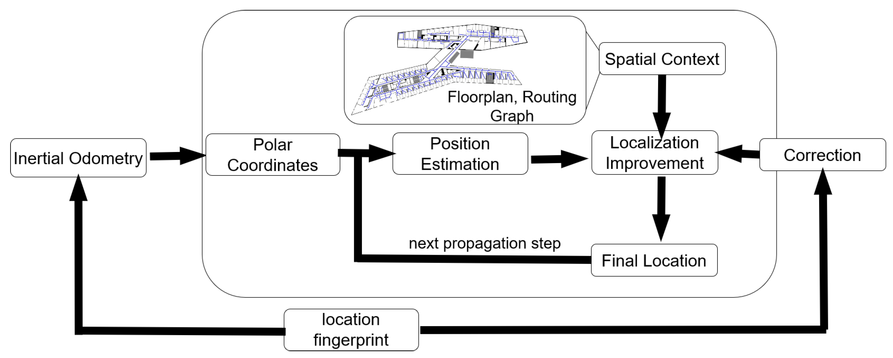In addition to the 5G correction in [29], here, further environmental information including, but not limited to, transition zones between floors (e.g., elevators or stairs) can be considered in combination with height information from barometer measurements. The overall high-level structure of the developed algorithm is shown in Figure 1. The polar coordinates (angle of orientation and traveled distance) used for the position estimation can be derived from different methods, such as PDR or odometry learning approaches. In this work, the focus has been on pedestrian navigation, and, for this reason, the polar coordinates are referred to as step headings (direction of movement as angle of orientation) and step lengths (traveled distance per time as the length of each step).

2. Methodology

This section describes and explains the underlying methodologies of this work, including geospatial analysis, the backtracking particle filter, and the corrections based on location fingerprints.

2.1. Geospatial Analysis

Geospatial analysis describes the process of extracting, manipulating, and visualizing spatial information [30]. One use case for geospatial analysis is the investigation of the spatial relationship between geometric objects. The most fundamental geometric objects are so-called geometric primitives. These are geometric objects that can be described by one continuous geometry and include points, curves, surfaces, and solids [31].

Geospatial analysis can be done with a variety of tools, including geographic information system (GIS)-software such as QGIS [32] or ArcGIS [33] or by using programming languages, for example Python, with libraries such as GeoPandas [34]. GeoPandas is an open-source project, extending the data types used by pandas to enable spatial analysis on geometric objects. These data types are GeoSeries and GeoDataFrames. The fundamental geometric objects are implemented in Shapely (as Point class), LineString class, and Polygon class. Several geometries of the same kind can be unified as collections, resulting in so-called MultiPoints, MultiLinestrings, and MultiPolygons [35]. GeoSeries and GeoDataFrames can store one or several different geometric objects. GeoDataFrames, which are basically extensions of the DataFrames used in the Python library Pandas, also enable the storage of attributes of geometric objects. This spatial data structure includes spatial relationships between geometric objects, such as contains, intersects, overlaps, touches, etc. Geometric operations, such as the investigations of the mentioned spatial relationships, are performed by Shapely [35]. Queries for spatial relations will return a Boolean value (True or False). Some queries for spatial relationships, implemented in Shapely, are listed below:

• Intersects returns True if the boundary or interior of the object intersect in any way with those of the other;
• Contains returns True if no points of the other geometry lie in the exterior of this geometry and at least one point of the other geometry’s interior lies in the interior of this geometry. A line’s endpoints are its boundary and are therefore not contained;
• Within returns True if this object’s boundary and interior intersect only with the interior of the other (not its boundary or exterior), making it the ‘inverse’ of contains;
• Touches returns True if the given objects’ boundaries have at least one point in common, but their interiors do not intersect with any part of the other.

The function of some of the fundamental geospatial analyses that can be applied to GeoSeries and GeoDataFrames are listed below and are shown in Figure 2:

• Distance returns the direct distance between geometries. It is also the orthogonal distance between a point and a line feature or edge, if the orthogonal projection of the point exists (see Figure 2a). Here, the distance from the corners of polygon B and the edges of the polygons A and C is simultaneously the orthogonal distance, whereas the distance between the corners of A and C is not);
• Spatial join is used to merge geometric objects based on their spatial relationships, as shown in Figure 2b. Spatial relationships, that can be used as requirements for the spatial join include intersects, contains, within, or touches;
• Query by attribute returns all objects of the given GeoDataFrame that hold the queried attribute value, as shown in Figure 2c, where all objects with the Type value of B are selected and marked in blue;
• Buffer generates a representation of all points in a given distance of the geometry as a polygon. In Figure 2d, the resulting buffer-polygons around a given line and a square-shaped polygon are displayed in green.

2.2. Backtracking Particle Filter

This section explains the principles of the backtracking PF. The idea of a PF in the application of navigation, specifically for PDR, is to approximate the PDF of the position by a large number of weighted, independent particles [27]. The weighted mean of the particles will then result in a position estimate.

When using a PF for positioning with map information support, paths can be estimated incorrectly. For example, a change in direction occurs at a location where there are several junctions close by. It can happen that the path follows the wrong junction, due to uncertainties in the positioning. The wrong path might lead to an aborting of the filter, due to strong corrections from the map information. If the scattering of the particles is wide enough, part of the particles might travel the correct path. In this case, a backtracking functionality can recalculate the path from the stored history of the movements of the particles.

In the following, such a backtracking PF, a variation of the PF model, is explained in detail. Many other variations of the PF exist, which mainly differ from each other by modifications of one or more of the components. For examples of other PF modifications, see [26,36], among others. A PF with backtracking works in its basic functionality similar to a simple bootstrap PF. However, compared to the bootstrap PF, it also considers the particle trajectory’s history to improve position estimates. As in the bootstrap PF, at first, a set of initial particles is created, representing the PDF of the starting position. The starting position can either be known or unknown. For the PDR, the particles are either all located at the known starting point, as in [9], or they can be distributed around the starting point according to the uncertainty of the position. In other cases, for example in combination with absolute positioning methods such as received signal strength indication RSSI, the particles could also be randomly distributed over the whole area, as done by [37]. The backtracking PF then consists of three steps: the propagation, filtering, and backtracking.

During the propagation step, the individual particles are changed to better represent the PDF. In pedestrian positioning, the particles can be spatially propagated according to the length and heading of the current step, which are derived from the odometry outputs. Possible measurement errors can be taken into consideration by assigning a randomly distributed noise to step length and step heading for each particle, as done by [9]. After the propagation, the trajectories of invalid particles, for example those that cross walls or non-accessible areas, are deleted during the so-called filtering step. Other approaches can be used, filtering the particles based on the distance to routing lines or based on the room that they are located in.

After the deletion of invalid particles in the filtering step, the position estimate is calculated from the mean of the particle positions and the orientation of the device is updated by the mean of the products of each particle’s noise value for the orientation and the measured orientation for the position. Optionally, the remaining valid particles can also be weighted according to spatial constraints, for example their distance to the closest routing edge. The weighted mean of these particles results then in the position estimate.

Next, for every particle that was deleted in the filter step, a new particle attempts to be generated within a specified and random radius around a valid particle. The potential new particle’s propagation history, according to the displacement of the steps, is then checked for their validity according to the above-mentioned filter methods. If the trajectory is valid, the particle is accepted, otherwise a particle with a different position and a different random scale for the displacement is proposed, as shown in Figure 3. During the backtracking segment of the PF, new particles are generated until the maximum number of particles is reached again.

2.3. Location Fingerprint

The location fingerprinting is a similar concept to the landmarks approach in map matching [13]. Contrary to other landmark approaches, where a dedicated graph of the location of specific features is created, here, only isolated information is used when possible to correct the position of particles. This can basically be any information that is detectable by the used device and is specific to a certain space. This could, for example, include position information from cellular networks, e.g., from a 5G campus network, as implemented in [29]. Another option can be to use the barometer in a smartphone to detect significant height changes that indicate that a user is using stairs or elevators and can, therefore, only be located in such.

3. Map Matching Based on a Backtracking Particle Filter

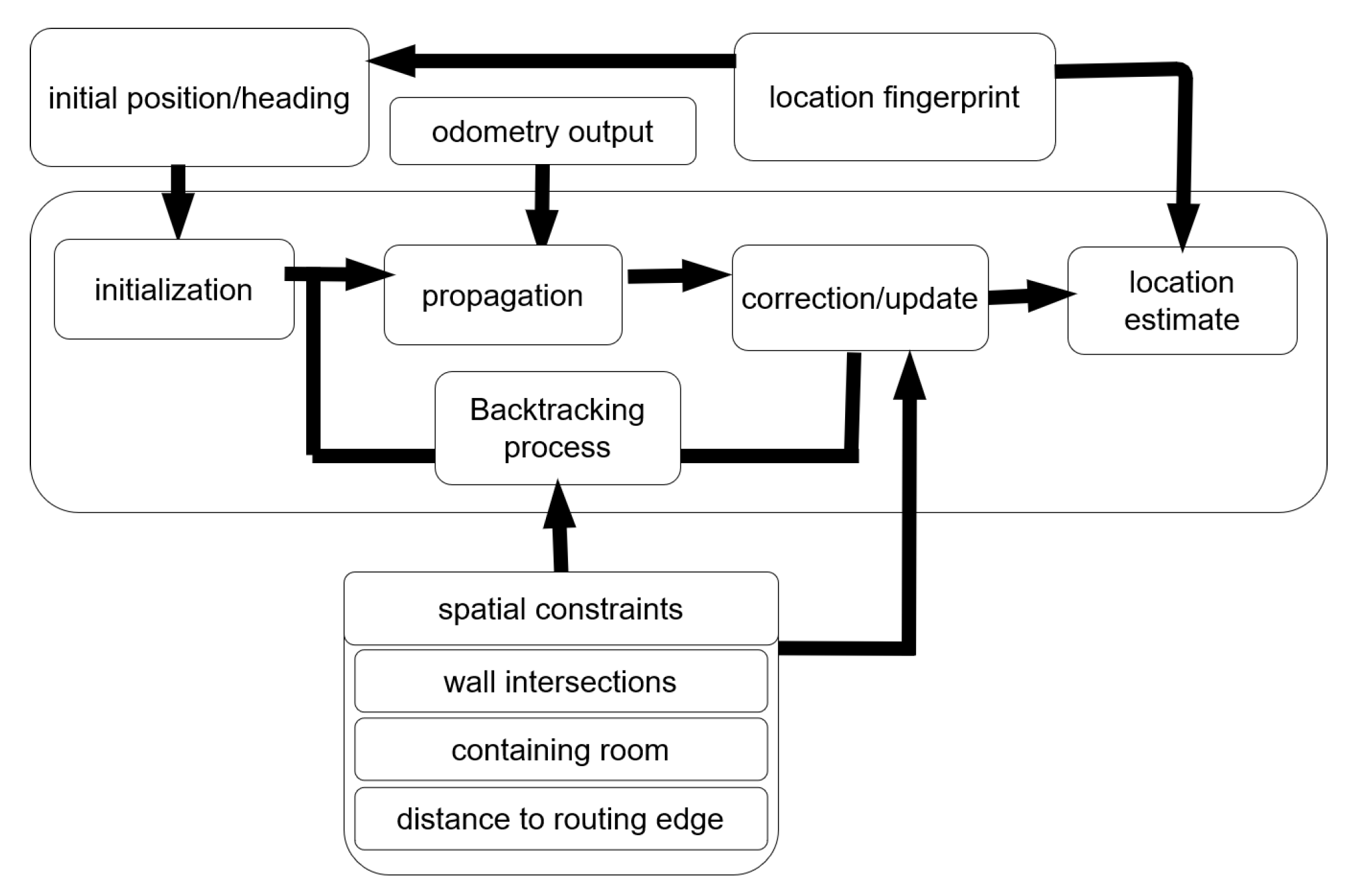
This section explains the implementation of the developed backtracking PF with geospatial analysis in the map-matching process. In Figure 4, a high-level overview of the developed map-matching process is presented.

The algorithm for the map matching is shown in Algorithm 1 as pseudo code. As input, it requires the odometry data, i.e., the step heading, step length, and step height, as well as the map information ($FloorData$). In line 2, the initial particles at the start position are created before the for-loop from line 3 on iterates over all steps while performing the map-matching processes. For every step, the current floor is determined and the floor data is selected accordingly (line 4 to 6).

Algorithm 1 Map-matching algorithm with backtracking PF

Input: $Startpoint,StepHeading,StepLength,StepHeight,FloorData$ Output: result 1: maxParticleNumber = 200 2: $particles\leftarrow \mathit{InitializeParticles}$(Start,maxParticleNumber,σH,σS) 3: fori in $StepNumber$ do 4:     $CurrentFloor\leftarrow \mathit{CheckFloor}$(Height) 5:     $FloorChanged\leftarrow True/False$ 6:     set $FloorData$ according to the $CurrentFloor$ 7:     $Step\leftarrow \mathit{Step}$ (StepLength,StepHeading,Height,CurrentFloor,CurrentConstraints, CurrentPosition,StepScale) 8:     $PropagatedParticles\leftarrow \mathit{CheckParticleSteps}$(particles,Step,FloorData) 9:      $weights\leftarrow \mathit{WeightingMethod}$(PropagatedParticles, FloorData) 10:    $PositionEstimate\leftarrow \mathrm{weighted}\mathrm{mean}\mathrm{of}particles\mathrm{positions}$ 11:     append $PositionEstimate$ to $Trajectory$ 12:     $NumberOfNewParticles\leftarrow maxParticleNumber-$                           number of $PropagatedParticles$ 13:     $particles\leftarrow \mathit{BackTracking}$(NumberOfNewParticles,PropagatedParticles,                          $BackTrackingSteps,FloorData,S$) 14:     return $PositionEstimate$ 15: return$Trajectory$

Next, a step-object ($Step$) is created (line 7), which stores the length, heading, height, current floor, the current position estimate, and the room it is located in, as well as all specific spatial constraints for this step (e.g., rooms where particles are allowed) for the current step. In line 8, the particles’ positions are then propagated based on the step length and step heading and are filtered regarding their plausibility according to the chosen filter concept. If the support through additional particle weights is active, the particles’ weights are determined according to the weighting method afterwards, otherwise all weights are set to one. The weighted mean of the particles’ position then provides the position estimate. Following the estimation of the position, the backtracking algorithm (Algorithm 2) is executed to create new particles and add them to the GeoDataFrame containing the propagated, valid particles. These are then used in the next loop of the backtracking PF algorithm. After the PF is performed on the last backtracking step, all calculated positions, as well as the standard deviation of each position estimate, is returned and saved as a comma separated values (CSV) file.

In this work, the initial particles are normally distributed around the starting position with a standard deviation of the uncertainty of the start position. The start position can be estimated from the location fingerprint, but it can also be set manually if a location fingerprint is not available. The initial heading of the user can be derived from the angle of the line fitted through the first few positions after the user starts to move in a chosen direction.

Algorithm 2 Backtracking Algorithm

Input: $particle,Steps,ValidRooms$ Output: $particles$ 1: $Samples\leftarrow \mathit{randomChoice}$(particles,NumberOfNewParticles) 2: forp in Samples do 3:     while $Try>0$ do 4:         $NewParticle\leftarrow \mathit{ProposeParticle}$(p,Radius) 5:         if BackTrackingTest($NewParticle$) is passed then 6:                  append $NewParticle$ to $particles$ 7:         $Try=Try-1$   return$particles$

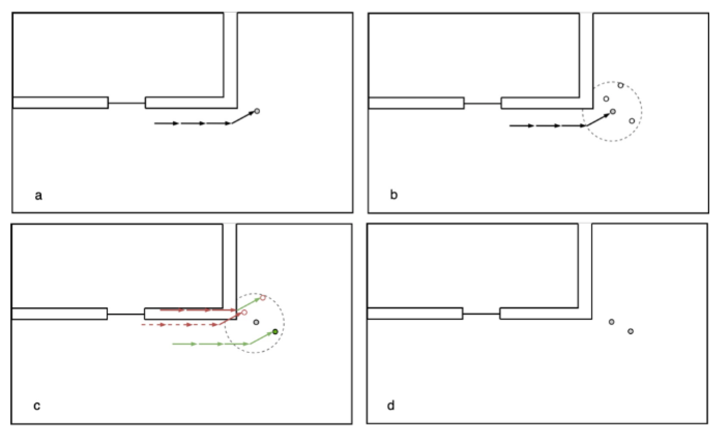
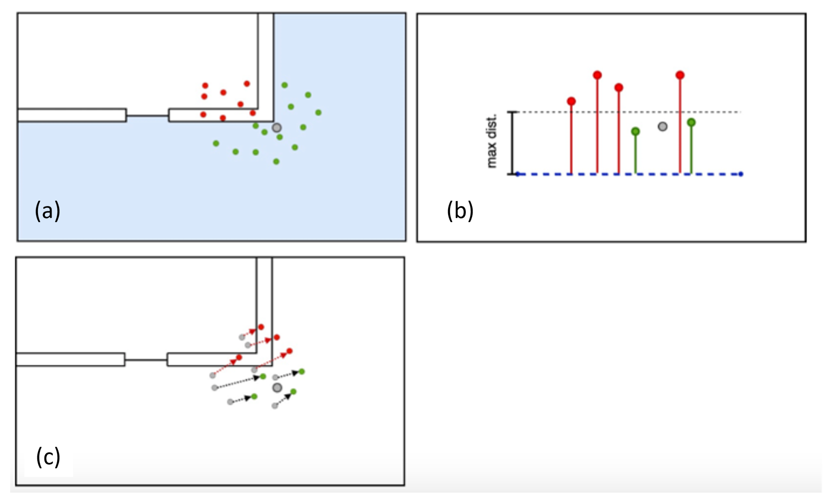
In the backtracking PF with geospatial analysis, the propagation of the particles is integrated in the filter process, in which the particles are checked for their plausibility by a specific concept. In this work, either the checking for line of sight (cl), checking for containing rooms (cm), or checking for distance to routing graph (cr) concept are used (see Figure 3), but other approaches could be implemented as well. The new position of each particle, $X_i,Y_i$, is calculated in the propagation step (see Figure 2) with Equations (1) and (2):

$$X_i=X_{last,i}+(S+{ϵ}_{l,i})\ast cos(H_0+H_{gy}+{ϵ}_{h,i})$$

(1)

$$Y_i=Y_{last,i}+(S+{ϵ}_{l,i})\ast sin(H_0+H_{gy}+{ϵ}_{h,i})$$

(2)

where $H_0$ is the initial heading, $H_{gy}$ is the estimated heading from the odometry data, S is the measured step length, and ${ϵ}_{l,i}$ and ${ϵ}_{h,i}$ are the noise values for the step length and step heading for each ith particle, respectively.

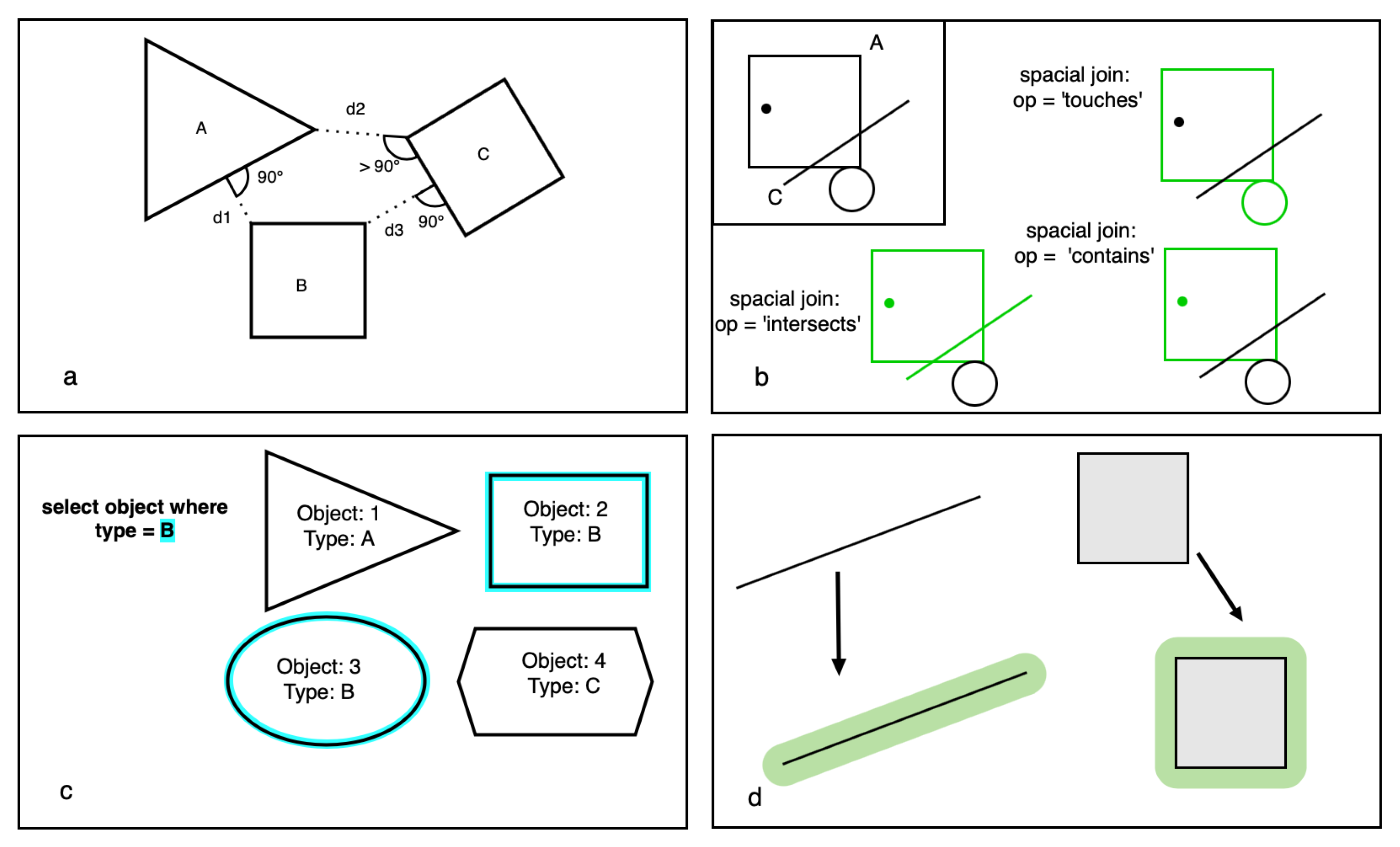
For this paper, three filtering methods for the validity of particles have been used, namely the checking by line of sight (cl), checking by rooms (cm), and checking by distance to the routing graph (cr) concept. For the cl (see Figure 3c), a GeoDataFrame is created containing all the connections between each propagated particle and its previous position. Every particle whose corresponding connection line intersects a wall is deleted, while all other particles are kept in the GeoDataFrame. Finally, the GeoDataFrame with the remaining particles is returned. The cm (see Figure 3a) concept is similar to cl. However, here, the walls are not required as map information, but the rooms, considered as valid for the particles ($ValidRooms$), and doors. For each propagated particle, it is checked if it is either within one of the valid rooms or if the LineString-geometry from its new and its previous position intersects either with any door-polygon or any polygon contained in $Transitions$. If that is the case, it is appended to the valid particles, which are finally returned as a GeoDataFrame. Rooms, which are entered by particles through doors are added to the list of valid rooms and kept valid as long as particles are inside them. In the cr concept (shown in Figure 5b), for each propagated particle, the smallest distance to the routing edges is determined. Only if the smallest distance to the routing edges for a particle is smaller than 2 m, is it then appended to the list of valid particles. The valid particles are then, as for the other concepts, returned as a GeoDataFrame.

The correction concept is implemented in the algorithms of the explained filtering methods. In this work, the location fingerprinting is based on floor changes. After the propagation of the particles, the height change over a defined number of recent steps is observed. If this height change exceeds a specified threshold, all particles that are not located in transition zones (stairs and lifts) connecting the current and the new floor are deleted. The remaining particles are then filtered according to the implemented filtering methods.

The underlying algorithm of the backtracking segment is presented in Algorithm 2. First, a number of particles, according to the difference between the number of valid particles and the maximum number of particles, is randomly chosen from the currently existing particles (line 2). For each sample particle, a new particle at a random position inside a specified radius (line 1) is proposed (line 5). For this proposed particle, a backtracking test (see Algorithm 3) is performed and, if it passes the test, it is appended to the existing particles (line 6 to 8). If the particle doesn’t pass the backtracking test, the procedure is repeated until either the maximum number of particles is reached or until a maximum number of tries (in this case eight tries) has been reached. The limited number of tries will prevent an unnecessary slowing down of the algorithm due to a very high number of tries for each particle. The GeoDataFrame, to which the accepted particles are added, is finally returned.

Algorithm 3 Backtracking test

Input: $particle,Steps,FloorData$ Output: $True/False$ 1: for each s in $Steps$ do 2:     propagate($particle,s$) 3:     if CheckValidity($particle,FloorData$)←valid then 4:         $continue$ with test 5:     else 6:         return $False$    return$True$

For each concept used for the checking of particles, the same concept is used for the backtracking test. For each backtracking step $i-1$, backwards from the current step i, the new position $X_{p,i-1},Y_{p,i-1}$ of each particle p is calculated from the current position of the particle $X_{p,i},Y_{p,i}$ with Equations (3) and (4):

$$X_{p,i-1}=X_{p,i}-(S_{i-1}+{ϵ}_{l,p})\ast cos(H_0+H_{gy,i-1}+{ϵ}_{h,p})$$

(3)

$$Y_{p,i-1}=Y_{p,i}-(S_{i-1}+{ϵ}_{l,p})\ast sin(H_0+H_{gy,i-1}+{ϵ}_{h,p})$$

(4)

where $S_{i-1}$ is the step length of the previous step and $H_{gy,i-1}$ is the heading of the previous step. Each backtracking step is then checked for its validity (intersections with walls for the cl, containing rooms for the cm, or distance to routing edges for cr). If the whole trajectory passes the backtracking test, the algorithm returns True, otherwise the algorithm returns False. When the cl concept is used, it is not checked for intersection at every step, but for all steps simultaneously because the query for intersections is the most time-consuming step and the usage of GeoDataFrames makes it more efficient to query for intersections of the LineString-geometry representing the whole trajectory than to query for intersections at each step if multiple steps are considered.

4. Test Data

The map matching based on the backtracking PF has been tested with the three different concepts, cl, cm, and cr, for the particle checks on two different trajectories. For the two test trajectories, the step length and orientation from PDR based on the smart phone’s INS was used. The used data sets, including the building information and the data for step heading, step length, and height is described in this section. The data has been provided by [29]. The sensor data as well as the floor plans are available on the GitHub platform, linked in the data availability statement section at the end of the article.

4.1. Building Information

The building information of the HafenCity University Hamburg (HCU) has been provided as floor plans in GeoJSON format, that was extracted from CAD plans [29] and have been minimally cleaned up manually. They contain polygons with attributes according to their type (e.g., walls, rooms, hallways, staircase, etc.). The floor plans have been provided separately for each, the ground floor, 1st floor, and 4th floor. The floor plans are loaded in the developed algorithm in GeoDataFrame structures, handled by the GeoPandas library. The complex architecture of the HCU building, including big, open hallways, small corridors, as well as unconventionally shaped rooms with pointy corners (see Figure 6), results in a distinct environment to test the developed PF under various conditions.

4.2. Sensor Data

The values for the step length and the step heading for the two tested trajectories, which have been estimated during a previous study of the authors [29], have been readily provided in the CSV format. The provided step headings are the orientation deviations in relation to the orientation at the starting point, making it necessary to add the absolute starting orientation to each heading value to derive the absolute heading to geographic north. The model for the step length calculation from the IMU values were based on a person with a different height and, therefore, a different step length than the persons who were generating the test data, which leads to a significant systematic error for the step length values. This provided a situation in which the robustness of the map-matching algorithm to systematic errors of the step length could be evaluated. The height difference for each step was also provided as a CSV file. To get the absolute height at any given step, the height differences until that step had to be summed up and added to the starting height. The starting height was approximated as the height of the starting floor plus 80% of the users’ height. The ground truth of the walked trajectories has been provided as a CSV-file as well and contains the horizontal position, time stamp, and the height difference for each point.

The height of the floors was estimated as 0 m for the ground floor, 6 m for the 1stfloor, and 19 m for the 4th floor. The two trajectories are referred to as eight path and zerotofour path in the rest of this thesis. The eight path starts in a corridor of the 4th floor in front of an office in the western direction and continues in the shape of an eight (see Figure 7 for the ground truth of the eight path).

The zerotofour path starts in the entrance hallway on the ground floor (Figure 8a) and leads over the main stairs to the 1st floor. It than takes a left turn and proceeds to take the elevator figure (Figure 8b) to the 4th floor. It continues along the corridor in the 4th floor southwards, then takes a turn at the t-junction and leads into an office room in the south-eastern part of the 4th floor (Figure 8c).

5. Results

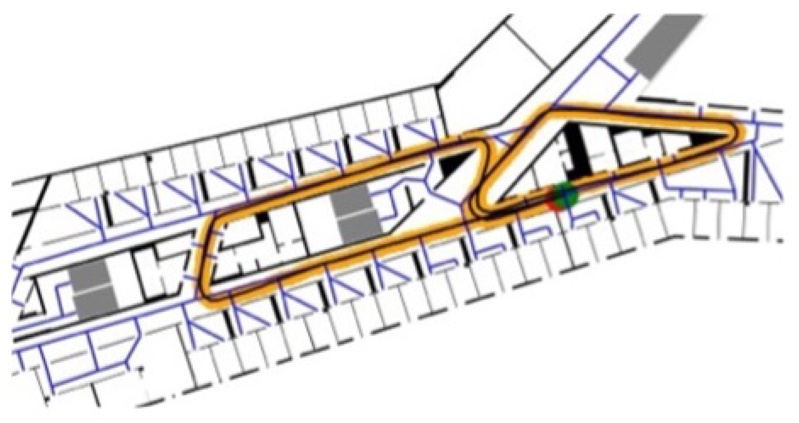
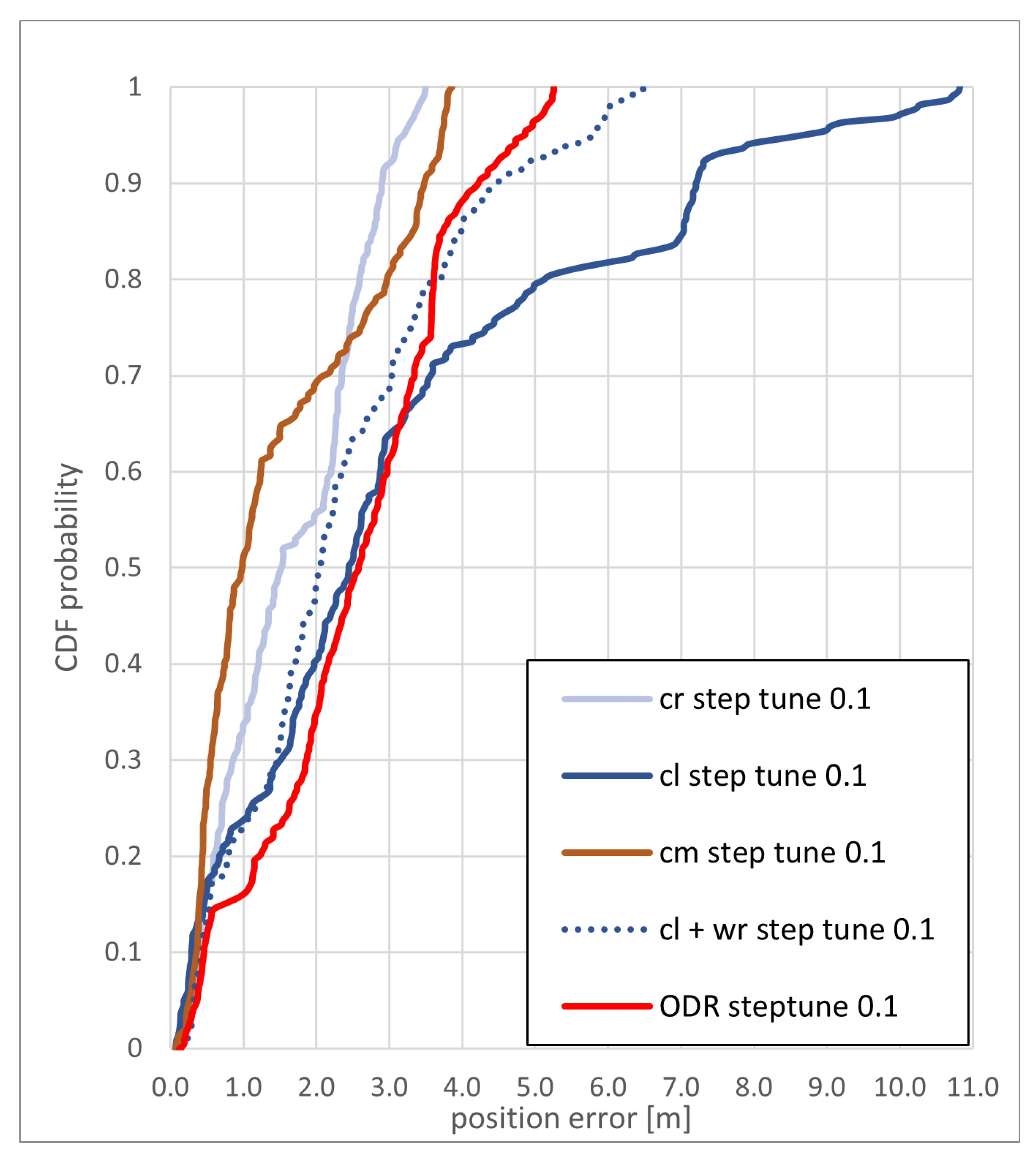
In this section, the results of the map-matching algorithm using the cr, cm, and cl method for particle checks are presented and discussed for the two test trajectories. The cumulative distribution function (CDF) of the position estimate error for the different concepts used for the eight path, with a step correction (manual step scale) of 0.1 m, is shown in Figure 9. The cm and cr method reached an overall similar accuracy, with the cm method reaching an accuracy of less than 4 m and the cr method reaching a accuracy of just less than 3 m in 90% of the steps.

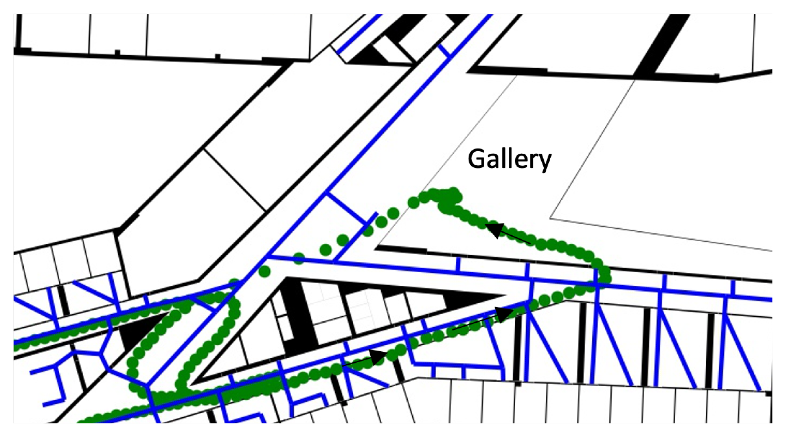
The cl method performed significantly worse; this is mainly due to the situation that at a step correction of 0.1 m, enough particles are overshooting at one of the turns, ending up in the “gallery” that the positions for the next steps is estimated to be on the wrong side of the wall (see Figure 10).

At this point, the backtracking functionality can be observed (see Figure 11). At the end of the “gallery”, with every subsequent step, more particles get deleted because they would cross a wall, resulting in the backtracking algorithm resampling the invalid particles at more plausible positions and by this, changing the trajectory to the correct path.

This was also an exception, where the weighting of the particles corresponding to the distance to the nearest routing edge helped to significantly increase the accuracy to less than 4.5 m in 90% of steps, by correcting the trajectory closer to the next routing edge (see Figure 12). Since the “gallery” does not contain any routing edges, the trajectory was directed back into the corridor. The effect of the weighting method was negligible for the other methods for the tested trajectories.

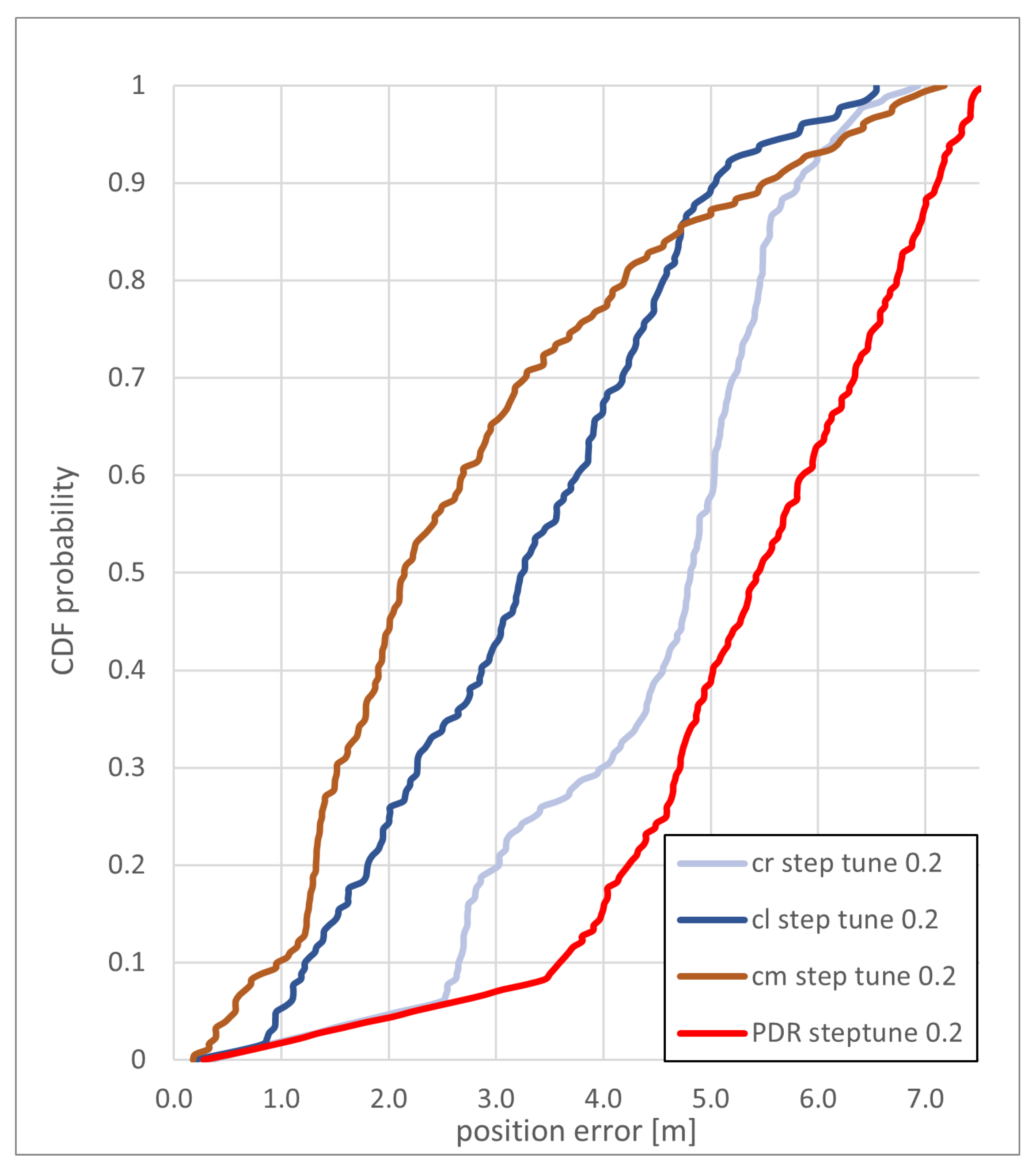
Figure 13 shows the CDF of the position estimate error for the zerotofour path with a step correction of 0.2 m. The accuracy for all methods is between 5 and 6 m in 90% of the steps. The cm method can provide a position error of less than 4 m more often than the two other methods. From the three methods, only the cm method lead the trajectory into the elevator, while only the cr method reached the final room. The cm and the cl method both lead the trajectory into the neighboring room, west of the final room.

For the eight path without step correction, an accuracy better than 3 m can be achieved with the cm and cl method, while the overall performance of the cr method falls behind the two other methods, as shown in Figure 14. The use of additional routing support worsens the achievable accuracy of the cr method. For the cm and cl method, the weighting by the distance to the routing graph has only a small influence on the error of position estimate. The cl method performs significantly better (also see Figure 15), mainly because there is less particle overshoot at the turn at the eastern corner. This way, the trajectory doesn’t deviate into the “gallery”.

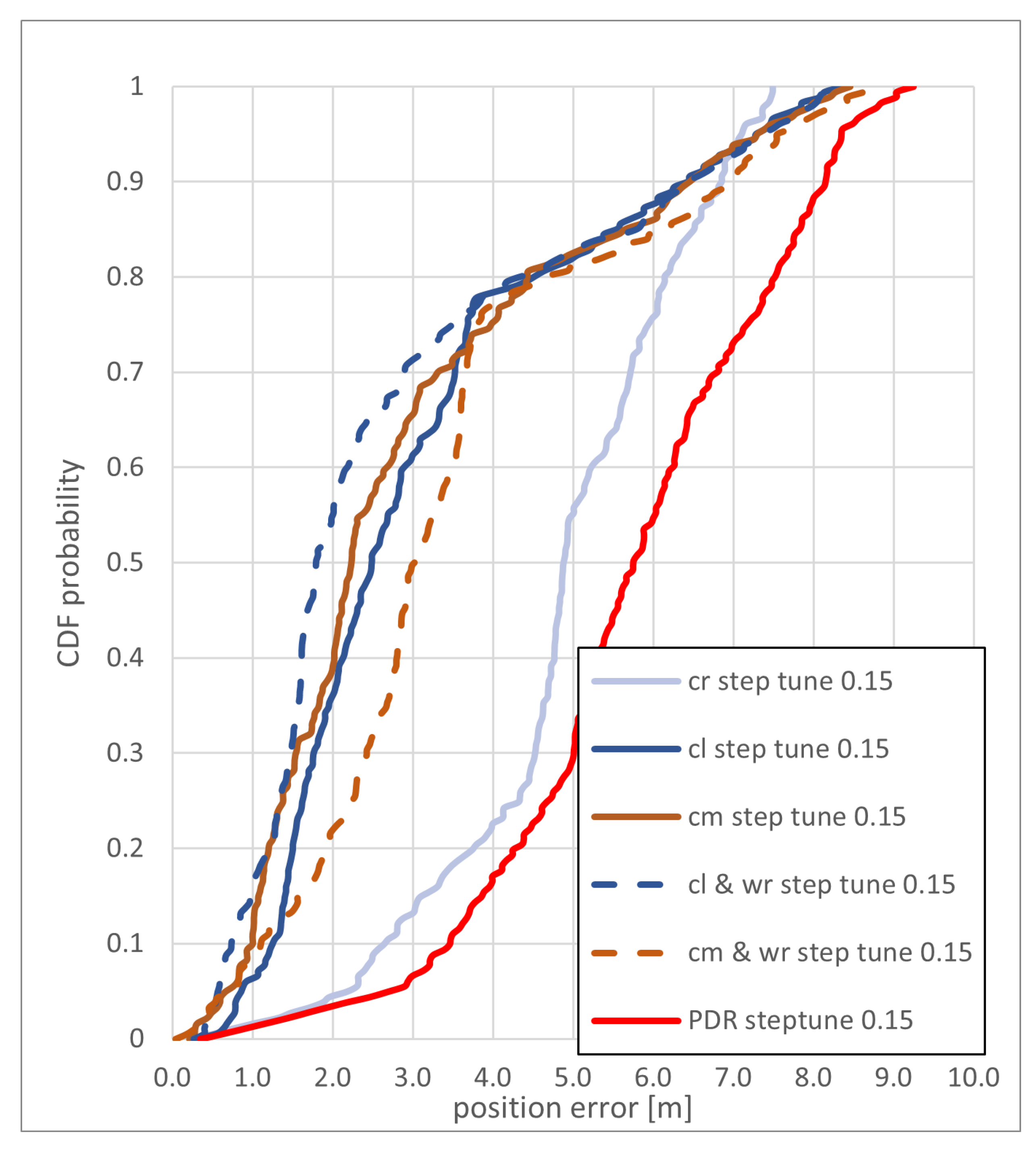
Figure 16 shows the different method’s CDF of the positioning error for the zerotofour path with a step length correction of 0.15 m. All methods, with and without the additional use of the weighting method, achieve a positioning error of less than 7 m in 90% of the steps, while the cm and cl methods achieve a significantly better accuracy for the positioning than the cr method. The additional weighting of particles only has a minor influence on the accuracy of the used methods, slightly improving the cl method and slightly decreasing the accuracy of the cm method. The elevator could be reached by the cl method as well as the cl and cm methods with routing support. It was closely missed by the cm method. The cr method was the only one that reached the destination room, with all the other trajectories ending in the same neighboring room.

In most cases, the cm and the cl method had the best accuracy. The eight path with a step correction of 0.1 m is the exception; here, the cl method reached a significantly worse accuracy, due to the above mentioned situation in which the trajectory gets “trapped” in the gallery for a part of the trajectory.

6. Conclusions

Fitting the odometry outputs with spatial information is a way to correct for the cumulative noises. In this paper, a real-time map-matching method based on a backtracking PF has been developed that can handle different odometry inputs. It provides flexibility to use different kinds of spatial constraints due to the usage of geospatial analysis tools and can be implemented in different use cases. We could successfully develop a PF algorithm that autonomously supports a meter scale position accuracy for indoor navigation. We took the benefits of both odomotery and geospatial anaylsis to develop and evaluate possible algorithms that can provide map-matching services for any kind of moving object. For this, first the underlying concepts and methodology were explained and related work was presented. Next, the concepts as they were further developed and adjusted for this paper have been explained, including the detailed explanation of the implementation of the algorithms of the backtracking PF. Finally, the used test data set was presented and the results of the backtracking PF with geospatial analysis have been investigated and discussed. In addition, a simple correction method has been developed and implemented that can use additional environmental information to further improve the position estimate. In this paper, the height information from a smartphone was used to determine if a user is located on stairs or in elevators in order to develop a simple corrector/optimizer by these transition zones. An extended optimization can be done with other position information, e.g., cellular positioning such as 5G, for a continuous correction. Three methods were developed that determine invalid particles based on different building information, namely the cl, cm, and cr method. The results of the different methods have been tested with the data from two paths through the HCU building and have been compared with regard to the attainable position accuracy, as well as the ability to detect certain rooms.

The cm and cl methods reached better precision than the cr method, with the cm method being a bit more robust. It was possible to develop a PF algorithm that could reach an accuracy of 2 to 7 m most of the time in the two tested trajectories. Of all the tested methods, the cm method for particle checking might be favorable, not only because its performance regarding the position precision and room accuracy, but also because additional information for the accessibility of rooms can be relatively easily implemented. n broken elevator could, for example, easily be declared as an invalid space.

Due to the simple and modular code structure, it is possible to add or exchange methods and functionalities to the developed map-matching algorithm. This would also include the additional use of position estimation, for example from 5G antennas, for the correction method. Since polar coordinates are used for the propagation model, in this case, step length and step heading, the usage is not limited to pedestrian navigation, but the developed approach could also be implemented for other use cases such as the indoor navigation of robots or any other moving object, as long as the traveled distance (which can easily be calculated from the speed) and moving direction is provided. Compared to conditional random fields, a PF does not need learning data, making it more convenient and versatile to use in a variety of real-life scenarios. To improve the accuracy in situations where large hallways provide only few possibilities for map corrections, position information from cellular networks (e.g., 5G) could be used in the implemented correction approach to improve the accuracy (see [29]).

The accuracy of the developed PF approaches is dependent on the quality of the provided map information, resulting in better performances with better map materials. The quality of the step length estimation could be improved either by scaling the step length every time an absolute position can be attained with high precision and accuracy, either through infrastructure support or when a position is determined with relatively high confidence regarding their correctness; for example, when using an elevator changes the floor. This could be implemented during the implemented correction method. On the other hand, machine-learning algorithms could be used for a more precise step length estimation. Another option would be to use data sets of step length in relation to other biometric information from a huge number of people. However, these are costly and hard to attain. Overall, a novel map-matching algorithm, based on a backtracking PF, has been developed that provides a meter scale accuracy and is applicable in a large variety of use cases and can easily be modified to handle different kinds of spatial information in different scenarios.

References

1. Willemsen, T.; Keller, F.; Sternberg, H. Kartengestützte MEMS-basierte Indoor-positionierung mittels Partikel Filter. In Oldenburger 3D-Tage; Photogrammetrie-Laserscanning Optische 3D-Messtechnik Th. Luhmann/Ch. Müller (Hrsg.), Wichmann, VDE Verlag GmbH, Berlin and Offenbach: Oldenburg, Germany, 2015; ISBN 9783879075287. [Google Scholar]
2. Winter, S. Indoor spatial information. Int. J. 3-D Inf. Model. 2012, 1, 25–42. [Google Scholar] [CrossRef]
3. Wang, H.; Sen, S.; Elgohary, A.; Farid, M.; Youssef, M.; Choudhury, R.R. No need to war-drive: Unsupervised indoor localization. In Proceedings of the 10th International Conference on Mobile Systems, Applications, and Services, Applications, and Services, Windermere, UK, 25–29 June 2012; pp. 197–210. [Google Scholar]
4. Li, F.; Zhao, C.; Ding, G.; Gong, J.; Liu, C.; Zhao, F. A Reliable and accurate indoor localization method using phone inertial sensors. In Proceedings of the 2012 ACM Conference on Ubiquitous Computing, Pittsburgh, PA, USA, 5–8 September 2012; pp. 421–430. [Google Scholar] [CrossRef]
5. Lewandowicz, E. Network models of 2D and 3D carastral data. In Proceedings of the 9th International Conference on Environmental Engineering, ICEE 2014, Vilnius, Lithuania, 22–23 May 2014. [Google Scholar] [CrossRef]
6. Shoushtari, H.; Willemsen, T.; Sternberg, H. Many ways lead to the goal—Possibilities of autonomous and infrastructure-based indoor positioning. Electronics 2021, 10, 397. [Google Scholar] [CrossRef]
7. Yang, J.; Cao, Z.; Zhang, Q. A fast and robust local descriptor for 3D point cloud registration. Inf. Sci. 2016, 346, 163–179. [Google Scholar] [CrossRef]
8. Dubé, R.; Dugas, D.; Stumm, E.; Nieto, J.; Siegwart, R.; Cadena, C. SegMatch: Segment based place recognition in 3D point clouds. In Proceedings of the 2017 IEEE International Conference on Robotics and Automation (ICRA), Singapore, 29 May–3 June 2017; pp. 5266–5272. [Google Scholar] [CrossRef] [Green Version]
9. Willemsen, T. Fusionsalgorithmus zur Autonomen Positionsschätzung im Gebäude, Basierend auf MEMS-Inertialsensoren im Smartphone. Ph.D. Thesis, HafenCity Universität Hamburg, Hamburg, Germany, 2016. [Google Scholar]
10. White, C.E.; Bernstein, D.; Kornhauser, A.L. Some map matching algorithms for personal navigation assistants. Transp. Res. Part C Emerg. Technol. 2000, 8, 91–108. [Google Scholar] [CrossRef]
11. Lan, K.C.; Shih, W.Y. On calibrating the sensor errors of a PDR-based indoor localization system. Sensors 2013, 13, 4781–4810. [Google Scholar] [CrossRef] [PubMed] [Green Version]
12. Park, J.G.; Teller, S. Motion Compatibility for Indoor Localization; Technical Report; Massachusetts Institute of Technology: Cambridge, MA, USA, 2014. [Google Scholar]
13. Gu, F.; Valaee, S.; Khoshelham, K.; Shang, J.; Zhang, R. Landmark Graph-Based Indoor Localization. IEEE Internet Things J. 2020, 7, 8343–8355. [Google Scholar] [CrossRef]
14. Xiao, Z.; Wen, H.; Markham, A.; Trigoni, N. Lightweight map matching for indoor localisation using conditional random fields. In Proceedings of the 13th International Symposium on Information Processing in Sensor Networks (IPSN-14), Berlin, Germany, 15–17 April 2014; pp. 131–142. [Google Scholar]
15. Bataineh, S.; Bahillo, A.; Díez, L.E.; Onieva, E.; Bataineh, I. Conditional Random Field-Based Offline Map Matching for Indoor Environments. Sensors 2016, 16, 1302. [Google Scholar] [CrossRef] [PubMed] [Green Version]
16. Thiagarajan, A.; Ravindranath, L.; LaCurts, K.; Madden, S.; Balakrishnan, H.; Toledo, S.; Eriksson, J. Vtrack: Accurate, energy-aware road traffic delay estimation using mobile phones. In Proceedings of the 7th ACM Conference on Embedded Networked Sensor Systems, Berkeley, CA, USA, 4–6 November 2009; pp. 85–98. [Google Scholar]
17. Newson, P.; Krumm, J. Hidden Markov map matching through noise and sparseness. In Proceedings of the 17th ACM SIGSPATIAL International Conference on Advances in Geographic Information Systems, Seattle, WA, USA, 4–6 November 2009; pp. 336–343. [Google Scholar]
18. Ma, Y.; Dou, Z.; Jiang, Q.; Hou, Z. Basmag: An optimized HMM-based localization system using backward sequences matching algorithm exploiting geomagnetic information. IEEE Sens. J. 2016, 16, 7472–7482. [Google Scholar] [CrossRef]
19. Wu, Y.; Chen, P.; Gu, F.; Zheng, X.; Shang, J. HTrack: An efficient heading-aided map matching for indoor localization and tracking. IEEE Sens. J. 2019, 19, 3100–3110. [Google Scholar] [CrossRef]
20. Peter, M.; Fritsch, D.; Schafer, B.; Kleusberg, A.; Link, J.A.B.; Wehrle, K. Versatile geo-referenced maps for indoor navigation of pedestrians. In Proceedings of the International Conference on Indoor Positioning and Indoor Navigation (IPIN), Sydney, Australia, 13–15 November 2012; pp. 1–4. [Google Scholar]
21. Davidson, P.; Collin, J.; Takala, J. Application of particle filters for indoor positioning using floor plans. In Proceedings of the 2010 Ubiquitous Positioning Indoor Navigation and Location Based Service, Kirkkonummi, Finland, 14–15 October 2010; pp. 1–4. [Google Scholar]
22. Woodman, O.; Harle, R. Pedestrian localisation for indoor environments. In Proceedings of the 10th International Conference on Ubiquitous Computing, Seoul, Korea, 21–24 September 2008; pp. 114–123. [Google Scholar]
23. Yu, C.; Lan, H.; Gu, F.; Yu, F.; El-Sheimy, N. A map/INS/Wi-Fi integrated system for indoor location-based service applications. Sensors 2017, 17, 1272. [Google Scholar] [CrossRef] [PubMed]
24. Gu, F.; Hu, X.; Ramezani, M.; Acharya, D.; Khoshelham, K.; Valaee, S.; Shang, J. Indoor localization improved by spatial context—A survey. ACM Comput. Surv. 2019, 52, 64. [Google Scholar] [CrossRef] [Green Version]
25. Wendel, J. Integrierte Navigationssysteme; Oldenbourg Verlag: München, Germany, 2011; ISBN 9783486704396. [Google Scholar] [CrossRef]
26. Aggarwal, P.; Syed, Z.; El-sheimy, N.; Noureldin, A. MEMS-Based Integrated Navigation; Artech House: Norwood, MA, USA, 2010. [Google Scholar]
27. Gordon, N.J.; Salmond, D.J.; Smith, A.F.M. Novel approach to nonlinear/non-Gaussian Bayesian state estimation. In IEE Proceedings F-Radar and Signal Processing; IET: London, UK, 1993; Volume 140, pp. 107–113. [Google Scholar]
28. Widyawan; Klepal, M.; Beauregard, S. A Novel Backtracking Particle Filter for Pattern Matching Indoor Localization. In Proceedings of the First ACM International Workshop on Mobile Entity Localization and Tracking in GPS-Less Environments (MELT ’08), San Francisco, CA, USA, 19 September 2008; Association for Computing Machinery: New York, NY, USA, 2008; pp. 79–84. [Google Scholar] [CrossRef]
29. Shoushtari, H.; Askar, C.; Harder, D.; Willemsen, T.; Sternberg, H. 3D Indoor Localization using 5G-based Particle Filtering and CAD Plans. In Proceedings of the International Conference on Indoor Positioning and Indoor Navigation (IPIN), Lloret de Mar, Spain, 29 November–2 December 2021. [Google Scholar] [CrossRef]
30. Cappelli, C. The Language of Spatial Analysis; Esri Press: Redlands, CA, USA, 2013; Available online: https://www.esri.com/content/dam/esrisites/sitecore-archive/Files/Pdfs/library/books/the-language-of-spatial-analysis.pdf (accessed on 1 July 2021).
31. Peuquet, D. A Conceptual Framework and Comparison of Spatial Data Models. Cartogr. Int. J. Geogr. Inf. Geovis. 1984, 21, 66–113. [Google Scholar] [CrossRef] [Green Version]
32. QGIS Development Team. QGIS. QGIS Webpage. Available online: http://qgis.osgeo.org (accessed on 3 April 2022).
33. Redlands, CA: Environmental Systems Research Institute (ESRI). ArcGIS. ArcGIS Webpage. Available online: www.esri.com (accessed on 3 April 2022).
34. Developers, G. Geometric Manipulations. GeoPandas Documentation. Available online: https://geopandas.org/docs/user_guide/geometric_manipulations.html (accessed on 2 July 2021).
35. Gills, S. The Shapely User Manual. 2021. Available online: https://shapely.readthedocs.io/en/latest/manual.html#binary-predicates (accessed on 2 July 2021).
36. Arulampalam, M.S.; Maskell, S.; Gordon, N.; Clapp, T. A tutorial on particle filters for online nonlinear/non-Gaussian Bayesian tracking. IEEE Trans. Signal Process. 2002, 50, 174–188. [Google Scholar] [CrossRef] [Green Version]
37. Real Ehrlich, C.; Blankenbach, J. Indoor localization for pedestrians with real-time capability using multi-sensor smartphones. Geo-Spat. Inf. Sci. 2019, 22, 73–88. [Google Scholar] [CrossRef] [Green Version]
Figure 1. Overview of the structure of the developed algorithm that uses particle filtering as a map-matching process. Starting from a position derived, for example, through a location fingerprint, odometry data from inertial measurements are transferred to polar coordinates, resulting in the estimation of the propagated position. This estimation is improved via spatial constraints and further corrected by additional information from the location fingerprint, resulting in the final position estimate, which serves as the starting point for the next propagation step.
Sensors 22 03289 g001
Figure 2. Overview of some of the geospatial analyses used in GeoPandas, with distance shown in (a), spatial join in (b), query by attribute in (c), and buffer in (d).
Sensors 22 03289 g002
Figure 3. Overview of the backtracking process. A particle with valid trajectory is randomly chosen (a). Particles are randomly created in a specified radius (b). Newly created particles with invalid trajectories (red) are discarded until a particle with a valid trajectory (green) is found (c) and is accepted as a new particle (d).
Sensors 22 03289 g003
Figure 4. Overview of the particle filter algorithm. The initial position and heading, derived from the location fingerprint, is used for the initialization of the particles, which are then propagated according to the odometry output. The particles are then filtered in the correction/update according to spatial constraints, leading to a final location estimation, which is further improved by the location fingerprint. Via the backtracking process, the number of valid particles is increased up to the original amount of particles by considering spatial constraints. Next, the next propagation step starts.
Sensors 22 03289 g004
Figure 5. Overview of the used filtering methods, with the cm in (a), cr in (b), and cl in (c).
Sensors 22 03289 g005
Figure 6. Floor plans of the ground floor (a), 1st floor (b), and 4th floor (c), with the blue lines representing the routing edges.
Sensors 22 03289 g006
Figure 7. Ground truth points (orange) of the “eight path”; the red dot is the starting position and the green dot is the finish.
Sensors 22 03289 g007
Figure 8. Ground truth points (orange) of the zerotofour path in (ac); the red dot is the starting position and the green dot is the finish.
Sensors 22 03289 g008
Figure 9. CDF of the positioning error of the eight path with a step length correction of 0.1 m for the backtracking PF and the PDR with a step length correction of 0.1 m.
Sensors 22 03289 g009
Figure 10. Part of the trajectory of the eight path, that wrongly proceeds in the “gallery”, when using the weighting by routing support method, where black arrows indicate the walking direction and the green points represent the position estimates for each step.
Sensors 22 03289 g010
Figure 11. Example of the trajectory correction (from (ad)) through the backtracking functionality, where the green dots represent the valid, propagated particles, and the blue dot is the resulting position estimate. First, most particles took a “wrong” path (a), continuously getting deleted when trying to pass the wall (ac). While more particles are getting deleted, more particles with plausible trajectories are getting created through the backtracking process, until all particles are recovered and now only represent positions with reasonable trajectories again (d).
Sensors 22 03289 g011
Figure 12. Effect of the support through the weighting by routing support on the deviated trajectory.
Sensors 22 03289 g012
Figure 13. CDF of the positioning error of the zerotofour path with a step length correction of 0.2 m for the backtracking PF and the PDR with a step length correction of 0.2 m.
Sensors 22 03289 g013
Figure 14. CDF of the positioning error of the eight path without step length correction for the backtracking PF and the PDR without step length correction.
Sensors 22 03289 g014
Figure 15. Trajectory (green dots) from the cl method for the eight path without step length correction for the backtracking PF.
Sensors 22 03289 g015
Figure 16. CDF of the positioning error of the zerotofour path with a step length correction of 0.15 m for the backtracking PF and the PDR with a step length correction of 0.15 m.
Sensors 22 03289 g016
Publisher’s Note: MDPI stays neutral with regard to jurisdictional claims in published maps and institutional affiliations.