Abstract
The accurate prediction of photovoltaic (PV) power is essential for planning power systems and constructing intelligent grids. However, this has become difficult due to the intermittency and instability of PV power data. This paper introduces a deep learning framework based on 7.5 min-ahead and 15 min-ahead approaches to predict short-term PV power. Specifically, we propose a hybrid model based on singular spectrum analysis (SSA) and bidirectional long short-term memory (BiLSTM) networks with the Bayesian optimization (BO) algorithm. To begin, the SSA decomposes the PV power series into several sub-signals. Then, the BO algorithm automatically adjusts hyperparameters for the deep neural network architecture. Following that, parallel BiLSTM networks predict the value of each component. Finally, the prediction of the sub-signals is summed to generate the final prediction results. The performance of the proposed model is investigated using two datasets collected from real-world rooftop stations in eastern China. The 7.5 min-ahead predictions generated by the proposed model can reduce up to 380.51% error, and the 15 min-ahead predictions decrease by up to 296.01% error. The experimental results demonstrate the superiority of the proposed model in comparison to other forecasting methods.
1. Introduction
With the rapid development of modern society, global energy production and demand have increased dramatically [1]. However, traditional energy stocks are limited, and carbon dioxide emissions during combustion can cause environmental problems, including global warming and the greenhouse effect. As a result, the adjustment of the energy structure and the development and utilization of new energy sources have gradually attracted the attention of all countries in the world [2]. Solar energy is a clean, green, sustainable, and renewable energy source. In the case of falling costs, the penetration rate of solar energy in the energy market is gradually increasing [3].
In recent years, solar PV power plants have been widely used because of their intense power generation capacity. However, the random, volatile, and intermittent nature of PV power data causes the grid system to face significant issues such as stability, reliability, and power balance. Accurate short-term PV power forecasting plays a vital role in the security, stability, and economic operation of the power grid and the dispatching plan of PV power systems [4]. Therefore, numerous studies have been conducted on PV power prediction, with a brief survey provided in the rest.
In [5], a review of PV power forecasting models is given. PV power forecasting techniques mainly include persistence forecast methods, physical models, statistical techniques, machine learning forecast techniques, and deep learning strategies. Persistence models suggest that today’s solar irradiance is similar to the day before [6]. However, if weather conditions change considerably, persistence methods often fail. Physical techniques rely on the current weather service data and satellite image data. Aguiar et al. [7] used NWP and satellite data to forecast Spain’s global horizontal irradiance. Moreover, physical models do not require historical PV data but use specific weather characteristics. Similarly, false forecasts occur when the values of weather variables change suddenly. In [8], a step-by-step method based on the autoregressive moving average (ARMA) is proposed for PV power prediction for the next hourly time horizon. However, statistical techniques are limited in handling large amounts of data. Machine learning algorithms are applied to time series data forecasting. Kaushika et al. [9] were the first to apply the feedforward neural network (FFNN) algorithm to the field of PV power prediction using weather information. In [10], a novel model based on neural networks and multilayer perceptrons used a least squares optimization algorithm to predict the next 24 h. Huang et al. [11] proposed a data-driven framework that fuses the spatiotemporal information of target and neighboring PV sites. The multi-step ahead prediction of solar irradiance showed that boosted regression trees are more suitable than the benchmark model.
Various deep learning (DL) methods have recently been introduced for time series data forecasting issues. However, the temporal dependencies in PV power generation data are not considered by artificial neural networks (ANNs). Meanwhile, the advantage of deep learning techniques is that they have a significant capacity for nonlinear data. LSTM has been applied to time series data prediction issues [12], air quality forecasting [13,14], load forecasting [15], and solar irradiation forecasting [16,17], to name a few. Numerous prediction experiments have demonstrated how different data pretreatment techniques significantly boost the neural network model’s capacity for prediction [18]. In [13], a multitask multi-channel nested LSTM (NLSTM) hybrid deep learning framework combining stationary wavelet transform (SWT) was proposed to forecast air quality. In comparison to support vector machines (SVM), Yan et al. [19] asserted that LSTM neural networks perform better at capturing the dependencies between data samples. They proposed a novel DL forecasting framework combining cutting-edge LSTM and the widely used SWT. In another study, Yan et al. [20] applied a multichannel extension LSTM model to forecast energy consumption from data collected in London, UK. Jin et al. [21] proposed a deep learning model based on singular spectrum analysis and LSTM for 5 min energy consumption forecasting. In [22], a support vector regression (SVR) model with a convolutional neural network gated recurrent unit (CNNGRU) network was designed. The SSA algorithm was used to decompose the raw wind speed data. The proposed method was evaluated using three verification datasets. Barbieri et al. [23] developed a novel method for predicting very short-term PV output using satellite and sky imaging. Furthermore, it implies that hybrid models can improve forecast accuracy. Yao et al. [4] proposed an innovative deep learning-based forecasting system incorporating an improved U-net and an encoder–decoder architecture. Several experiments are provided to discuss the ideal framework configuration and structure. It achieved maximum error reductions of 4.561% and 3.55% in terms of RMSE and MAE. Ren et al. [24] applied an accurate intra-hour PV power forecasting model with the quad-kernel deep convolutional neural network (CNN) for case studies from a 26.52 kW PV plant. Yan et al. [25] developed a CNN-LSTM integrated model for short-term load forecasting at multi-step predicted horizons. Zang et al. [26] created a hybrid model to predict PV power using the two-dimensional CNN method, resulting in a lower forecast error across multiple evaluation criteria. In another study [27], PV power generation was forecasted for time horizons ranging from 7.5 min-ahead to 60 min-ahead by combining the LSTM model with the attention mechanism. The attention mechanism adaptively focuses on more significant input features when taking into account how temperature data affect PV power generation. The prediction effect outperforms the comparison model in each time domain. In [28], a hybrid LSTM convolutional model was presented to forecast the PV power 5 min in advance. The fusion order influences the model’s prediction accuracy and time consumption significantly. The LSTM-CNN model outperforms CNN-LSTM in terms of performance and computational time. In [29], an effective PV power forecasting framework was developed based on wavelet analysis and LSTM with a stochastic differential equation to provide accurate prediction information in different seasons. Pi et al. [16] used multichannel wavelet transform combining CNN and BiLSTM networks to forecast solar irradiance under different time horizons. Shah et al. [30] forecasted electricity price and demand successfully, and the Diebold and Mariano test was used to determine the statistical significance of differences in model performance. According to the current literature, the data decomposition algorithm with LSTM offers the excellent capability to handle volatile and intermittent data.
As might be deduced from the justifications above, PV power forecasting has drawn academic attention recently. However, deep neural network (DNN) creation is a laborious iterative process that involves both technical knowledge and trial-and-error experience. Additionally, tuning the DNN hyperparameters is crucial since the network performance’s effectiveness is highly related to its architecture [17]. It can be inferred from studying prior research in the area of PV power forecasting that most of these studies manually constructed deep structures through trial and error. This process is quite difficult computationally due to the long execution time of a tailored architecture. Thus, this paper proposes a method to automatically produce accurate predictions of PV power without manually tuning the deep learning architectures [31,32]. Zhou et al. [33] developed a PV forecasting framework with a signal decomposition technique and a multi-objective chameleon swarm algorithm to predict short-term PV power. The R-square scores obtained from Safi-Morocco are 0.995, 0.993, and 0.995, respectively. The performance of the time series can be improved based on the optimization algorithm. To this end, a combinatorial model that combines the SSA and optimized architecture of BiLSTM with BO is proposed to create a highly reliable model. In conclusion, the main contributions of this paper are as follows:
- (1)
- A neural network structure composed of several parallel BiLSTM neural networks. Each BiLSTM is used to train the corresponding sub-signal produced by the SSA. The integrated approach enables more precise prediction by processing multiple sub-signals, potentially improving the final prediction accuracy.
- (2)
- Applying the Bayesian optimization algorithm in PV power prediction. Bayesian optimization is considered to search hyperparameters for LSTM. The proposed Bayesian optimization algorithm enhances the prediction performance of LSTM.
- (3)
- A novel artificial intelligence forecasting framework that combines SSA and parallel BiLSTM neural networks. The SSA is intended for denoising and feature extraction to improve prediction performance. The SSA outputs are fed in parallel to a series of BiLSTM neural networks.
- (4)
- A comprehensive comparative study. We compare the proposed SSA-BO-BiLSTM with cutting-edge technologies, including machine learning methods and various extensions of LSTM. The experimental results show that the proposed model outperforms the existing models in terms of effectiveness and efficiency.
2. Methodology
This section illustrates the details of the proposed PV power hybrid forecasting framework. Firstly, the PV power series is decomposed into stationary sub-signals with a singular spectrum analysis algorithm [34]. Then, the parameters of the BiLSTM model are tuned using the Bayesian optimization algorithm. Subsequently, the BiLSTM neural network is connected to each sub-signal for forecasting. Finally, we presented the overall architecture of the proposed model.
2.1. Singular Spectrum Analysis
Singular spectrum analysis is a nonparametric time series decomposition method that combines the time and frequency domains [22,35]. SSA can extract the intrinsic driving characteristics of sequence fluctuations and denoise original PV power data. The SSA technique is utilized to preprocess data by signal decomposition. Light coral represents the original signal, and blue represents the decomposition signal, as shown in Figure 1. Compared to the initial time series data, the decomposed sub-signals are more regular, effectively reducing the difficulty of prediction. Such a strategy demonstrates its potential to improve the forecasting performance of BiLSTM neural networks.
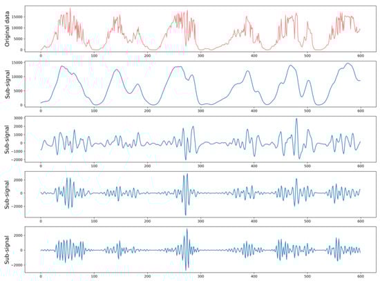
Figure 1.
SSA decomposed several subsequences of the original time series.
SSA includes decomposition and reconstruction stages [36]. The decomposition stage includes two sub-processes of embedding and singular value decomposition. The reconstruction stage includes two sub-processes of grouping and diagonal averaging. The detailed steps of the SSA can be explained in the following subsections:
2.1.1. Embedding
Assuming the original time series with F observations, the original one-dimensional Y = [y1, y2, …, yF]T is converted into a multi-dimensional time series by the sliding window method with embedded dimension L, then there is a trajectory matrix X as follows (1):
where K = F − L + 1, 2 ≤ L ≤ F/2. i = 1, 2, …, K is called the L-lagged vector.
2.1.2. Singular Value Decomposition
Let S = XXT. Denote λ1, λ2, …, λL as the values of the matrix S, and the corresponding eigenvector is U1, U2, …, UL. The singular value denoises the original signal. Additionally, matrix X is decomposed using (2):
where U, V, and Σ are the left matrix, right matrix, and diagonal matrix, respectively.
2.1.3. Sequence Grouping
Divide index I = (1, 2, …, d) into p groups I1, I2, …, IP with no intersection. Define I = (i1, i2, …, im) for each group, and the corresponding result matrix is XI = Xi1 + Xi2 + ⋯ + Xim. Trajectory matrix X is converted by using the following (3):
2.1.4. Diagonal Averaging
Let M = L × K, Mij is the element of matrix M, where 1 ≤ i ≤ L, 1 ≤ j ≤ K. The diagonal average converts M into a sequence {M1, M2, …, MF}, given as (4):
where L* = min(L, K), K* = max(L, K). The original sequence yi can be decomposed as (5):
2.2. Bayesian Optimization
Hyperparameter optimization enhances the performance of deep neural networks. The parameter tuning methods include experimental trial-and-error methods, a grid search, and a random search. However, these methods have some shortcomings. For example, the experimental trial-and-error method is time-consuming and not always optimal for the performance of the network. Grid search is inefficient even with parallel computing. Past work has shown that random search is more efficient than grid search [32], but the problem is that it is easy to miss accurate solutions. In contrast to traditional methods, Bayesian optimization generates every guess based on previous training results. It requires fewer iterations and has a higher computational speed. More importantly, Bayesian optimization remains robust when dealing with nonconvex problems and is less likely to fall into local optima.
Bayesian optimization uses the probabilistic model surrogate function to fit the objective function [37,38]. Then, the following hyperparameter combination is chosen to sample based on the posterior probability distribution. Let α = α1, α2, …, αn be a set of hyperparameter combinations, f (α) is the objective function of the hyperparameter α. The principle of Bayesian optimization is to find that α belongs to U such that:
In other words, the algorithm aims to find the optimal parameter set by minimizing the loss value L while making the generalization error as small as possible. The steps of Bayesian optimization are as follows:
- (1)
- A Gaussian process (GP) calculates the posterior probability distribution. The GP is a set of random variables in which any linear combination of finite samples has a joint Gaussian distribution. GP is represented by the mean function m and the covariance matrix function k as follows in (7):
- (2)
- Apply the upper confidence bound (UCB) method to determine the next sample location. μ represents development, model uncertainty σ represents exploration, and k is the hyperparameter that can control the focus of development and exploration. Avoid local optima by making a trade-off between exploration and exploitation.
- (3)
- Output suitable hyperparameters.
2.3. BiLSTM Neural Network
In recurrent neural networks, the influence of long-term historical information on the output at the current moment decreases with the passage of the sequence, and the problem of gradient disappearance occurs. The hidden layer of the LSTM replaces simple neurons with complex memory modules and retains historical information more reliably [12].
Figure 2 shows the memory module structure of the BiLSTM network. The memory module consists of forget gate Ft, input gate It, and output gate Ot. Ft (9) decides which information to discard at the current moment through the sigmoid function. It (10) decides which information needs to be updated through the sigmoid layer, (11) generates alternative cell state new information through the tanh layer. After the forgetting and input links are completed, the long-term memory is updated. Ot (13) determines what information will be output to the next layer of LSTM. At the current time t, the final output ht (14) is defined by the current cell state Ct (12) and the output gate Ot.
where W denotes the corresponding weight, and b represents the corresponding bias values. [,] is the joining of two matrices, is the multiplication of the related elements of the matrix, and is the matrix addition operator. σ and tanh are activation functions.
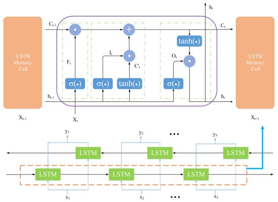
Figure 2.
The internal structure of the BiLSTM unit.
One-way LSTM cannot obtain past and future information at the same time. As shown in Figure 2, BiLSTM inputs the time series forwards and reverses to two LSTM memory modules. The outputs of the two modules are jointly sent to the output layer, which effectively solves the information timing problem.
2.4. Hybrid Forecasting Model
In this paper, an artificial intelligence (AI) model for short-term PV power forecasting is proposed. Figure 3 shows the details of the AI model architecture. The whole process can be described in five steps as given below:
- Step 1:
- The original data should be preprocessed before being input into the model. Firstly, the Augment Dickey–Fuller (ADF) test is used to determine whether the data are stationary. If the result is refused, differential processing is needed. Then, missing values are handled. We follow the principle of taking the mean of the previous and next rows of outliers. Last but not least, we utilize the Z-Score to standardize the raw PV power time series with an average value of 0 and a standard deviation of 1.
- Step 2:
- The processed data are decomposed into four sub-signals by implementing the SSA process. These decomposed signals exhibit much more stable behavior. The sub-signals are split training sets, validation sets, and testing sets. Take the data of 87.5% as the training set, the training set of 5% as the validation set, and the data of 12.5% as the testing set.
- Step 3:
- The Bayesian optimization algorithm is used to select appropriate parameters. It is noteworthy that parameters are an important issue in LSTM, which need to be given in advance. In this study, LSTM is trained using Bayesian optimization to enhance the predictor’s performance.
- Step 4:
- Forecasting each sub-signal with BiLSTM. The sub-signals are the input of the parallel BiLSTM neural network. After training, the testing dataset is utilized to obtain the predicted results. Subsequently, denormalization of the forecasting results is performed.
- Step 5:
- Perform assessment functions to measure the prediction performance of PV power in terms of goodness of fit and error severity.

Figure 3.
Illustration of the SSA-BO-BiLSTM prediction strategy.
3. Experimental Process and Results
3.1. Data Description and Analysis
The original PV power generation data are collected from July to September 2017 and July to November 2016 from a roof PV power plant in eastern China. The dataset [29] is accessible from the Power and Energy datasets of IEEE DataPort. Each dataset is 7.5 min intervals of PV power. The measurement of the sensor data lasts approximately 12 h from sunrise to night. Table 1 provides the statistical information for each dataset.

Table 1.
Statistical information description of the PV power dataset.
For PV power dataset 1, 7000 data samples and 1000 data samples are used for training and testing, respectively. Then, 350 validation data are extracted from the training data. Similarly, PV power dataset 2 is divided into 11,200 data samples, 1600 data samples, and 560 data samples as the training test, testing test, and validation test, respectively.
The diagram of dataset 1 shows a clear demonstration in Figure 4 [39,40]. Figure 4a depicts the entire 7.5 min-ahead historical PV power generation data. Figure 4b plots PV power data from the first week of July 2017. A detailed observation of PV power on 1 July 2017, is shown in Figure 4c. The figures show that the data first rose at noon to reach the peak of power generation and then declined during the day. This trend is repeated every day, and the pattern is similar. Figure 4d depicts the first differential result from dataset 1. As we can see, after the first-order difference, the average value of the data returns to zero, indicating an inevitable stability trend. Table 1 presents the results of the ADF test and Ljung–Box (LB) test. Firstly, we performed the ADF test to check the stability of the PV power time series. The test statistic is less than the critical value of 1% (−3.43), 5% (−2.86), and 10% (−2.57) in the three confidence intervals. The p-value is less than 0.05 or equal to zero. Therefore, dataset 1 and dataset 2 are stationary series. Secondly, we used the Ljung–Box (LB) test to determine the randomness of the PV power time series. Each p-value of the white noise test is less than 0.05, indicating that the datasets are all nonwhite noise sequences. Thirdly, we performed missing value processing and data standardization. In addition, a fixed-size window slides across the raw PV power dataset [41]. We used the values in the window as the training input vector and the PV power at the next moment as the training target, respectively. During the test, we used the power value in the current sliding window as model input to predict the PV power at the next moment.
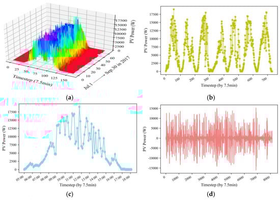
Figure 4.
PV power generation data. (a) The whole dataset in three dimensions, (b) Weekly frequency for the years 1 July 2017–7 July 2017, (c) A detailed observation of PV power in 1 July 2017, (d) The first different result of the whole dataset.
3.2. Experimental Setup
All programming work is completed on TensorFlow-GPU 2.6.0 and Keras 2.3.1. The hardware configurations are an AMD Radeon (TM) graphics CPU and an NVIDIA GeForce RTX 3050 Ti laptop GPU. The software environment is Python 3.7.0 on the Win11 system.
A three-step comparison is completed in this work. Firstly, we selected several classic machine learning methods, including decision tree, random forest, support vector regression, and multilayer perceptron. Secondly, we explored the effects of the Bayesian optimization algorithm on the LSTM neural network. Finally, we compared the performance of the proposed SSA–BiLSTM method with multiple LSTM extension hybrid models with data decomposition algorithms, including SWT, VMD, and SSA.
Four evaluation metrics, namely mean absolute error (MAE), root mean square error (RMSE), adjusted coefficient of determination (Adj-R2), and accuracy (ACC), are used in the experiment. Table 2 shows the equation for those criteria. It should be mentioned that the lower the MAE and RMSE values are, the higher the Adj-R2 and ACC values, and the more accurate the model forecasts.
Table 2.
Formulas of the accuracy metrics.
3.3. Hyperparameter Searching
The basic structure of the LSTM model consists of hidden layers, fully connected layers, and output layers in this study. RMSProp is employed to optimize the weights and biases in the LSTM network. The change in parameters may lead to different prediction performances. Hence, a hyperparameter search is performed based on Bayesian optimization, including the number of hidden layer units, the number of fully connected layer units, the learning rate, and the decay. The hyperparameter ranges are listed in Table 3.
Table 3.
The range of hyperparameters.
New ensemble hyperparameters can be selected with the UCB method. The root mean squared error is calculated as a loss function. The total number of iterations is 20. Through iterations of Bayesian optimization, the best set of hyperparameters will be used to build the final predictive neural network model. Table 4 shows the iterative process of these four hyperparameters in dataset 1. The loss function reaches a minimum at the 14th iteration. The set of hyperparameters will be chosen in the LSTM model to predict the PV power dataset 1.
Table 4.
Hyperparameter searching result.
The training and valid loss curves of the BO-LSTM model are shown in Figure 5, which show no symptoms of overfitting or underfitting. Figure 6 shows the fitted graph for LSTM and BO-LSTM based on historical data. The case indicates that the BO algorithm in PV power systems significantly affects the prediction effect. This means that the BO-based LSTM neural network forecast model can achieve a higher accuracy due to an efficient way to train the neural networks.
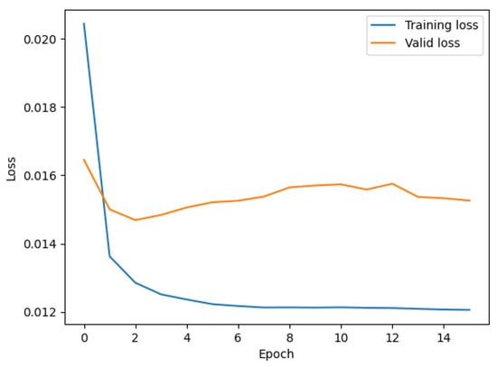
Figure 5.
The training and validation loss curves of the BO-LSTM model.
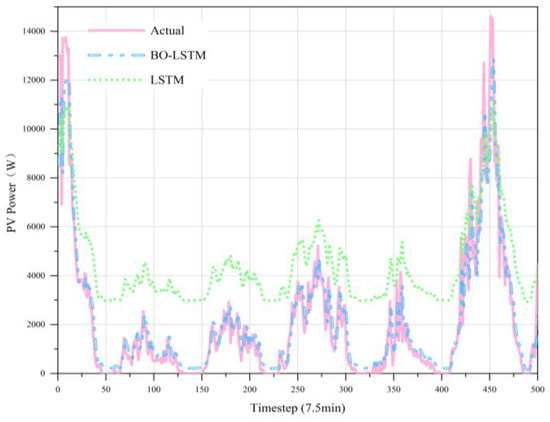
Figure 6.
Forecast results of PV power in dataset 1.
3.4. Results of the Experiment
The forecasting results of PV power produced by all the contrast methods with four evaluation metrics are given in Table 5 and Table 6, including MAE, RMSE, Adj-R2, and ACC. Table 5 reports the results of PV power prediction on dataset 1. These results illustrate that the proposed method outperforms all compared methods in terms of four evaluation metrics. From Table 5, we can see that the proposed method obtains the best results 7.5 min-ahead with values of 3.18 and 4.72 for the MAE and RMSE metrics, respectively. In addition, the MAE of the proposed method is reduced by 199.37% and 111.12% compared with the worst-performing model and reduced by 51.26% and 17.90% compared with the best-performing model, respectively. Similarly, the RMSE can obtain an identical conclusion. Adj-R2 is raised from 0.766 to 0.984 and 0.747 to 0.971, respectively. The Adj-R2 fitting effect is greatly improved. Similarly, the forecasting accuracy of the proposed algorithm rises sharply. Additionally, it is noted that the RMSE and MAE increase and the Adj-R2 and ACC values decrease for all the contrast methods from 7.5 min-ahead to 15 min-ahead. The experimental results on dataset 2 are shown in Table 6. Compared with thirteen existing prediction methods, the SSA-BiLSTM model performs best in different timesteps. For example, with 7.5 min-ahead horizon forecasting, the MAE, RMSE, Adj-R2, and ACC metrics have values of 3.60, 6.42, 0.975, and 74.23%, respectively. The proposed method is the best value among all the compared models. The SWT-NLSTM model places at the second-best position by obtaining the values of 3.93, 7.32, and 0.967 for MAE, RMSE metrics, and Adj-R2, respectively. Additionally, the performance of the algorithm is further verified. From one-step to two-step, the amount of error forecast by all methods increases, which means it is more challenging to predict PV power.
Table 5.
Performance comparison of different prediction methods based on dataset 1.
Table 6.
Performance comparison of different prediction methods based on dataset 2.
In summary, we have compared the machine learning methods, including DTR, RF, SVR, and MLP. The proposed model is compared with the LSTM model, the nested LSTM (NLSTM) model [43], and the bidirectional LSTM (BiLSTM) model [45]. The proposed and compared methods also use data decomposition techniques, namely, SWT [19], VMD [46], and SSA [47]. From the experimental results shown in Table 7, the mean MAE of the prediction error of LSTM and its extended model is 11.48, and the RMSE is 17.37. For the model using the SWT algorithm, the mean MAE of the prediction error is 8.76, and the RMSE is 14.18. It improves by 31.05% and 22.50%, respectively. Similarly, using the VMD algorithm model, the year-on-year increases were 18.72% and 24.43%, respectively. Compared to SWT and VMD, DL models combined with SSA perform more accurate predictions and produce less error. For the model using the SSA algorithm, the mean prediction error MAE is 6.18, and the RMSE is 9.25. Compared with the LSTM class model, it is improved by 85.76% and 87.78%, respectively. The forecast results indicate that the proposed method outperforms the existing compared methods in terms of efficiency and effectiveness.
Table 7.
The mean MAE and RMSE of various methods.
Figure 7, Figure 8, Figure 9, Figure 10 and Figure 11 reveal the actual values of the PV power and their forecasted values obtained by the proposed method and other methods. The forecast results of the proposed method and all compared methods of 7.5 min-ahead prediction for dataset 1 are displayed in Figure 7. The predicted and actual values of the proposed model neural network framework better fit not only during the rise or fall of the load but also during the peak and valley of the load. As seen in Figure 8, machine learning algorithms have significant lag effects. Figure 9 shows that the single LSTM model and its extended learning ability are insufficient, and there are obvious prediction errors. In Figure 10, the model adopting VMD to decompose PV power data is less efficient than the proposed model. Figure 11 shows that the SWT has low accuracy in predicting small fluctuations. Some peaks show the opposite trend. As shown in Figure 7 and Figure 11, compared with the proposed SSA, the SWT embedded model is too smooth and less accurate in predicting small fluctuations in PV power data. Some of the peaks have opposite trends, resulting in untimely and insignificant predictions.
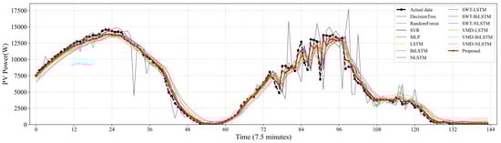
Figure 7.
Contrasting the final prediction result with the actual value.
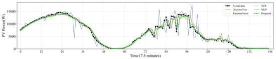
Figure 8.
Contrasting the performance evaluation of the proposed model and machine learning models.
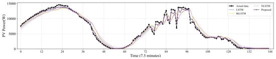
Figure 9.
Contrasting the performance evaluation of the proposed model and LSTM and extensions.
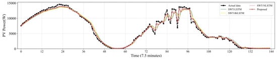
Figure 10.
Contrasting the performance evaluation of the proposed model and LSTM networks combining SWT.
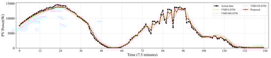
Figure 11.
Contrasting the performance evaluation of the proposed model and LSTM networks combining VMD.
Table 8 shows the training time for different forecasting algorithms. It is highlighted that the training time for ML models is short. Therefore, these models are not reported. The training time of the proposed DL model is completed in 159 s or less, which has high practicability. Additionally, the boxes of the absolute error of the proposed method and the contrast methods are shown in Figure 12. The proposed method has a lower average absolute error (AE) and narrower distribution. This means that the predicted values are more accurate and reflect the actual value consistently.
Table 8.
Training time in seconds for different forecasting models.
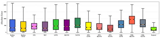
Figure 12.
The absolute error of the proposed model and the compared methods.
4. Discussion
From the experimental results, the following information can be obtained:
- (1)
- The lengths of the forecast horizons have negative impacts on the performance of the prediction methods.
- (2)
- The Bayesian optimization algorithm can improve the forecasting accuracy of deep neural networks.
- (3)
- Decomposition-based hybrid methods are superior to most single methods.
- (4)
- Most of the outperformance is achieved with the unique BiLSTM neural network. It obtains the forward and backward characteristics of PV power data. This approach enables the experimental results to be predicted more accurately by providing more thorough feature information. Although NLSTM also improves the prediction accuracy with the SWT decomposition method, the computational time of the NLSTM training process is significantly longer than BiLSTM. Therefore, the BiLSTM model is more suitable for PV power forecasting.
- (5)
- VMD decomposes the original PV power data to obtain modal functions of various frequencies, mainly divided into trend and fluctuation components. However, raw PV power data usually exhibit unstable and irregular properties. VMD is effective at predicting trends but poorly fitted at the cutting edge.
- (6)
- SWT analyses the local variations in the raw data using a local and adaptively long wavelet. The SWT decomposition technique lacks further analysis of high-frequency sub-signals. As a result, models incorporating SWT are insensitive to high-frequency fluctuations.
- (7)
- The PV power record is full of frequent and dramatic fluctuations. The characteristics of the dataset mean that SSA is more suitable for decomposing PV power data. On the one hand, the original signal is decomposed into several sub-signals. Each BiLSTM is used to train the corresponding sub-signal generated by the SSA. The learning sub-signal is conducted separately, increasing DL networks’ attention to every part of the data features. On the other hand, this processing eliminates the influence of data noise and has high noise immunity. The summation of the sub-signal prediction results during the training process is optimized. It can help to mitigate insensitivity to peak prediction issues.
5. Conclusions
In this paper, we have proposed a data-driven framework called SSA-BO-BiLSTM to predict PV power. In the architecture of the proposed SSA-BO-BiLSTM, the SSA is used for both denoising and feature extraction; the parallel BiLSTM is designed to predict the corresponding PV power sub-signal. In addition, we applied the Bayesian optimization algorithm to select hyperparameters for the deep BiLSTM architectures. Furthermore, the prediction vectors of the sub-signals are summed to bring about the final forecasting results. The efficiency of SSA-BO-BiLSTM is verified through experiments on real datasets with PV power under 7.5 min-ahead and 15 min-ahead forecasting scenarios. Case studies revealed that the proposed SSA-BO-BiLSTM model outperforms other cutting-edge methods in terms of MAE, RMSE, R2, and ACC metrics. In future work, we plan to explore a general model for load forecasting for different power stations. Therefore, we intend to securely leverage data from multiple parties with federated learning and transfer learning.
Author Contributions
Data curation, K.Y.; Methodology, X.G.; Resources, Y.M.; Software, X.G.; Validation, Y.M. and K.Y.; Writing—original draft, X.G.; Writing—review and editing, Y.M. and K.Y. All authors have read and agreed to the published version of the manuscript.
Funding
This work was supported in part by the China National Natural Science Foundation under Grant 61972165.
Institutional Review Board Statement
Not applicable.
Informed Consent Statement
Not applicable.
Data Availability Statement
The required datasets for the experiment can be obtained for free from https://dx.doi.org/10.21227/9hje-dz22 aeecssed on 17 May 2022.
Conflicts of Interest
The authors declare no conflict of interest.
References
- Huang, J.; Zhang, H.; Peng, W.; Hu, C. Impact of Energy Technology and Structural Change on Energy Demand in China. Sci. Total Environ. 2021, 760, 143345. [Google Scholar] [CrossRef] [PubMed]
- Rasheed, R.; Rizwan, A.; Javed, H.; Yasar, A.; Tabinda, A.B.; Bhatti, S.G.; Su, Y. An Analytical Study to Predict the Future of Pakistan’s Energy Sustainability versus Rest of South Asia. Sustain. Energy Technol. Assess. 2020, 39, 100707. [Google Scholar] [CrossRef]
- Das, U.K.; Tey, K.S.; Seyedmahmoudian, M.; Mekhilef, S.; Idris, M.Y.I.; Van Deventer, W.; Horan, B.; Stojcevski, A. Forecasting of Photovoltaic Power Generation and Model Optimization: A Review. Renew. Sustain. Energy Rev. 2018, 81, 912–928. [Google Scholar] [CrossRef]
- Yao, T.; Wang, J.; Wu, H.; Zhang, P.; Li, S.; Xu, K.; Liu, X.; Chi, X. Intra-Hour Photovoltaic Generation Forecasting Based on Multi-Source Data and Deep Learning Methods. IEEE Trans. Sustain. Energy 2022, 13, 607–618. [Google Scholar] [CrossRef]
- Ahmed, R.; Sreeram, V.; Mishra, Y.; Arif, M.D. A Review and Evaluation of the State-of-the-Art in PV Solar Power Forecasting: Techniques and Optimization. Renew. Sustain. Energy Rev. 2020, 124, 109792. [Google Scholar] [CrossRef]
- Jiang, Y.; Long, H.; Zhang, Z.; Song, Z. Day-Ahead Prediction of Bihourly Solar Radiance with a Markov Switch Approach. IEEE Trans. Sustain. Energy 2017, 8, 1536–1547. [Google Scholar] [CrossRef]
- Aguiar, L.M.; Pereira, B.; Lauret, P.; Díaz, F.; David, M. Combining Solar Irradiance Measurements, Satellite-Derived Data and a Numerical Weather Prediction Model to Improve Intra-Day Solar Forecasting. Renew. Energy 2016, 97, 599–610. [Google Scholar] [CrossRef]
- Singh, B.; Pozo, D. A guide to solar power forecasting using ARMA models. In Proceedings of the 2019 IEEE PES Innovative Smart Grid Technologies Europe (ISGT-Europe), Bucharest, Romania, 29 September–2 October 2019; pp. 1–4. [Google Scholar]
- Kaushika, N.D.; Tomar, R.K.; Kaushik, S.C. Artificial Neural Network Model Based on Interrelationship of Direct, Diffuse and Global Solar Radiations. Sol. Energy 2014, 103, 327–342. [Google Scholar] [CrossRef]
- Mellit, A.; Pavan, A.M. A 24-h Forecast of Solar Irradiance Using Artificial Neural Network: Application for Performance Prediction of a Grid-Connected PV Plant at Trieste, Italy. Sol. Energy 2010, 84, 807–821. [Google Scholar] [CrossRef]
- Huang, C.; Wang, L.; Lai, L.L. Data-Driven Short-Term Solar Irradiance Forecasting Based on Information of Neighboring Sites. IEEE Trans. Ind. Electron. 2019, 66, 9918–9927. [Google Scholar] [CrossRef]
- Hochreiter, S.; Schmidhuber, J. Long Short-Term Memory. Neural Comput. 1997, 9, 1735–1780. [Google Scholar] [CrossRef] [PubMed]
- Jin, N.; Zeng, Y.; Yan, K.; Ji, Z. Multivariate Air Quality Forecasting with Nested Long Short Term Memory Neural Network. IEEE Trans. Ind. Inf. 2021, 17, 8514–8522. [Google Scholar] [CrossRef]
- Zeng, Y.; Chen, J.; Jin, N.; Jin, X.; Du, Y. Air Quality Forecasting with Hybrid LSTM and Extended Stationary Wavelet Transform. Build. Environ. 2022, 213, 108822. [Google Scholar] [CrossRef]
- Shah, I.; Jan, F.; Ali, S. Functional Data Approach for Short-Term Electricity Demand Forecasting. Math. Probl. Eng. 2022, 2022, 6709779. [Google Scholar] [CrossRef]
- Pi, M.; Jin, N.; Chen, D.; Lou, B. Short-Term Solar Irradiance Prediction Based on Multichannel LSTM Neural Networks Using Edge-Based IoT System. Wirel. Commun. Mob. Comput. 2022, 2022, 1–11. [Google Scholar] [CrossRef]
- Jalali, S.M.J.; Ahmadian, S.; Kavousi-Fard, A.; Khosravi, A.; Nahavandi, S. Automated Deep CNN-LSTM Architecture Design for Solar Irradiance Forecasting. IEEE Trans. Syst. Man Cybern. Syst. 2022, 52, 54–65. [Google Scholar] [CrossRef]
- Lv, S.-X.; Wang, L. Multivariate Wind Speed Forecasting Based on Multi-Objective Feature Selection Approach and Hybrid Deep Learning Model. Energy 2022, 263, 126100. [Google Scholar] [CrossRef]
- Yan, K.; Li, W.; Ji, Z.; Qi, M.; Du, Y. A Hybrid LSTM Neural Network for Energy Consumption Forecasting of Individual Households. IEEE Access 2019, 7, 157633–157642. [Google Scholar] [CrossRef]
- Yan, K.; Zhou, X.; Chen, J. Collaborative Deep Learning Framework on IoT Data with Bidirectional NLSTM Neural Networks for Energy Consumption Forecasting. J. Parallel Distrib. Comput. 2022, 163, 248–255. [Google Scholar] [CrossRef]
- Jin, N.; Yang, F.; Mo, Y.; Zeng, Y.; Zhou, X.; Yan, K.; Ma, X. Highly Accurate Energy Consumption Forecasting Model Based on Parallel LSTM Neural Networks. Adv. Eng. Inform. 2022, 51, 101442. [Google Scholar] [CrossRef]
- Liu, H.; Mi, X.; Li, Y.; Duan, Z.; Xu, Y. Smart Wind Speed Deep Learning Based Multi-Step Forecasting Model Using Singular Spectrum Analysis, Convolutional Gated Recurrent Unit Network and Support Vector Regression. Renew. Energy 2019, 143, 842–854. [Google Scholar] [CrossRef]
- Barbieri, F.; Rajakaruna, S.; Ghosh, A. Very Short-Term Photovoltaic Power Forecasting with Cloud Modeling: A Review. Renew. Sustain. Energy Rev. 2017, 75, 242–263. [Google Scholar] [CrossRef]
- Ren, X.; Zhang, F.; Zhu, H.; Liu, Y. Quad-Kernel Deep Convolutional Neural Network for Intra-Hour Photovoltaic Power Forecasting. Appl. Energy 2022, 323, 119682. [Google Scholar] [CrossRef]
- Yan, K.; Wang, X.; Du, Y.; Jin, N.; Huang, H.; Zhou, H. Multi-Step Short-Term Power Consumption Forecasting with a Hybrid Deep Learning Strategy. Energies 2018, 11, 3089. [Google Scholar] [CrossRef]
- Zang, H.; Cheng, L.; Ding, T.; Cheung, K.W.; Liang, Z.; Wei, Z.; Sun, G. Hybrid Method for Short-Term Photovoltaic Power Forecasting Based on Deep Convolutional Neural Network. IET Gener. Transm. Distrib. 2018, 12, 4557–4567. [Google Scholar] [CrossRef]
- Zhou, H.; Zhang, Y.; Yang, L.; Liu, Q.; Yan, K.; Du, Y. Short-Term Photovoltaic Power Forecasting Based on Long Short-Term Memory Neural Network and Attention Mechanism. IEEE Access 2019, 7, 78063–78074. [Google Scholar] [CrossRef]
- Wang, K.; Qi, X.; Liu, H. Photovoltaic Power Forecasting Based LSTM-Convolutional Network. Energy 2019, 189, 116225. [Google Scholar] [CrossRef]
- Zhang, Y.; Kong, L. Photovoltaic Power Prediction Based on Hybrid Modeling of Neural Network and Stochastic Differential Equation. ISA Trans. 2022, 128, 181–206. [Google Scholar] [CrossRef]
- Shah, I.; Iftikhar, H.; Ali, S. Modeling and Forecasting Electricity Demand and Prices: A Comparison of Alternative Approaches. J. Math. 2022, 2022, 3581037. [Google Scholar] [CrossRef]
- He, Y.; Tsang, K.F. Universities Power Energy Management: A Novel Hybrid Model Based on ICEEMDAN and Bayesian Optimized LSTM. Energy Rep. 2021, 7, 6473–6488. [Google Scholar] [CrossRef]
- Liu, K.; Cheng, J.; Yi, J. Copper Price Forecasted by Hybrid Neural Network with Bayesian Optimization and Wavelet Transform. Resour. Policy 2022, 75, 102520. [Google Scholar] [CrossRef]
- Zhou, Y.; Wang, J.; Li, Z.; Lu, H. Short-Term Photovoltaic Power Forecasting Based on Signal Decomposition and Machine Learning Optimization. Energy Convers. Manag. 2022, 267, 115944. [Google Scholar] [CrossRef]
- Chen, X.; Ding, K.; Zhang, J.; Han, W.; Liu, Y.; Yang, Z.; Weng, S. Online Prediction of Ultra-Short-Term Photovoltaic Power Using Chaotic Characteristic Analysis, Improved PSO and KELM. Energy 2022, 248, 123574. [Google Scholar] [CrossRef]
- Niu, T.; Wang, J.; Zhang, K.; Du, P. Multi-Step-Ahead Wind Speed Forecasting Based on Optimal Feature Selection and a Modified Bat Algorithm with the Cognition Strategy. Renew. Energy 2018, 118, 213–229. [Google Scholar] [CrossRef]
- Ai, X.; Li, S.; Xu, H. Short-Term Wind Speed Forecasting Based on Two-Stage Preprocessing Method, Sparrow Search Algorithm and Long Short-Term Memory Neural Network. Energy Rep. 2022, 8, 14997–15010. [Google Scholar] [CrossRef]
- Wu, D.; Jiang, Z.; Xie, X.; Wei, X.; Yu, W.; Li, R. LSTM Learning with Bayesian and Gaussian Processing for Anomaly Detection in Industrial IoT. IEEE Trans. Ind. Inf. 2020, 16, 5244–5253. [Google Scholar] [CrossRef]
- Alizadeh, B.; Ghaderi Bafti, A.; Kamangir, H.; Zhang, Y.; Wright, D.B.; Franz, K.J. A Novel Attention-Based LSTM Cell Post-Processor Coupled with Bayesian Optimization for Streamflow Prediction. J. Hydrol. 2021, 601, 126526. [Google Scholar] [CrossRef]
- Lisi, F.; Shah, I. Forecasting Next-Day Electricity Demand and Prices Based on Functional Models. Energy Syst. 2020, 11, 947–979. [Google Scholar] [CrossRef]
- Shah, I.; Iftikhar, H.; Ali, S.; Wang, D. Short-Term Electricity Demand Forecasting Using Components Estimation Technique. Energies 2019, 12, 2532. [Google Scholar] [CrossRef]
- da Silva, R.G.; Moreno, S.R.; Ribeiro, M.H.D.M.; Larcher, J.H.K.; Mariani, V.C.; Coelho, L.d.S. Multi-Step Short-Term Wind Speed Forecasting Based on Multi-Stage Decomposition Coupled with Stacking-Ensemble Learning Approach. Int. J. Electr. Power Energy Syst. 2022, 143, 108504. [Google Scholar] [CrossRef]
- Graves, A.; Jaitly, N.; Mohamed, A. Hybrid speech recognition with deep bidirectional LSTM. In Proceedings of the 2013 IEEE Workshop on Automatic Speech Recognition and Understanding, Olomouc, Czech Republic, 8–12 December 2013; pp. 273–278. [Google Scholar]
- Moniz, J.R.A.; Krueger, D. Nested LSTMs. In Proceedings of the Ninth Asian Conference on Machine Learning, Seoul, Republic of Korea, 15–17 November 2018; pp. 530–544. [Google Scholar]
- Zhang, Z.; Zeng, Y.; Yan, K. A Hybrid Deep Learning Technology for PM2.5 Air Quality Forecasting. Environ. Sci. Pollut. Res. 2021, 28, 39409–39422. [Google Scholar] [CrossRef] [PubMed]
- Siami-Namini, S.; Tavakoli, N.; Namin, A.S. The performance of LSTM and BiLSTM in forecasting time series. In Proceedings of the 2019 IEEE International Conference on Big Data (Big Data), Los Angeles, CA, USA, 9–12 December 2019; pp. 3285–3292. [Google Scholar]
- Dragomiretskiy, K.; Zosso, D. Variational Mode Decomposition. IEEE Trans. Signal Process. 2014, 62, 531–544. [Google Scholar] [CrossRef]
- Neeraj, N.; Mathew, J.; Agarwal, M.; Behera, R.K. Long Short-Term Memory-Singular Spectrum Analysis-Based Model for Electric Load Forecasting. Electr. Eng. 2021, 103, 1067–1082. [Google Scholar] [CrossRef]
Publisher’s Note: MDPI stays neutral with regard to jurisdictional claims in published maps and institutional affiliations. |
© 2022 by the authors. Licensee MDPI, Basel, Switzerland. This article is an open access article distributed under the terms and conditions of the Creative Commons Attribution (CC BY) license (https://creativecommons.org/licenses/by/4.0/).