You are currently viewing a new version of our website. To view the old version click .
Sensors
  • Article
  • Open Access

29 November 2022

An Energy Efficient Load Balancing Tree-Based Data Aggregation Scheme for Grid-Based Wireless Sensor Networks

,
,
,
and
1
Department of Computer Science and Information Engineering, National United University, Miaoli 360302, Taiwan
2
Department of Aeronautical Engineering, National Formosa University, Yunlin 632301, Taiwan
3
Department of Computer Science and Information Engineering, National Taichung University of Science and Technology, Taichung 404336, Taiwan
4
Department of Electrical Engineering, I-NING High School, Taichung 407001, Taiwan
This article belongs to the Special Issue Wireless Sensor Networks and Communications

Abstract

A wireless sensor network (WSN) consists of a very large number of sensors which are deployed in the specific area of interest. A sensor is an electronic device equipped with a small processor and has a small-capacity memory. The WSN has the functions of low cost, easy deployment, and random reconfiguration. In this paper, an energy-efficient load balancing tree-based data aggregation scheme (LB-TBDAS) for grid-based WSNs is proposed. In this scheme, the sensing area is partitioned into many cells of a grid and then the sensor node with the maximum residual energy is elected to be the cell head in each cell. Then, the tree-like path is established by using the minimum spanning tree algorithm. In the tree construction, it must meet the three constraints, which are the minimum energy consumption spanning tree, the network depth, and the maximum number of child nodes. In the data transmission process, the cell head is responsible for collecting the sensing data in each cell, and the collected data are transmitted along the tree-like path to the base station (BS). Simulation results show that the total energy consumption of LB-TBDAS is significantly less than that of GB-PEDAP and PEDAP. Compared to GB-PEDAP and PEDAP, the proposed LB-TBDAS extends the network lifetime by more than 100%. The proposed LB-TBDAS can avoid excessive energy consumption of sensor nodes during multi-hop data transmission and can also avoid the hotspot problem of WSNs.

1. Introduction

In a wireless sensor network (WSN), a sensor node collects and aggregates the sensing data, and then transmits the data to the base station (BS). Due to the advancement of electronic technology, there are more and more applications combining sensors and wireless network technology [1,2,3]. Sensors are often used as temperature sensors, infrared sensors, and carbon dioxide sensors. Due to the small size and low price of sensors, sensors can be deployed in a large number in specific sensing environments to detect and obtain useful data. The technology of WSNs can be applied to the related detection of military battlefields, such as poison gas, human body temperature, and other related detection applications. Currently, it is widely used in smart home and medical care detection, along with other applications such as traffic control, health monitoring, and industrial control [4,5,6].
In a WSN, a very large number of sensors are deployed in a specific network environment, and the amount of data collected by the sensors is getting larger and larger. During the process of data transmission, some sensors may have too much energy consumption while transmitting and receiving data. Because wireless sensors are energy-constrained, battery replacement and maintenance management may be difficult in certain environments. Therefore, energy-efficient algorithms could reduce energy consumption so that sensors can continue to operate to extend the network lifetime.
The main contribution of the paper is to propose a load balancing tree-based data aggregation scheme (LB-TBDAS), which restricts the tree structure in grid-based WSNs. The tree structure of LB-TBDAS must meet three restrictions: minimum energy consumption spanning tree, network depth, and a maximum number of child nodes to make the energy consumption of sensor nodes uniform.
The rest of this paper is organized as follows. First, Section 1 introduces the basic information of this paper. In Section 2, we review the background of related work. Section 3 describes the proposed scheme. In Section 4, the simulation results are discussed. Finally, Section 5 gives some conclusions.

3. The Proposed Scheme

In a WSN, since a very large number of sensors are deployed in the sensing area, the amount of data sensed by the sensor nodes will be very large. If the sensed data are directly transmitted to the BS, the energy of the sensor itself will be quickly exhausted, so that the survival time of the WSN cannot be prolonged. In order to solve these problems of poor network performance, a well-designed data transfer protocol needs to be applied.
We propose a load balancing tree-based data aggregation scheme (LB-TBDAS) in a grid-based WSN. In this scheme, sensors are uniformly deployed in the sensing area at fixed positions, and a grid structure is established in the network area evenly divided into many cells. For transmission, each cell selects the cell head with the highest residual energy. When building a tree structure, the BS is the root node of the tree and LB-TBDAS builds a tree-like path of cell heads according to the constraints of tree construction. In this scheme, each node aggregates data and transmits data to the BS through the tree-like path. LB-TBDAS has three stages: grid construction, tree structure construction, and data aggregation.

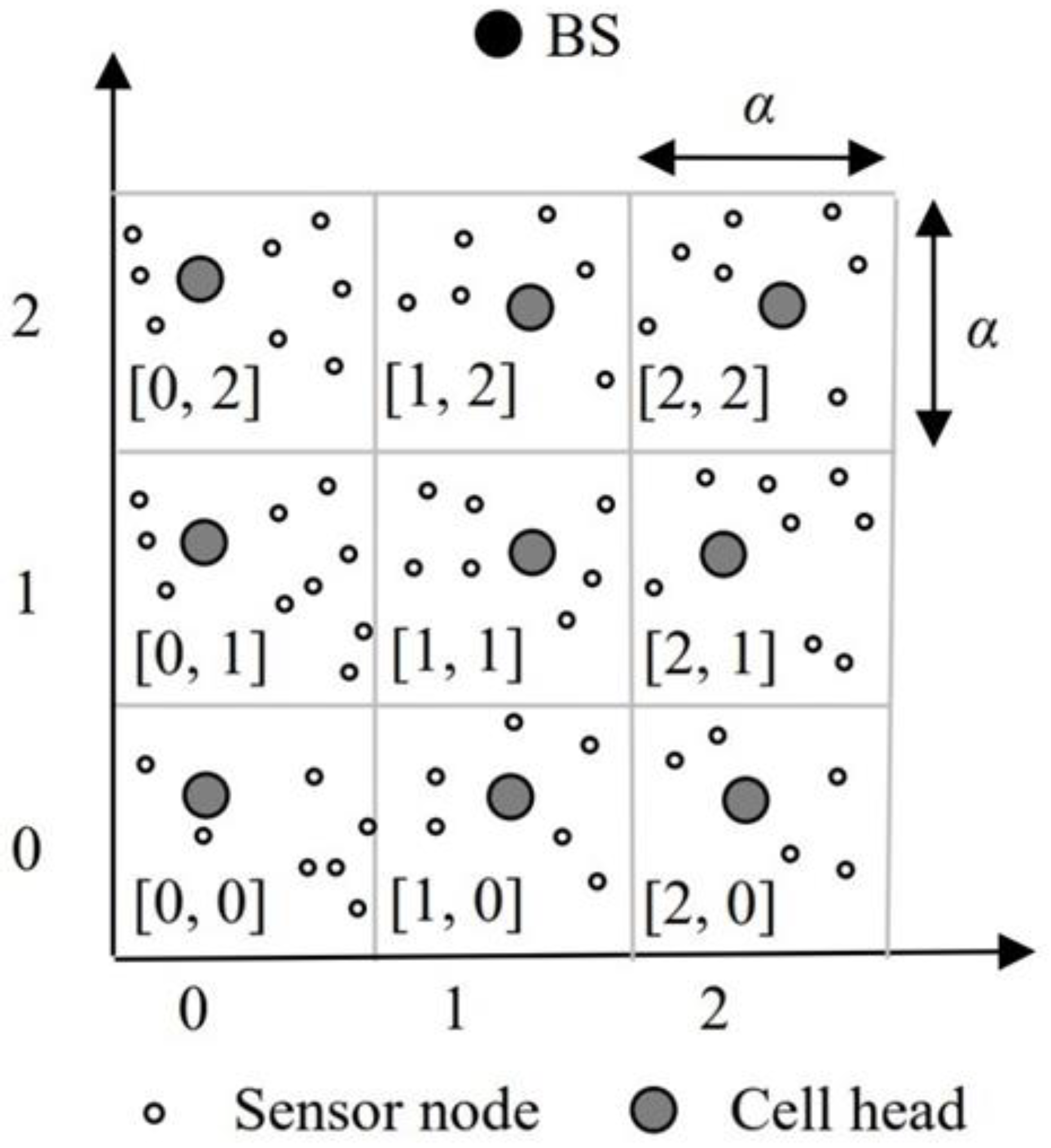
3.1. Grid Construction

This paper firstly establishes a grid infrastructure that divides the specific network area into M × N cells of a grid. Suppose the cell size is α, that is, the cell’s area is α × α. The coordinates of each cell are represented by [CX, CY]. As shown in Figure 1, we give an example where the network area is partitioned into 3 × 3 cells. The coordinates of cells, from left to right, on the first row are [0, 0], [1, 0], and [2, 0], respectively. The coordinates of cells on the second row are [0, 1], [1, 1], and [2, 1]. The coordinates of cells on the third row are [0, 2], [1, 2], and [2, 2]. The geographic location of each sensor node in the grid is represented by (x, y). Each node is equipped with a GPS device [18,19] to receive its location information. When the network lifetime begins, each sensor node calculates the coordinates of the cell that it belongs to. Next, the sensor node with the highest residual energy is elected to be the cell head in each cell. When executing each round, each cell reselects the cell head to achieve the purpose of uniform energy consumption.
Figure 1. Grid structure.

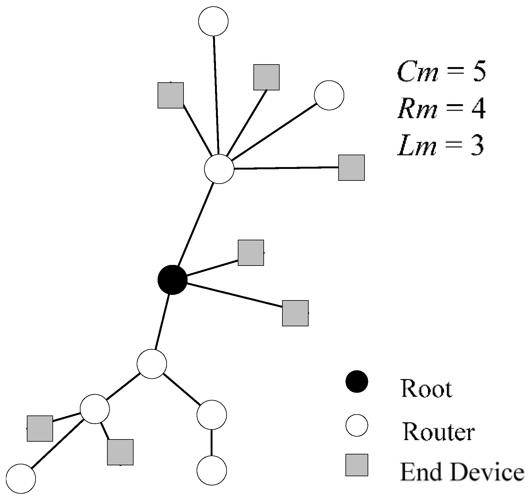
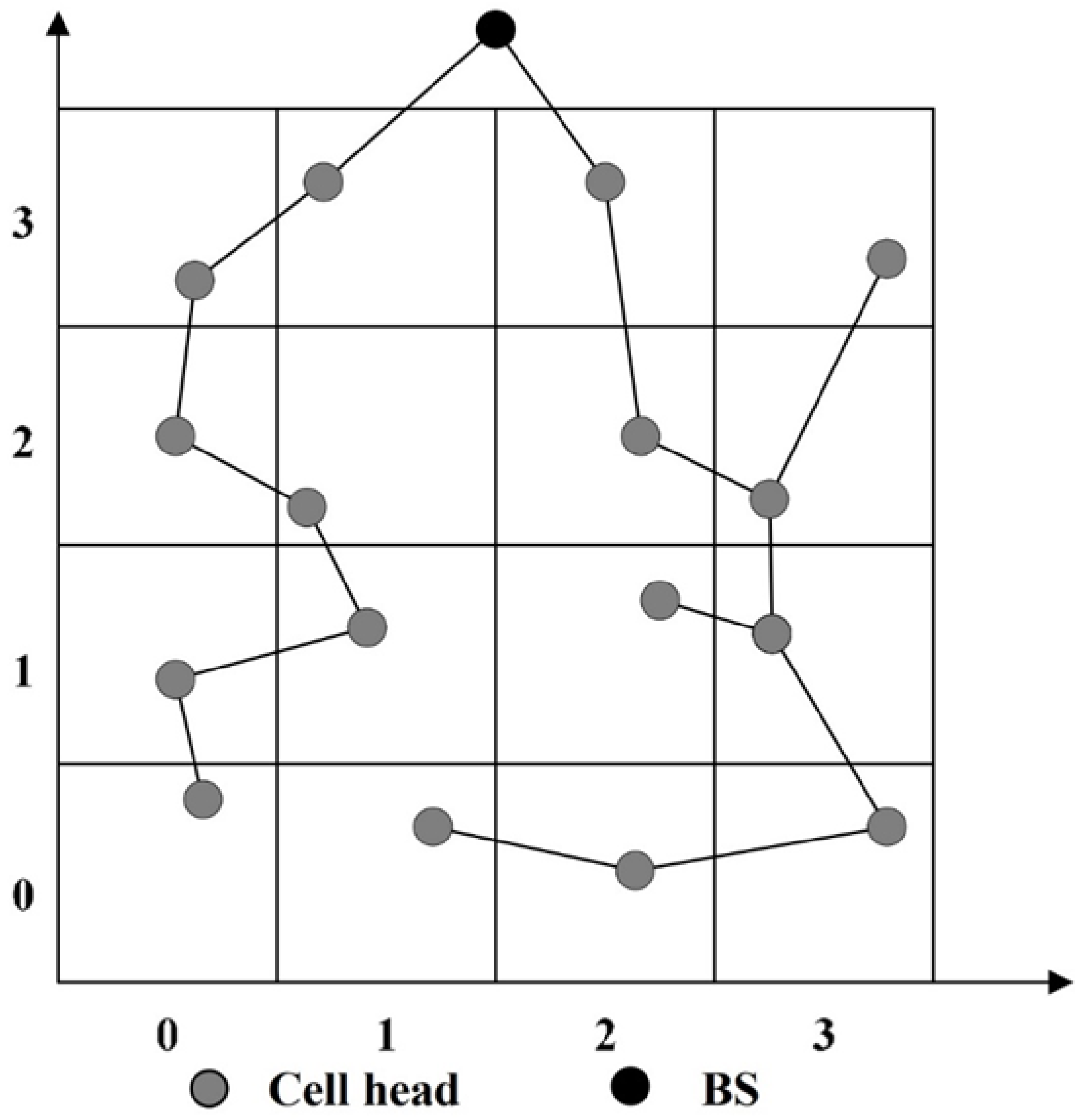
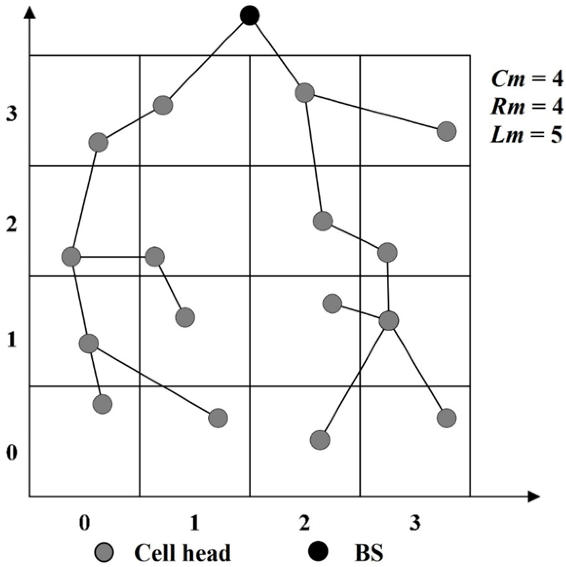
3.2. Tree Structure Construction

In the ZigBee network layer protocol [20], a distributed network address allocation algorithm is formulated to allocate network addresses to sensor nodes in WSNs. The network architecture of ZigBee is shown in Figure 2. In the network formation, the ZigBee coordinator defines the maximum number of child nodes of the router Cm, the maximum number of child routers of the router Rm, and the network depth Lm. The child nodes of the router include the other routers and the end devices, so Cm ≥ Rm. The address of each device is calculated through Cm, Rm, and Lm to calculate the relevant address parameters, thus the network addresses of the routers and the end devices can be determined [21,22].
Figure 2. Network architecture of ZigBee.
PEDAP [16] is a typical tree-based data aggregation scheme based on the minimum energy consumption spanning tree. The scheme calculates the cost of energy consumption for each node by using Equations (1) and (2) [16]. Eelec represents the power consumption for the transmitter circuit or receiver circuit, and Eamp represents the power consumption of the amplifier for data packet transmission. dij represents the distance between node i and node j, and diB represents the distance between node i and the BS. Costij(k) represents the cost for transmitting a packet k from node i to node j, and CostiB(k) represents the cost for transmitting a packet k from node i to the BS.
Costij(k) = 2 × Eelec × k + Eamp × k × dij2
CostiB(k) = Eelec × k + Eamp × k × diB2
In the tree establishment of PEDAP, the BS is responsible for serving as the root node of the tree, then the node with the minimum energy consumption is elected to join into the tree, then the process is repeated until all sensor nodes are added to the tree. In each execution round, the leaf nodes of the tree transmit the data to the upper layer of the tree according to the tree-like path for data aggregation, then the process is repeated until the data are transmitted to the BS. PEDAP can reduce the cost required for data transmission and achieve the purpose of reducing the energy consumption of sensor nodes.
This study proposes the LB-TBDAS, which is based on GB-PEDAP [17] by adding constraints on the tree structure to achieve the purpose of load balancing data transmission. In LB-TBDAS, the sensor node with the highest residual energy is elected to be the cell head in each cell. In the tree establishment of LB-TBDAS, the BS is responsible for serving as the root node of the tree, then the node (cell head) which meets the three restrictions, stated later, is elected to join the tree. Then, the nodes (cell heads) are added in sequence in the same way until all the nodes (cell heads) are added to the tree. The proposed LB-TBDAS can avoid the problems of a too long tree depth and too many child nodes (cell heads). Therefore, it can even the energy consumption of nodes to extend the network lifetime.
The node (cell head) Hi is joined into the tree, and the node (cell head) must meet the following conditions:
(a)
The node (cell head) does not exist in the tree and has the minimum energy consumption.
(b)
The current number of child nodes (cell heads) connected to the node (cell head) i is Cmi, where CmiCm.
(c)
The current depth of the node (cell head) i is Lmi, where LmiLm.
In general, the location of the BS will affect the topology of the tree structure, which will also affect the network depth Lm. The network depth Lm can be determined using Equation (3).
L m = M + N 4
In the following, we give an example to discuss the differences between the tree structure of GB-PEDAP and that of the proposed LB-TBDAS. We assume that the BS is located above the sensing area. The tree-like path establishment of GB-PEDAP and LB-TBDAS is shown in Figure 3 and Figure 4, respectively. In Figure 3, the depths of the leaf nodes of the GB-PEDAP tree structure are 7, 7, 5, and 4, respectively, and Lm = max (7, 7, 5, 4) = 7. In Figure 4, the depths of the leaf nodes of the LB-TBDAS tree structure are 5, 5, 5, 5, 5, 5, and 2, respectively, and Lm = max (5, 5, 5, 5, 5, 5, 2) = 5. Compared with the GB-PEDAP tree structure, the depth of the LB-TBDAS tree structure is more average. Since LB-TBDAS limits the network depth of the tree structure, the number of hops for data transmission is reduced, thus reducing the energy consumption of sensor nodes. In addition, we use the constraint of Cm, so that the number of child nodes connected by a node will not be too many, thereby avoiding the problem of hotspots. The tree-like path establishment algorithm of LB-TBDAS is shown in Algorithm 1.
Algorithm 1: The tree-like path establishment algorithm of LB-TBDAS.
Step 1: System initialization
(1) Sensor nodes are randomly deployed in the specific network area.
(2) The network area is partitioned into M × N cells of a grid.
(3) The sensor node with the highest residual energy is elected to be the cell head in each cell.
Step 2: Tree initialization
(1) The BS is responsible for serving as the root node.
(2) The network depth is Lm and the maximum number of child nodes (cell heads) is Cm.
Step 3: Tree construction
Figure 3. Tree-like path establishment of GB-PEDAP.
Figure 4. Tree-like path establishment of TBDAS.

3.3. Data Transmission

When the tree structure is established, the sensing data of sensor nodes are collected and transmitted to their cell head in each cell, and then the sensing data are transmitted to the BS through the tree-like path. For the next execution round, the cell head is re-selected and the tree is re-established; it is processed in the same way. The data aggregation scheme can evenly consume energy, thereby prolonging the network lifetime.

4. Simulation Results

In this study, we developed a simulator with MATLAB software. In the simulations, the energy consumption of the sensor nodes in the sensing network adopts the First Order Radio Model [23,24]. When a sensor node does not have enough residual energy for data transmission, the sensor node will be marked as a dead node and the node will no longer transmit data. The network size is 100 m × 100 m and the location of BS is (50, 150). The number of cells is assumed to be 10 × 10 and the initial energy is assumed to be 0.25 J/node. The number of nodes is from 100 to 400 and the packet size is 512 bits. The network depth (Lm) ranges from 5 to 10 and the maximum number of child nodes (Cm) can be 4 and 7, respectively. Eelec is 50 nJ/bit and Eamp is 100 pJ/bit/m2. The simulation parameters of this study are shown in Table 1.
Table 1. Simulation parameters.

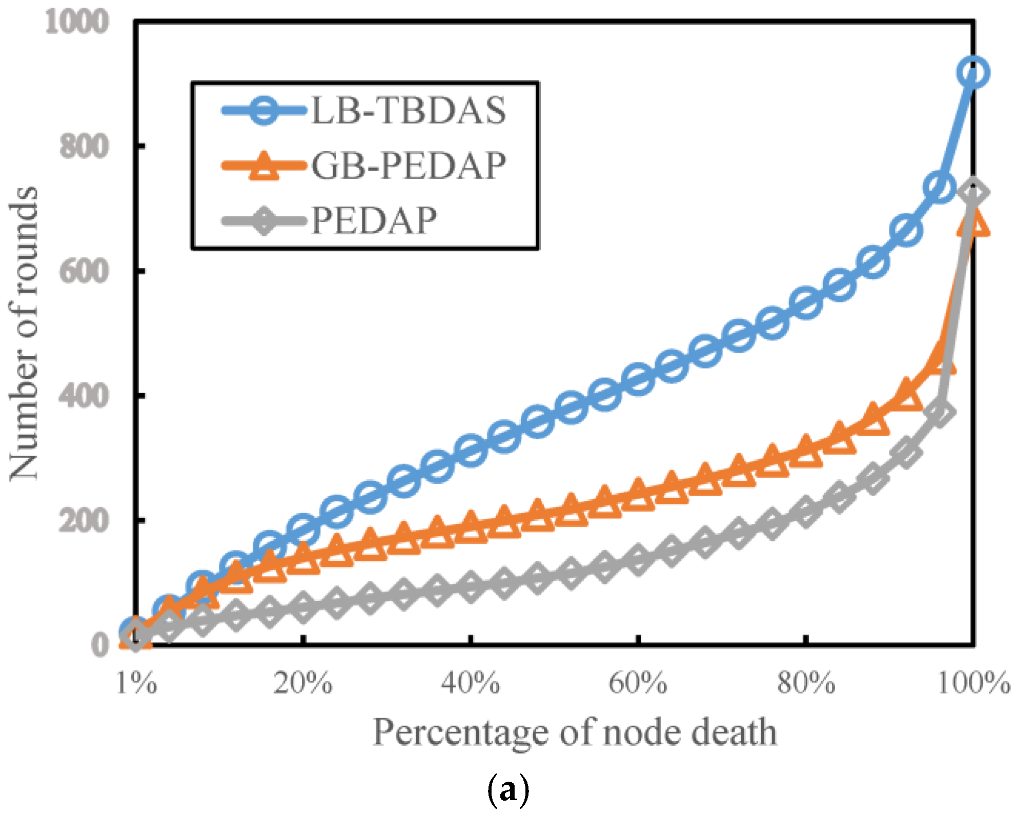
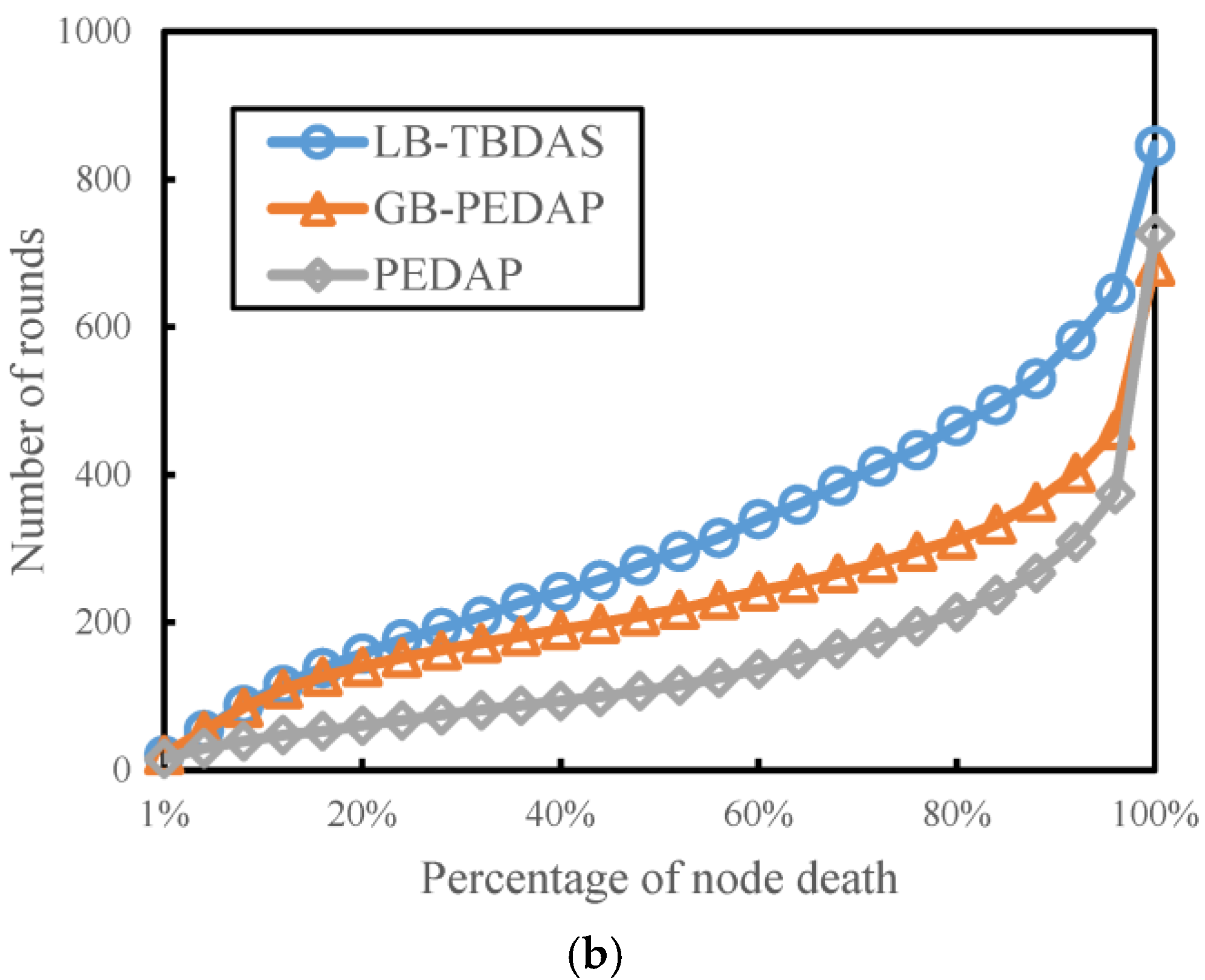
4.1. Number of Rounds Versus Node Death Percentages

We study the number of execution rounds of the three schemes at different node death percentages and explore the effect of the LB-TBDAS network depth Lm. The number of cells is assumed to be 10 × 10 and the number of nodes is 300. The network depths (Lm) are 5 and 10, respectively. The maximum number of child nodes (Cm) is 4. We simulated PEDAP, GB-PEDAP, and LB-TBDAS to observe the execution rounds of different node death percentages. In Figure 5a,b, when the node death percentage increases, the number of execution rounds of various schemes also increases. In addition, the LB-TBDAS network depth Lm is smaller, and there will be more execution rounds. Overall, the number of execution rounds of LB-TBDAS is better than GB-PEDAP and PEDAP. This is because LB-TBDAS limits the width and depth of the tree-like path structure, which can uniformize the energy consumption of nodes.
Figure 5. Number of rounds versus node death percentages: (a) Lm = 5; (b) Lm = 10.

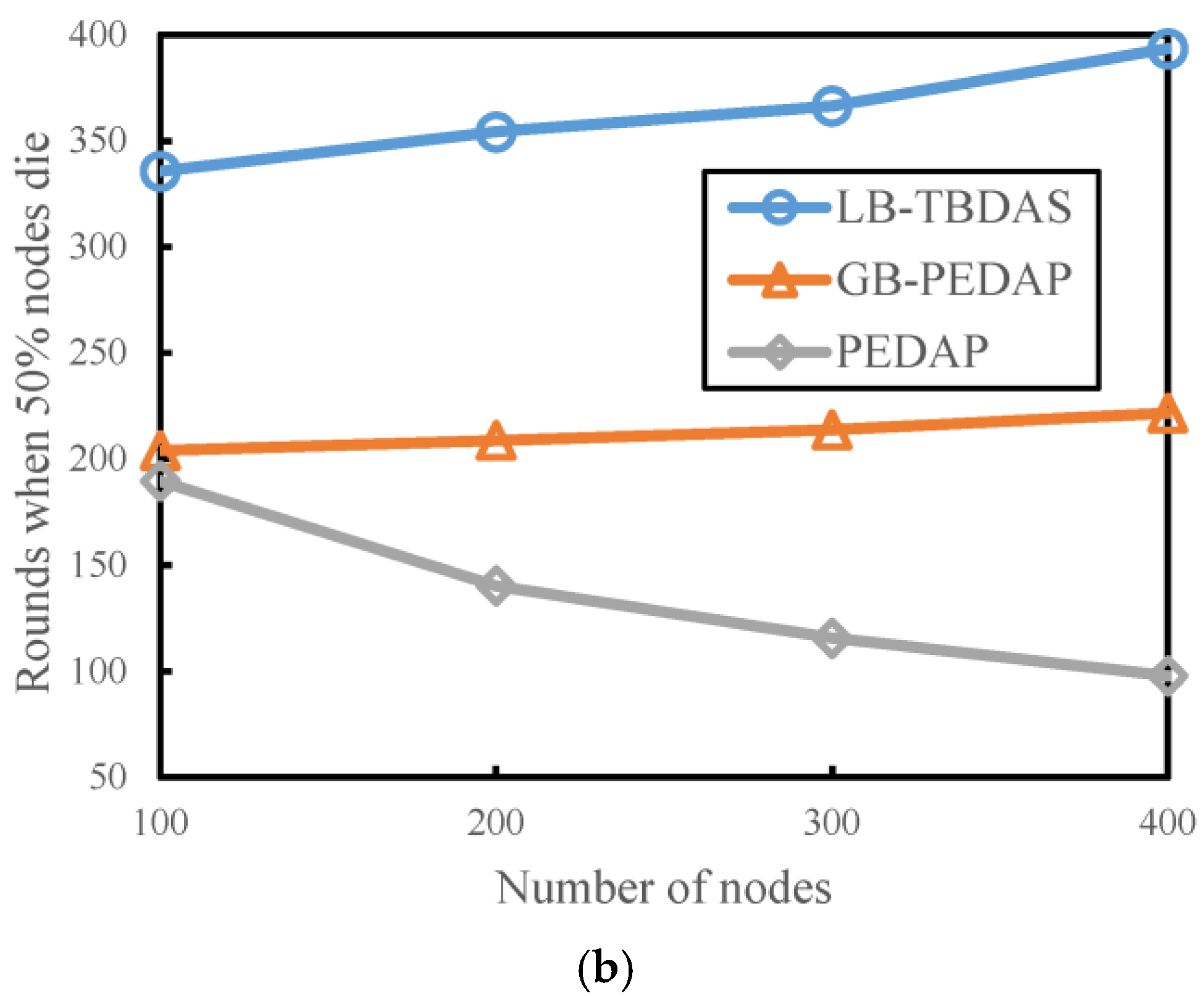
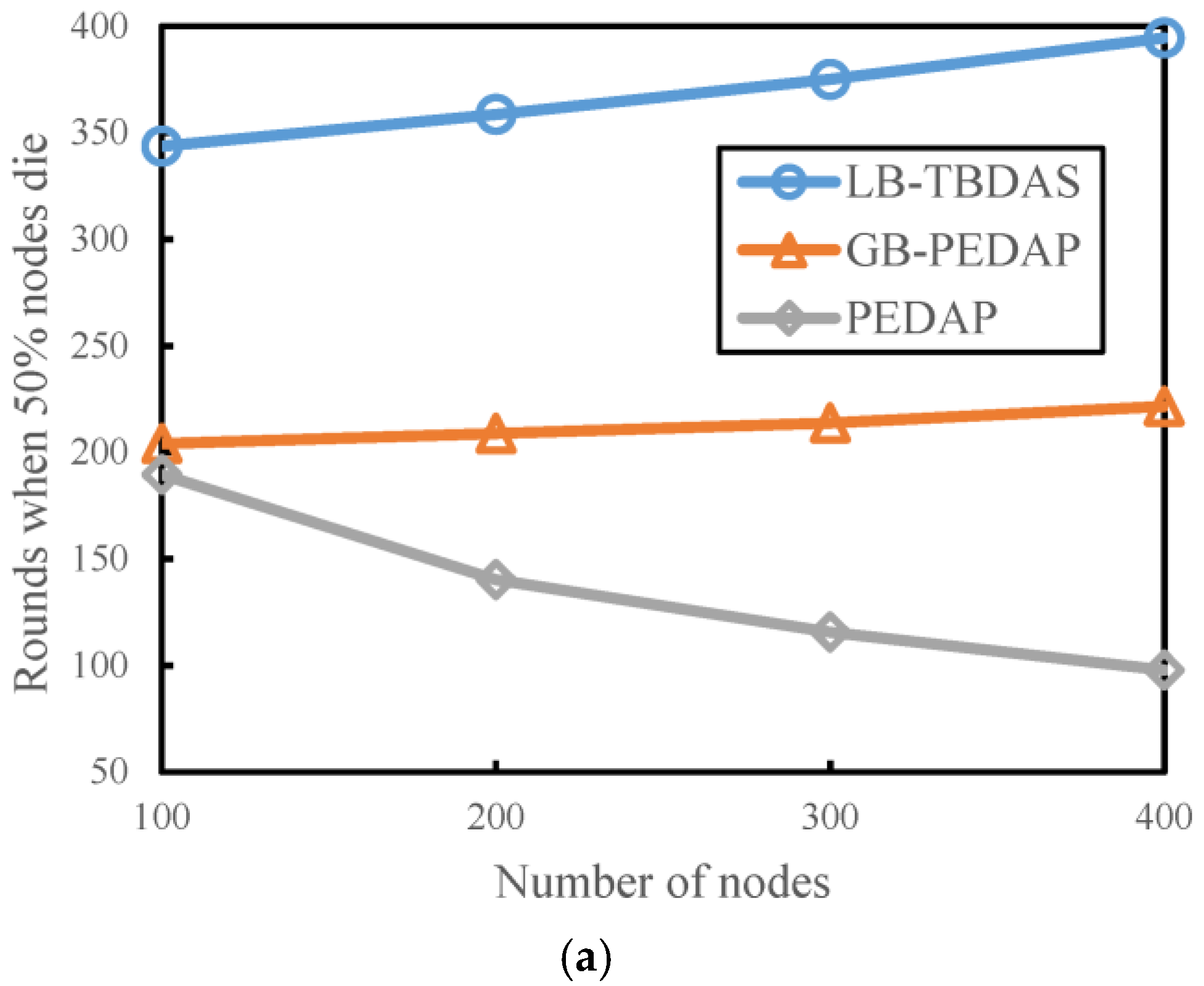
4.2. Number of Rounds when 50% of Nodes Die versus Number of Nodes

We observe the number of execution rounds of each scheme when 50% of the nodes die with different numbers of nodes and explore the impact of different values of the maximum number of child nodes (Cm) for LB-TBDAS. The number of cells is assumed to be 10 × 10 and the number of nodes is assumed to be 300. The network depth (Lm) is 5. The maximum number of child nodes (Cm) can be 4 and 7, respectively. In Figure 6a,b, when the number of nodes gradually increases, the execution rounds of LB-TBDAS and GB-PEDAP also increase when 50% of the nodes die, but the execution rounds of PEDAP decrease when 50% of the nodes die. With the same number of nodes, LB-TBDAS executes more rounds than GB-PEDAP and PEDAP when 50% of the nodes die. In LB-TBDAS, as the maximum number of child nodes Cm increases, the number of execution rounds increases slightly. When the maximum number of child nodes is larger, the number of hops for data transmission decreases, resulting in a more even load of node energy consumption.
Figure 6. Number of rounds when 50% of nodes die versus number of nodes: (a) Cm = 4; (b) Cm = 7.

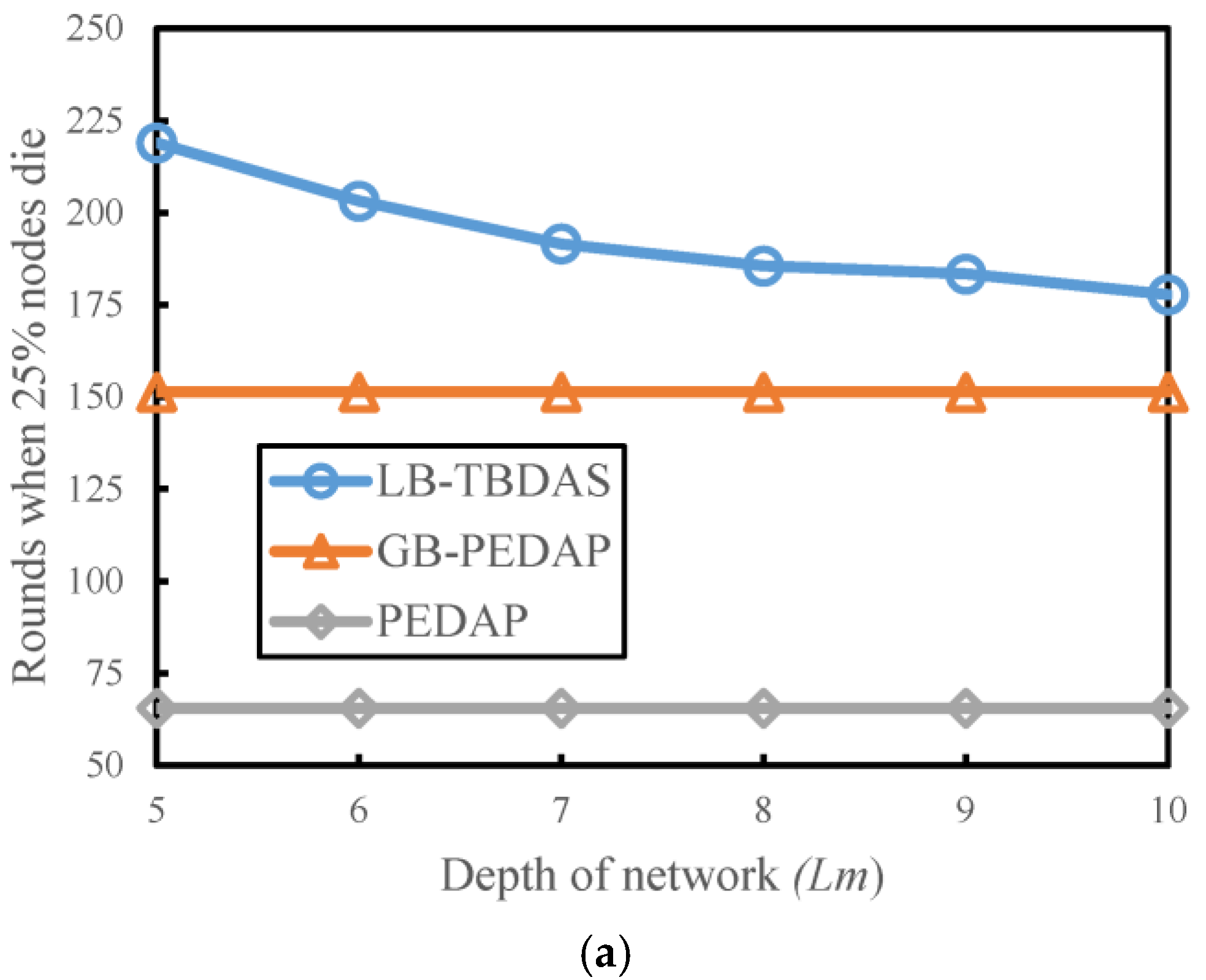
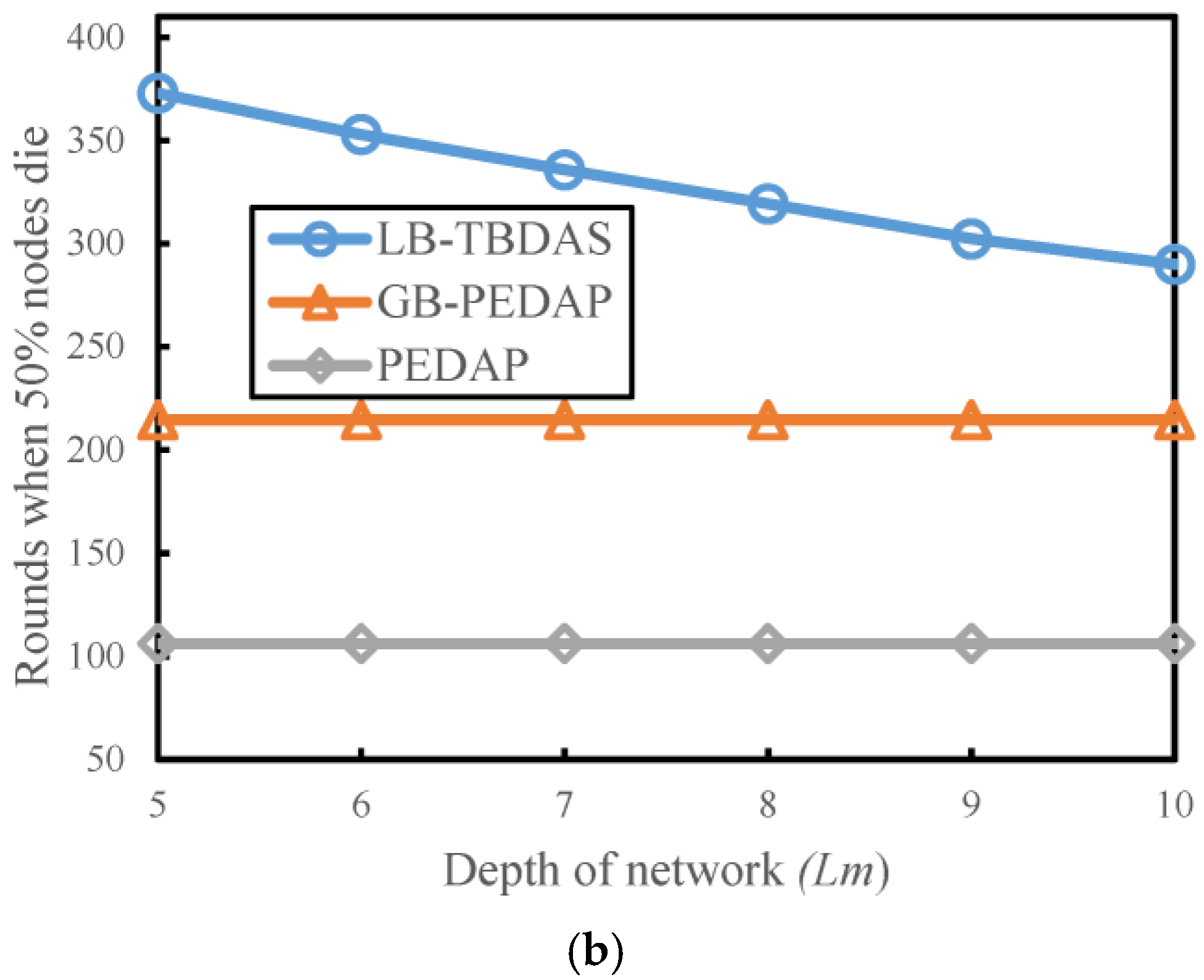
4.3. Number of Rounds Versus Depth of Network

We explore the number of execution rounds of each scheme when 25% and 50% of nodes die at different network depths Lm. The number of cells is assumed to be 10 × 10 and the number of nodes is assumed to be 300. The network depth (Lm) is from 5 to 10. The maximum number of child nodes (Cm) is 4. In Figure 7a,b, when the network depth Lm increases, the number of execution rounds of LB-TBDAS at the 25% and 50% node death percentages also increases. As the network depth of LB-TBDAS increases, the number of execution rounds decreases. When the network depth is deeper, the number of hops for data transmission increases, resulting in a more uneven load of node energy consumption.
Figure 7. Number of rounds versus depth of network: (a) 25% of nodes die; (b) 50% of nodes die.

4.4. Total Consumed Energy versus Number of Rounds

We study the total energy consumption for sensor nodes in the WSN. The total energy consumption is mainly to observe the energy consumption generated when each node transmits and receives data in each round. The number of cells is assumed to be 10 × 10, the number of nodes is assumed to be 300, and the initial energy is assumed to be 0.25 J. As shown in Figure 8, when the number of execution rounds is gradually increased, the total energy consumption will also increase. The total energy consumption of LB-TBDAS was significantly less than that of GB-PEDAP and PEDAP. This is because a factor considering energy consumption is added to the tree-like path structure of LB-TBDAS, which can reduce the energy consumption of nodes.
Figure 8. Total consumed energy versus number of rounds.

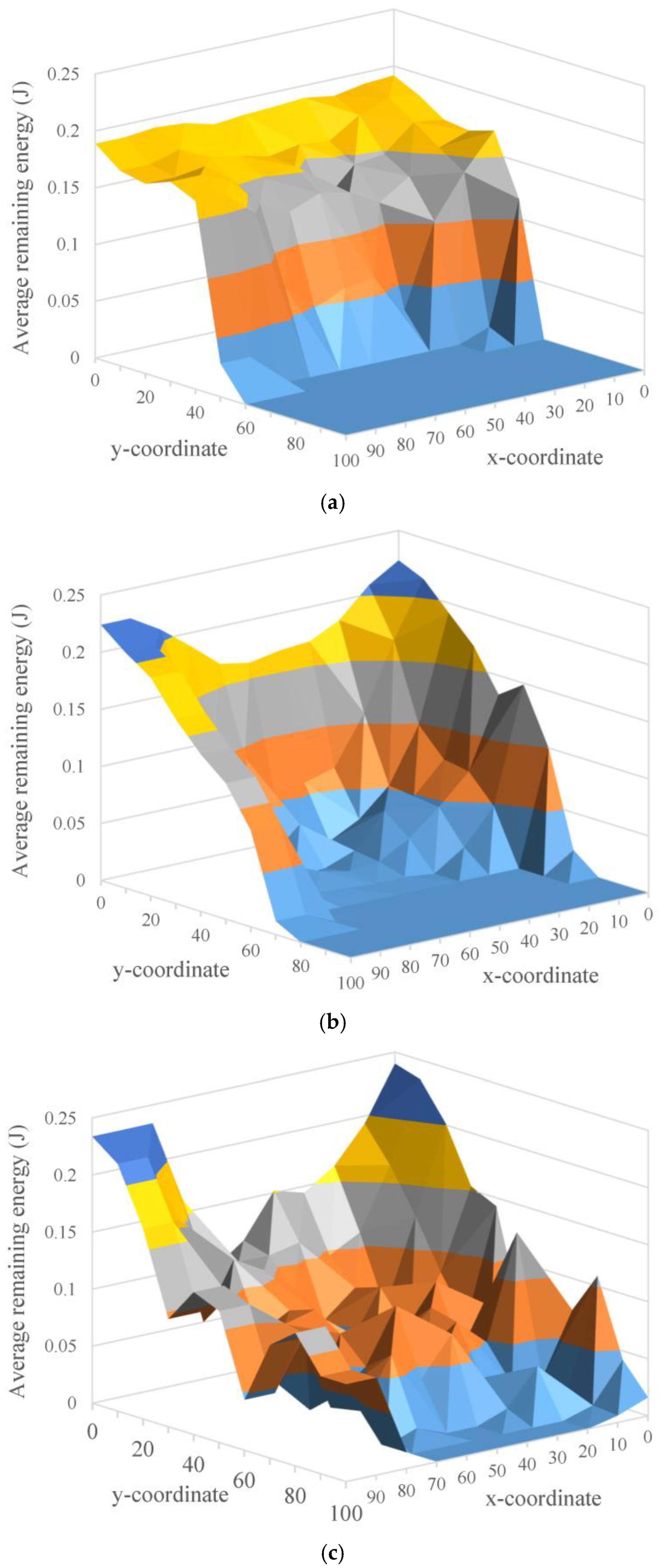
4.5. Energy Distribution for Sensor Nodes

We discuss the energy distribution for sensor nodes in the WSN. We simulate the residual energy distribution of nodes in the sensing area when 50% of the sensor nodes die. In Figure 9a–c, when half of the nodes die, the energy distribution of LB-TBDAS nodes is relatively uniform, and the remaining energy is relatively large; the energy of nodes in the middle area of GB-PEDAP is particularly low and relatively uneven; and PEDAP is completely unevenly distributed in the entire sensing area. This is because LB-TBDAS has the characteristic of load balancing, which can make the energy distribution of nodes more even.
Figure 9. Energy distribution for sensing nodes: (a) LB-TBDAS; (b) GB-PEDAP; (c) PEDAP.
The comparisons of LB-TBDAS, GB-PEDAP, and PEDAP are shown in Table 2. The hierarchical architecture of LB-TBDAS and GB-PEDAP includes two layers and that of PEDAP is a single layer. The data transmission of LB-TBDAS and GB-PEDAP includes direct transmission and tree-path transmission, while the data transmission of PEDAP is tree-path transmission. The energy consumption types of LB-TBDAS, GB-PEDAP, and PEDAP are load balancing, uniform, and general, respectively. The energy efficiency of LB-TBDAS is the best.
Table 2. The comparisons of LB-TBDAS, GB-PEDAP, and PEDAP.
In PEDAP, the tree construction does not consider the residual energy of the current sensor nodes, which makes the residual energy distribution very uneven. The GB-PEDAP is a two-layer architecture which builds a grid structure in the sensing area, and then uses Prim’s algorithm to construct an energy consumption uniform tree for data aggregation. The residual energy distribution of GB-PEDAP is more uniform than that of PEDAP. The proposed LB-TBDAS is also a two-layer architecture with a grid which constructs an energy consumption load balancing tree for data aggregation. The residual energy distribution of LB-TBDAS is more even than that of GB-PEDAP and PEDAP.

5. Conclusions

In this study, we propose an energy-efficient load balancing tree-based data aggregation scheme (LB-TBDAS) with a grid-based WSN. This scheme uses the minimum spanning tree algorithm to build the tree structure in the grid-based WSN. The proposed LB-TBDAS uses three constraints to construct a tree-like data transmission path with load balancing, and the energy load can be evenly dispersed. Simulation results show that the average remaining energy of LB-TBDAS is significantly better than that of GB-PEDAP and PEDAP. The proposed LB-TBDAS extends over 100% of the network lifetime compared to GB-PEDAP and PEDAP. The proposed LB-TBDAS can effectively reduce the energy consumption of sensor nodes, thereby prolonging the network lifetime.

Author Contributions

Conceptualization, N.-C.W.; methodology, N.-C.W., C.-Y.L. and Z.-Z.C.; software, Y.-L.C. and Z.-Z.C.; validation, Y.-L.C. and C.-M.C.; formal analysis, N.-C.W. and C.-Y.L.; Investigation, C.-Y.L. and Z.-Z.C.; resources, C.-Y.L., Y.-L.C. and C.-M.C.; data curation, Y.-L.C. and C.-M.C.; writing—original draft preparation, C.-M.C. and Z.-Z.C.; writing—review and editing, N.-C.W. and C.-M.C.; Visualization, C.-Y.L. and Y.-L.C.; supervision, N.-C.W.; project administration, N.-C.W.; funding acquisition, N.-C.W. and C.-Y.L. All authors have read and agreed to the published version of the manuscript.

Funding

This work was supported by the Ministry of Science and Technology of the Republic of China under grant MOST-110-2221-E-239-002.

Institutional Review Board Statement

Not applicable.

Data Availability Statement

Not applicable.

Conflicts of Interest

The authors declare no conflict of interest.

References

  1. Ramson, S.R.J.; Moni, D.J. Applications of Wireless Sensor Networks—A Survey. In Proceedings of the International Conference on Innovations in Electrical, Electronics, Instrumentation and Media Technology, Coimbatore, India, 3–4 February 2017; pp. 325–329. [Google Scholar]
  2. Sharma, S.; Kaur, A. Survey on Wireless Sensor Network, Its Applications and Issues. J. Phys. Conf. Ser. 2021, 1969, 1–10. [Google Scholar] [CrossRef]
  3. Wang, X.; Chen, H. A Survey of Compressive Data Gathering in WSNs for IoTs. Wirel. Commun. Mob. Comput. 2022, 2022, 1–14. [Google Scholar] [CrossRef]
  4. Hilmani, A.; Maizate, A.; Hassouni, L. Automated Real-Time Intelligent Traffic Control System for Smart Cities using Wireless Sensor Networks. Wirel. Commun. Mob. Comput. 2020, 2020, 1–28. [Google Scholar] [CrossRef]
  5. Durai, S.K.S.; Duraisamy, B.; Thirukrishna, J.T. Certain Investigation on Healthcare Monitoring for Enhancing Data Transmission in WSN. Int. J. Wirel. Inf. Netw. 2021, 1–8. [Google Scholar]
  6. Majid, M.; Habib, S.; Javed, A.R.; Rizwan, M.; Srivastava, G.; Gadekallu, T.R.; Lin, C.-W. Applications of Wireless Sensor Networks and Internet of Things Frameworks in the Industry Revolution 4.0: A Systematic Literature Review. Sensors 2022, 22, 2087. [Google Scholar] [CrossRef] [PubMed]
  7. Braginsky, D.; Estrin, D. Rumor Routing Algorithm for Sensor Network. In Proceedings of the 1st ACM International Workshop on Wireless Sensor Networks and Applications, Atlanta, GA, USA, 28 September 2002; pp. 22–31. [Google Scholar]
  8. Lindsey, S.; Raghavendra, C.S. PEGASIS: Power-Efficient Gathering in Sensor Information System. In Proceedings of the IEEE Aerospace Conference, Big Sky, MT, USA, 9–16 March 2002; Volume 3, pp. 1125–1130. [Google Scholar]
  9. Jung, S.M.; Han, Y.J.; Chung, T.M. The Concentric Clustering Scheme for Efficient Energy Consumption in the PEGASIS. In Proceedings of the 9th International Conference on Advanced Communication Technology, Phoenix Park, Korea, 12–14 February 2007; Volume 1, pp. 260–265. [Google Scholar]
  10. Ye, F.; Haiyun, L.; Jerry, C.; Songwu, L.; Zhang, L. A Two-Tier Data Dissemination Model for Large-Scale Wireless Sensor Networks. In Proceedings of the ACM International Conference on Mobile Computing and Networking, London, UK, 21–25 September 2002; pp. 148–159. [Google Scholar]
  11. Nagesh, R.; Raga, S.; Mishra, S. Elimination of Redundant Data to Enhance Wireless Sensor Network Performance Using Multi Level Data Aggregation Technique. In Proceedings of the 2019 International Conference on Computing, Communication and Networking Technologies, Kanpur, India, 6–8 July 2019; pp. 1–5. [Google Scholar]
  12. Deepakraj, D.; Raja, K. Hybrid Data Aggregation Algorithm for Energy Efficient Wireless Sensor Networks. In Proceedings of the 2021 International Conference on Intelligent Communication Technologies and Virtual Mobile Networks, Tirunelveli, India, 4–6 February 2021; pp. 7–12. [Google Scholar]
  13. Lee, W.M.; Wong, V.W.S. E-Span and LPT for Data Aggregation in Wireless Sensor Networks. In Proceedings of the Computer Communications, Arlington, VA, USA, 9–11 October 2006; Volume 29, pp. 2506–2520. [Google Scholar]
  14. Bandral, M.S.; Jain, S. Energy Efficient Protocol for Wireless Sensor Network. In Proceedings of the Recent Advances and Innovations in Engineering, Jaipur, India, 9–11 May 2014; pp. 477–482. [Google Scholar]
  15. Zhou, L.; Ge, C.; Hu, S.; Su, C. Energy-Efficient and Privacy-Preserving Data Aggregation Algorithm for Wireless Sensor Networks. IEEE Internet Things J. 2020, 7, 3948–3957. [Google Scholar] [CrossRef]
  16. Tan, H.O.; Korpeoglu, I. Power Efficient Data Gathering and Aggregation in Wireless Sensor Networks. ACM SIGMOD Rec. 2003, 32, 66–71. [Google Scholar] [CrossRef]
  17. Wang, N.-C.; Chen, Y.-L.; Huang, Y.-F.; Chen, C.-M.; Lin, W.-C.; Lee, C.-Y. An Energy Aware Grid-Based Clustering Power Efficient Data Aggregation Protocol for Wireless Sensor Networks. Appl. Sci. 2022, 12, 1. [Google Scholar] [CrossRef]
  18. Albowitz, J.; Chen, A.; Shang, L. Recursive Position Estimation in Sensor Networks. In Proceedings of the International Conference on Network Protocols, Riverside, CA, USA, 11–14 November 2001; pp. 35–41. [Google Scholar]
  19. Kaplan, E.D. Understanding GPS: Principles and Applications; Artech Hourse: Boston, MA, USA, 1996. [Google Scholar]
  20. Pan, M.-S.; Tseng, Y.-C. The Orphan Problem in ZigBee-Based Wireless Sensor Networks. In Proceedings of the Tenth ACM Symposium on Modeling, Analysis, and Simulation of Wireless and Mobile Systems, Crete Island, Greece, 22–26 October 2007; pp. 95–98. [Google Scholar]
  21. ZigBee Alliance. ZigBee Specification, Version 1.0; ZigBee Alliance: Davis, CA, USA, 2004. [Google Scholar]
  22. ZigBee Alliance. ZigBee—2007 Specification; ZigBee Alliance: Davis, CA, USA, 2007. [Google Scholar]
  23. Heinzelman, W.R.; Chandrakasan, A.; Balakrishnan, H. Energy-Efficient Communication Protocol for Wireless Microsensor Networks. In Proceedings of the IEEE Annual Hawaii International Conference on Systems Sciences, Maui, HI, USA, 6 January 2000; pp. 3005–3014. [Google Scholar]
  24. Andreou, P.; Pamboris, A.; Zeinalipour-Yazti, D.; Chrysanthis, P.K.; Samaras, G. ETC: Energy-Driven Tree Construction in Wireless Sensor Networks. In Proceedings of the International Conference on Mobile Data Management: Systems, Services and Middleware, Taipei, Taiwan, 18–20 May 2009; pp. 35–40. [Google Scholar]
Publisher’s Note: MDPI stays neutral with regard to jurisdictional claims in published maps and institutional affiliations.

Article Metrics

Citations

Article Access Statistics

Multiple requests from the same IP address are counted as one view.