
Ship Berthing and Unberthing Monitoring System in the Ferry Terminal

Abstract
1. Introduction
2. Materials and Methods
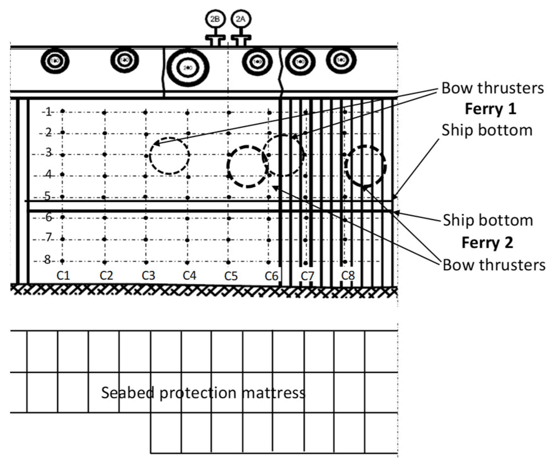
2.1. Measurement of Bow Thruster-Generated Pressure on the Quay Wall
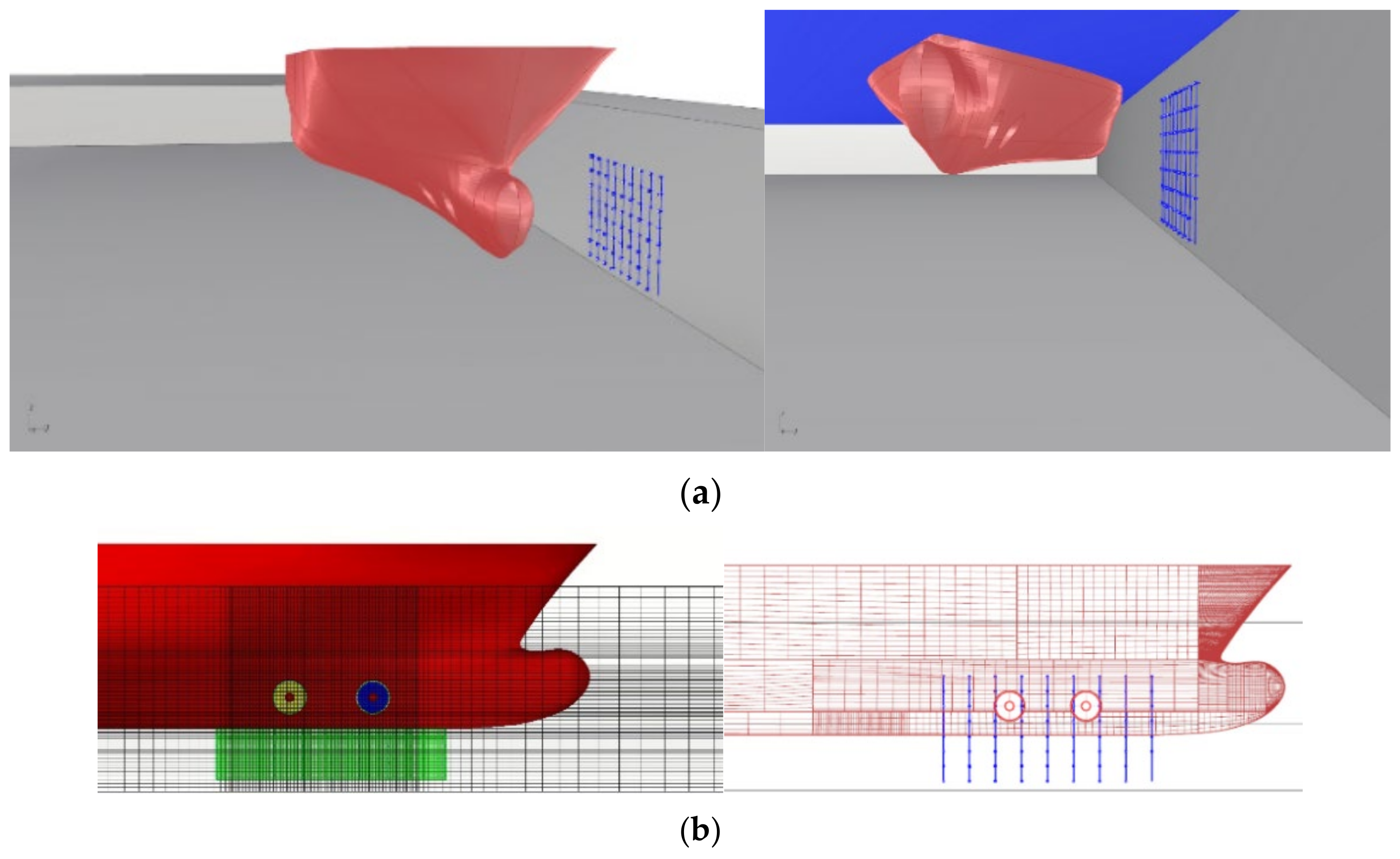
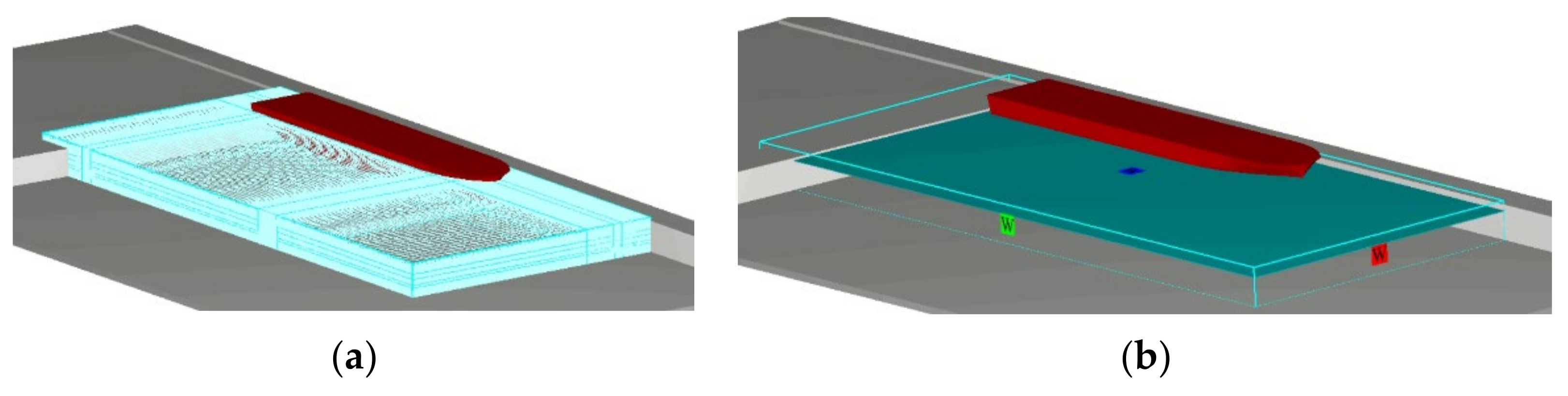
2.2. CFD Simulation
3. Results and Discussion
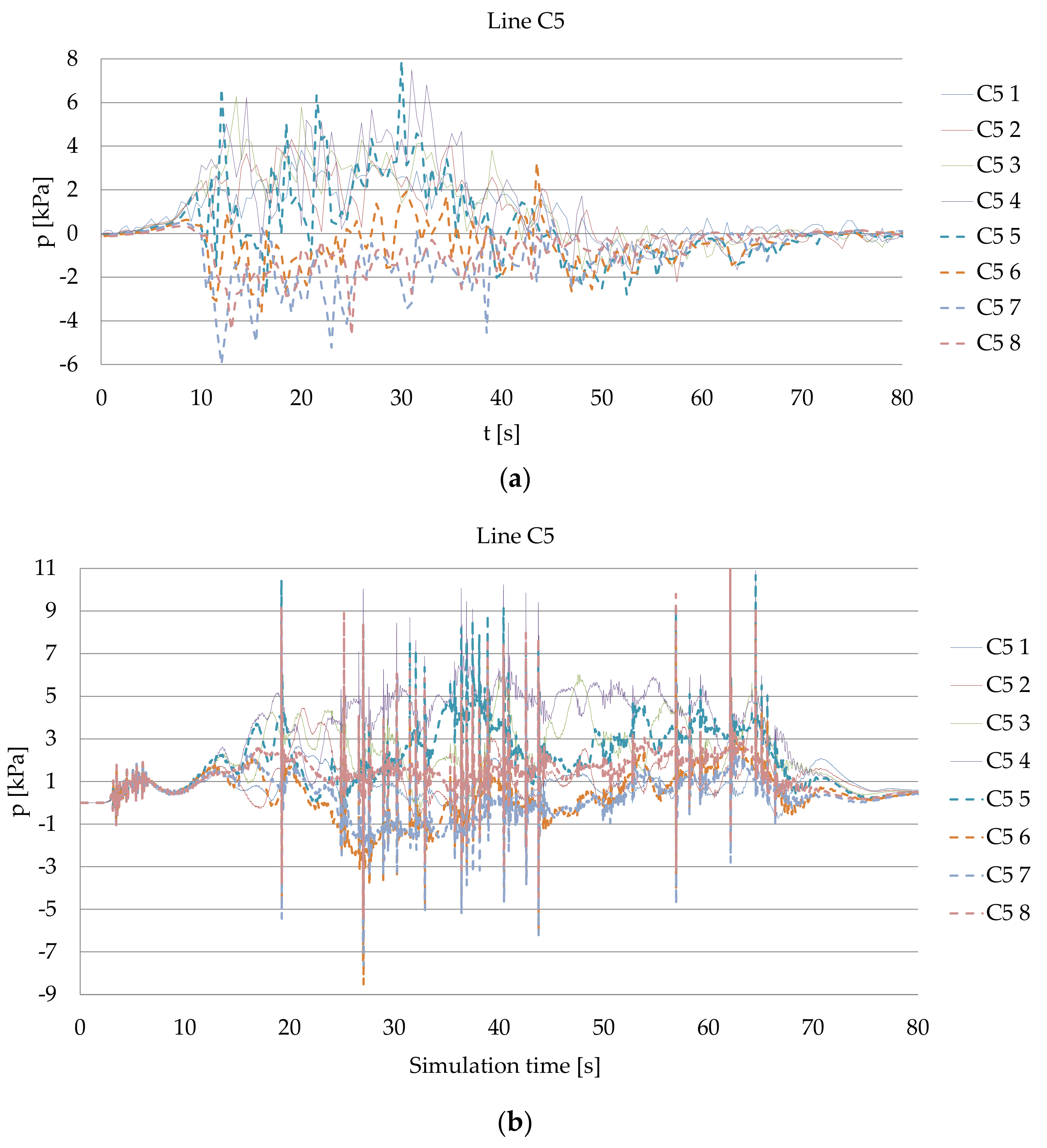
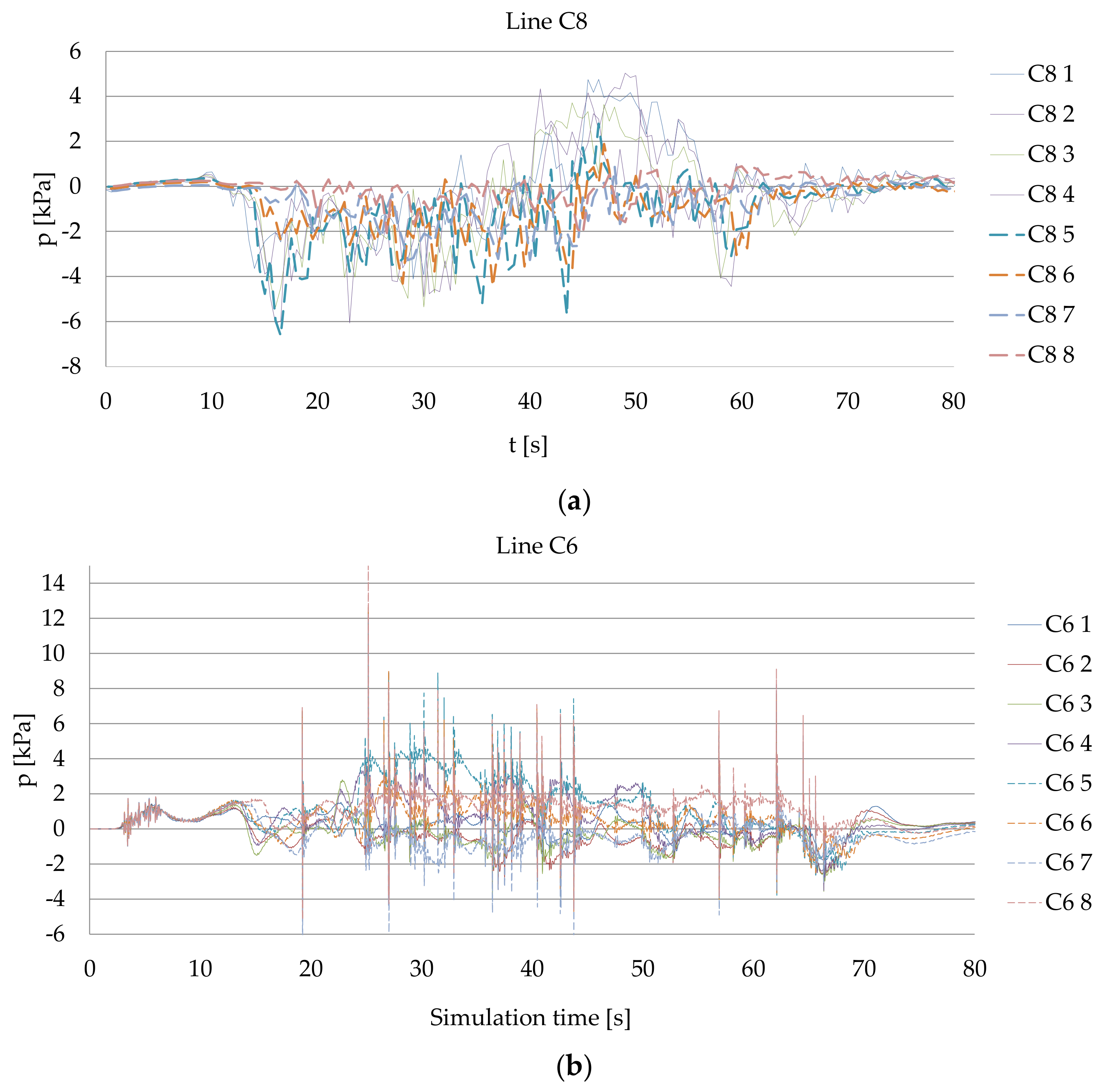
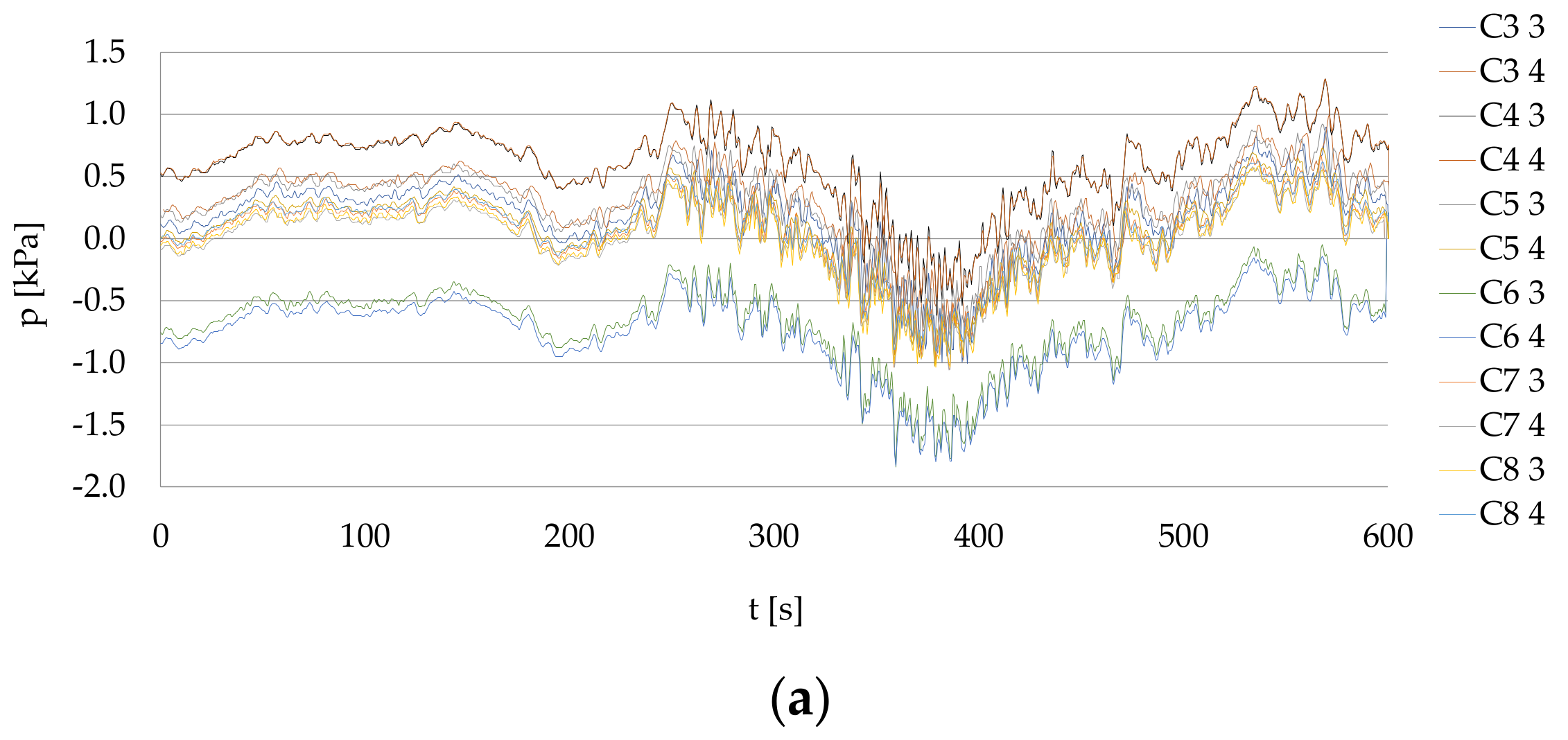
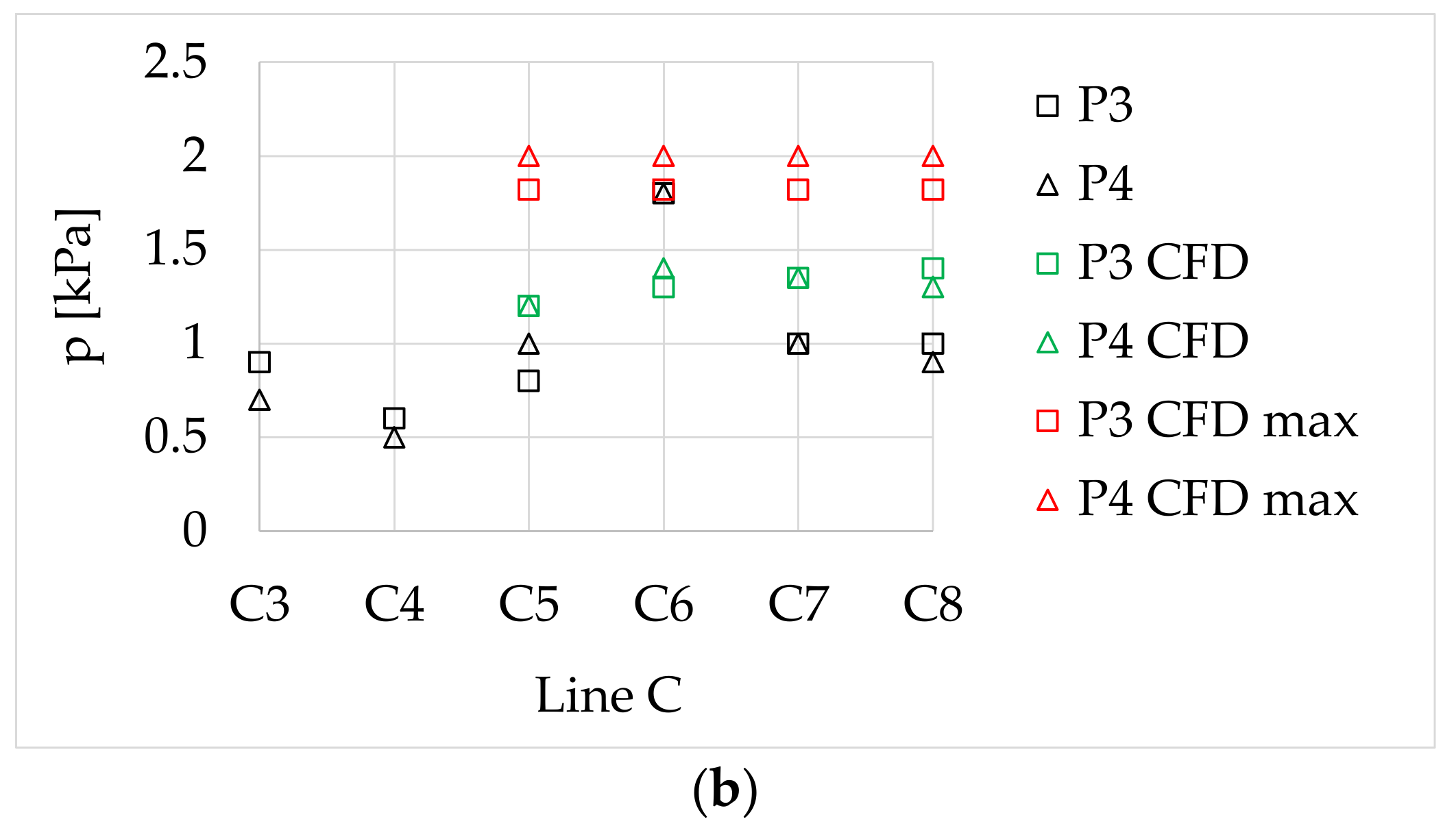
3.1. Bow Thruster Generated Pressure on the Quay Wall
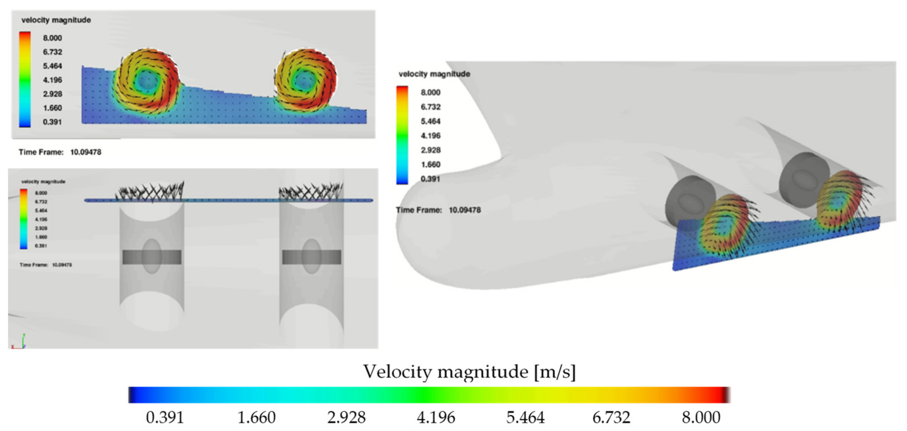
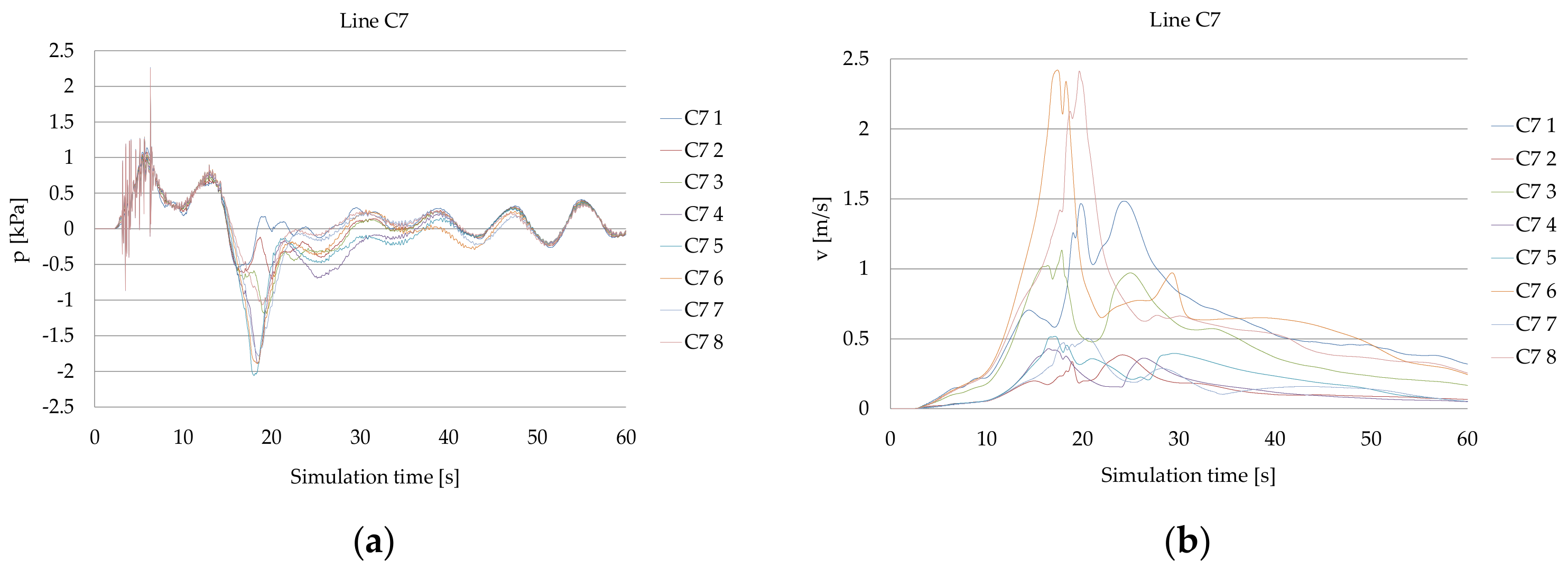
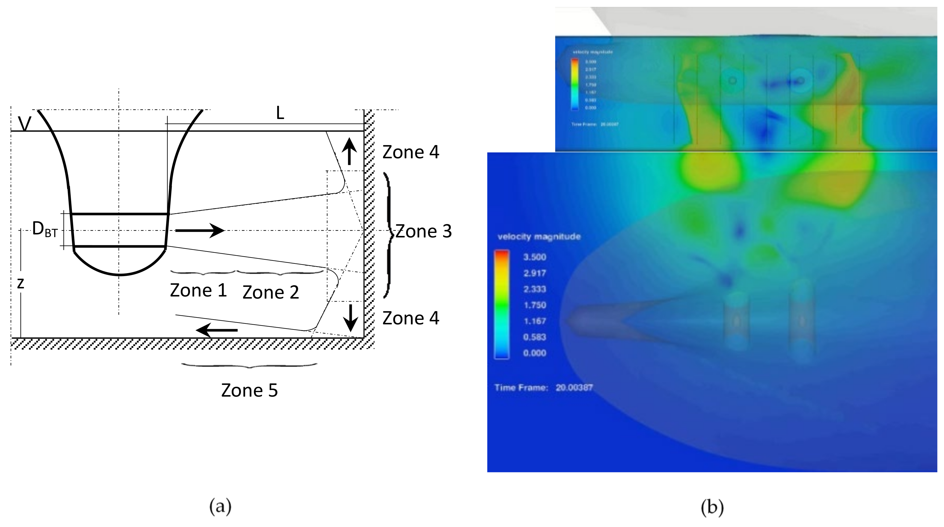
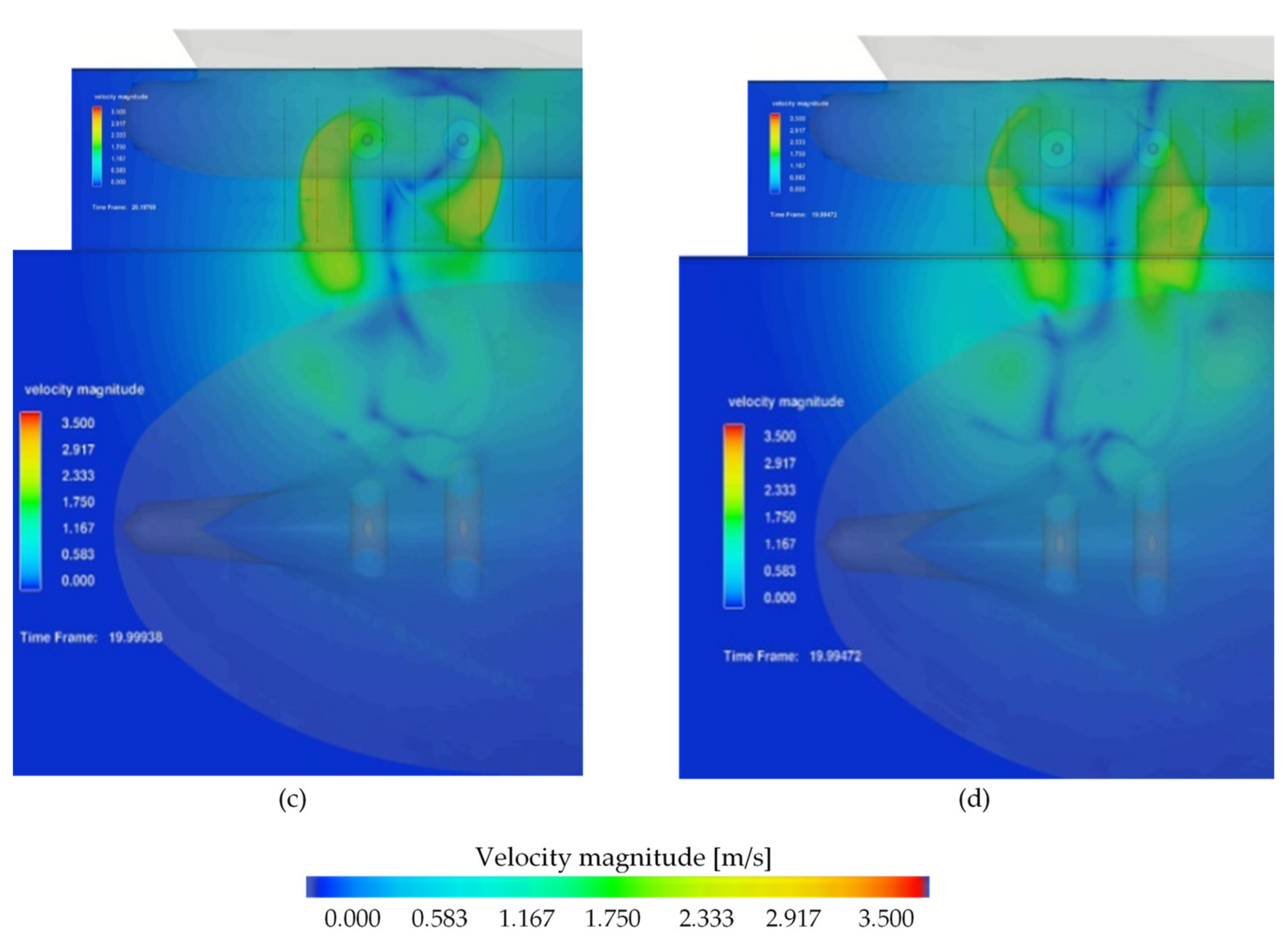
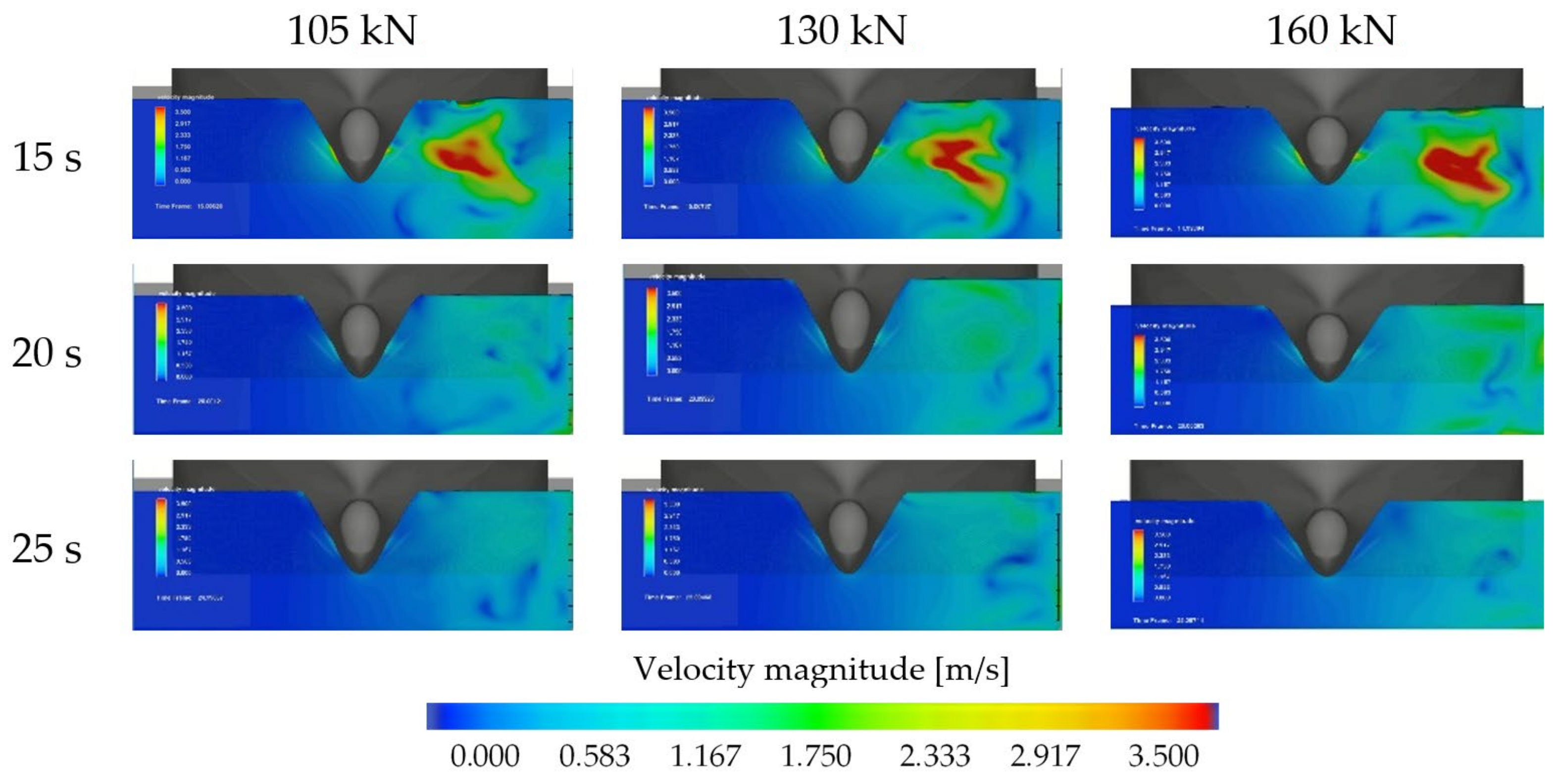
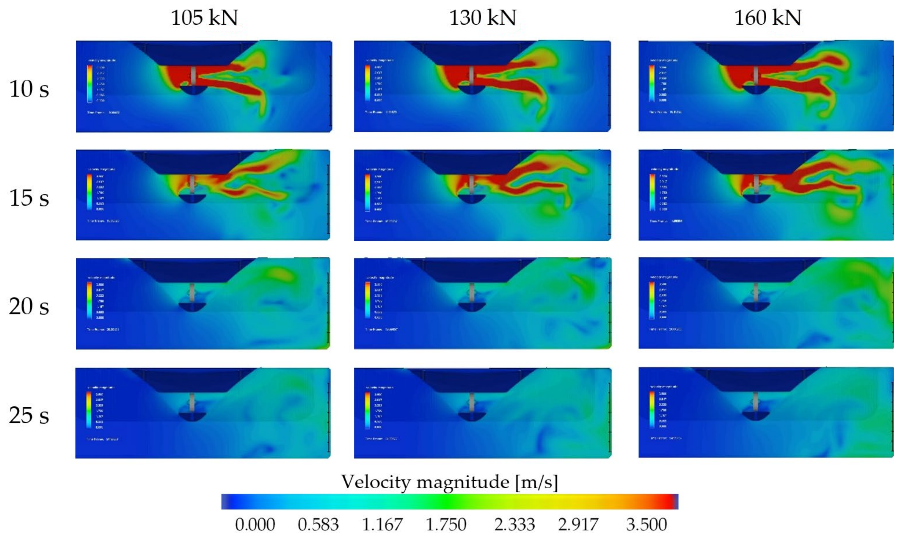
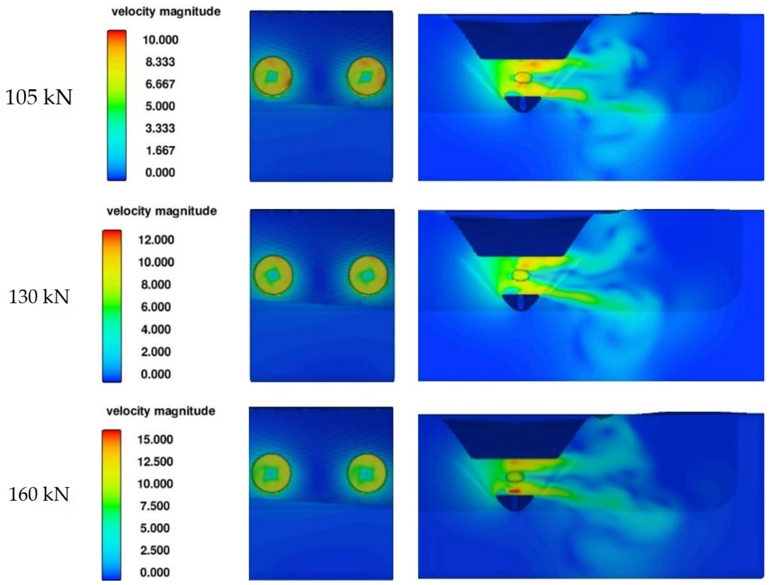
3.2. Velocity Field on the Quay Wall and Seabed
4. Conclusions
Author Contributions
Funding
Conflicts of Interest
References
- Van Blaaderen, E.A. Modelling Bowthruster Induced Flow near a Quay-Wall. TU Delft, Faculty of Civil Engineering and Geosciences, Hydraulic Engineering. 2006. Available online: https://repository.tudelft.nl/islandora/object/uuid:c5443985-9992-4de8-8505-f20456946799 (accessed on 27 October 2022).
- Van den Brink, A.J.W. Modelling of Scour Depth at Quay Walls due to Thrusters. Faculty of Civil Engineering and Geosciences. Hydraulik Engineering Dept. 2014. Available online: https://repository.tudelft.nl/islandora/object/uuid%3A57693312-4315-45ff-bf56-82551871dc52 (accessed on 27 October 2022).
- Abramowicz-Gerigk, T.; Burciu, Z.; Jachowski, J.; Kreft, O.; Majewski, D.; Stachurska, B.; Sulisz, W.; Szmytkiewicz, P. Experimental Method for the Measurements and Numerical Investigations of Force Generated on the Rotating Cylinder under Water Flow. Sensors 2021, 21, 2216. [Google Scholar] [CrossRef] [PubMed]
- PIANC. Guidelines for protecting berthing structures from scour caused by ships. The World Association for Waterborne Transport Infrastructure (PIANC), Maritime Navigation Commission Report No. 180. Marcom Rep. 2015, 180. Available online: https://www.pianc.org (accessed on 27 October 2022).
- Gucma, S.; Gucma, M. Optimization of LNG terminal parameters for a wide range of gas tanker sizes: The case of the port of Swinoujscie. Arch. Transp. 2019, 50, 91–100. [Google Scholar] [CrossRef]
- Hawkswood, M.G.; Lafeber, F.H.; Hawkswood, G.M. Berth Scour Protection for Modern Vessels by PIANC World Congress San Francisco USA. 2014. Available online: https://proserveltd.co.uk/wp-content/uploads/2020/08/2014-Paper-Berth-Scour-Protection-for-Modern-Vessels.pdf (accessed on 27 October 2022).
- Abramowicz-Gerigk, T.; Burciu, Z. Gdynia Maritime University. Measuring System of Pressure Distribution on the Surface of Hydrotechnical Constructions. Patent PL 235914, Patent Office of the Republic of Poland: Warsaw, Poland Patent Granted on 16 November 2020. Available online: https://api-ewyszukiwarka.pue.uprp.gov.pl/api/collection/fb6a3bce9cd3b66bb0d2e9b06d623399#search=%22P.409435%22 (accessed on 27 October 2022).
- Abramowicz-Gerigk, T.; Burciu, Z.; Gorski, W.; Reichel, M. Full scale measurements of pressure field induced on the quay wall by bow thrusters–indirect method for seabed velocities monitoring. Ocean Eng. 2018, 162, 150–160. [Google Scholar] [CrossRef]
- Schmidt, E. Belastungen durch Bugstrahlruder. In Belastung, Stabilisierung und Befestigung von Sohlen und Böschungen wasserbaulicher Anlagen Dresdner Wasserbauliche Mitteilungen 18; Technische Universität Dresden, Institut für Wasserbau und Technische Hydromechanik: Dresden, Germany, 2000; pp. 145–168. Available online: https://core.ac.uk/download/pdf/326238445.pdf (accessed on 27 October 2022).
- Römisch, K. Der Propellerstrahl als erodierendes Element bei An-und Ablegmanövern im Hafenbecken. Seewirtschaft 1975, 7, 431–434. [Google Scholar]
- Yoo, W.-J.; Yoo, B.Y.; Rhee, K.P. An experimental study on the manoeuvring characteristics of a twin propeller/twin rudder ship during berthing and unberthing. Ships Offshore Struct. 2006, 1, 191–198. Available online: https://proserveltd.co.uk/wp-content/uploads/2020/08/2016-Paper-Propeller-Action-and-Berth-Scour-Protection-Hawkswood-et-al-2016.pdf (accessed on 27 October 2022). [CrossRef]
- Hwang, T.; Yeom, G.-S.; Seo, M.; Lee, C.; Lee, W.-D. Impact of the Thruster Jet Flow of Ultra-large Container Ships on the Stability of Quay Walls. J. Ocean. Eng. Technol. 2021, 35, 403–413. [Google Scholar] [CrossRef]
- Cui, Y.; Lam, W.H.; Puay, H.T.; Ibrahim, M.S.; Robinson, D.; Hamill, G. Component Velocities and Turbulence Intensities within Ship Twin-Propeller Jet Using CFD and ADV. J. Mar. Sci. Eng. 2020, 8, 1025. [Google Scholar] [CrossRef]
- Hsu, W. Assessing the Safety Factors of Ship Berthing Operations. J. Navig. 2015, 68, 576–588. [Google Scholar] [CrossRef]


| Parameter | Description |
|---|---|
| B [m] | ship breadth |
| DBT [m] | diameter of bow thruster |
| h [m] | water depth |
| L [m] | distance between the quay wall and bow thruster opening |
| LoA [m] | ship length overall |
| N [kW] | main engines power |
| NBT1 [kW] | power of the first bow thruster from the bow |
| NBT2 [kW] | power of the second bow thruster from the bow |
| NST [kW] | power of stern thruster |
| n [rpm] | bow thruster propeller revolutions |
| p [kPa] | pressure |
| T [m] | ship draft |
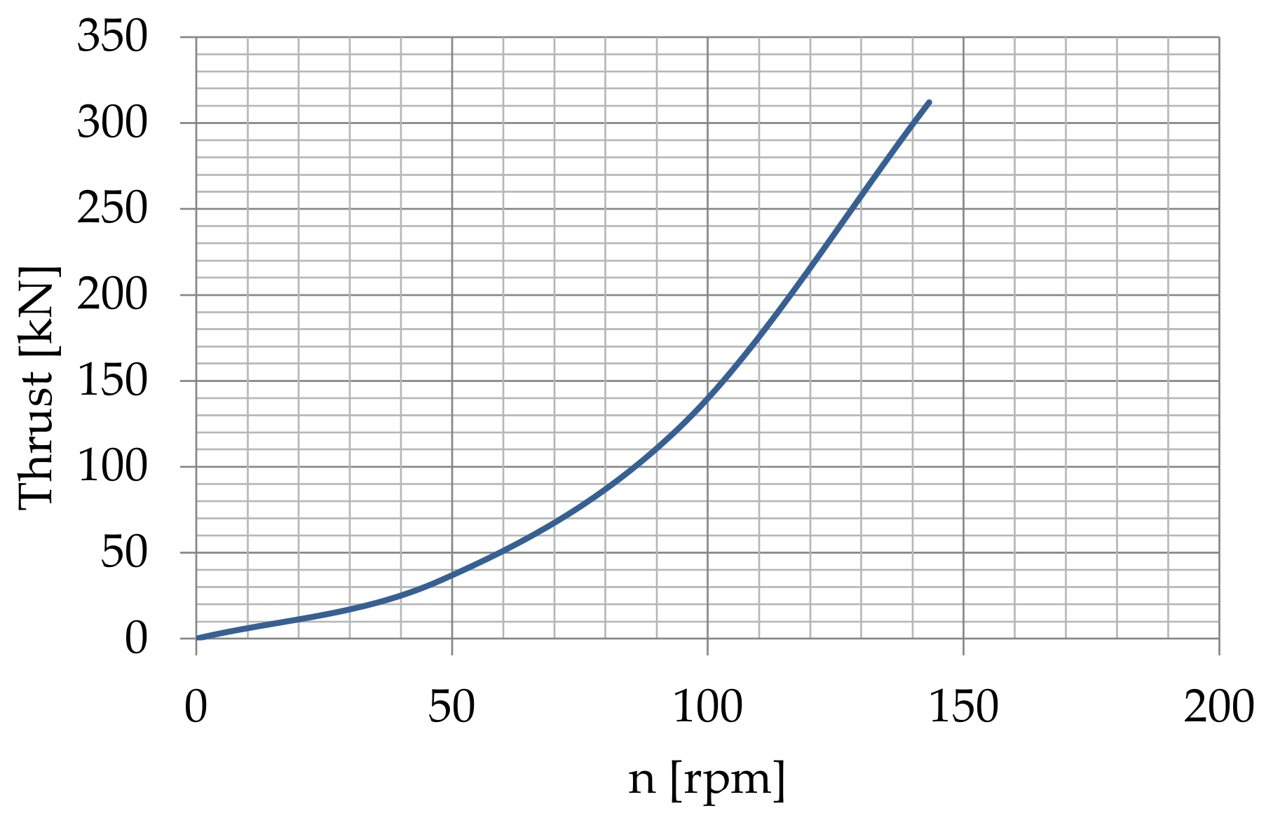
| Thrust [kN] | thrust of the bow thruster |
| t [s] | time of measurements |
| ts [s] | time of simulation |
| v [m/s] | flow velocity |
| v0 [m/s] | axial velocity of the bow thruster jet |
| z [m] | height of the bow thruster axis above the seabed |
| P [kg/m3] | water density |
| Parameter | Ferry 1 | Ferry 2 |
|---|---|---|
| LOA [m] | 164.41 | 175.48 |
| B [m] | 27.69 | 30.3 |
| T [m] | 6.313 | 6.8 |
| N [kW] | 4 × 4840 | 4 × 7454 |
| NBT1 [kW] | 1275 | 1119 |
| NBT2 [kW] | 735 | 1119 |
| NST [kW] | 735 | - |
| Impeller Properities | |
|---|---|
| Accomodation coefficient for rotational velocity | 14 |
| Axial velocity coefficient | −1.5 |
| Number of blades | 4 |
| Blade tip thickness in azimuthal direction [m] | 0.05 |
| Propeller revolution [rpm]/thrust [kN] | 86/105; 94/130; 104/160 |
| Bow thruster diameter [m] | 2.37 |
| Hub diameter [m] | 0.68 |
| Ferry | v0 | vmax | |||
|---|---|---|---|---|---|
| m/s | m/s | ||||
| Equation (3) | German Method | Dutch Method | CFD Simulation | Measurement | |
| Ferry 1 | 7.1 | 2.9 | 2.7 | 2.8 | 2.8 |
| Ferry 2 | 6.7 | 2.5 | 2.6 | 2.4 | 2.4 |
| Thrust | v0 | vmax | ||
|---|---|---|---|---|
| m/s | m/s | |||
| kN | CFD | CFD | German Method | Dutch Method |
| 105 | 5.3 | 2.1 | 2.0 | 2.0 |
| 130 | 5.7 | 2.2 | 2.1 | 2.2 |
| 160 | 6.7 | 2.6 | 2.5 | 2.6 |
Publisher’s Note: MDPI stays neutral with regard to jurisdictional claims in published maps and institutional affiliations. |
© 2022 by the authors. Licensee MDPI, Basel, Switzerland. This article is an open access article distributed under the terms and conditions of the Creative Commons Attribution (CC BY) license (https://creativecommons.org/licenses/by/4.0/).
Share and Cite
Abramowicz-Gerigk, T.; Jachowski, J. Ship Berthing and Unberthing Monitoring System in the Ferry Terminal. Sensors 2022, 22, 9133. https://doi.org/10.3390/s22239133
Abramowicz-Gerigk T, Jachowski J. Ship Berthing and Unberthing Monitoring System in the Ferry Terminal. Sensors. 2022; 22(23):9133. https://doi.org/10.3390/s22239133
Chicago/Turabian StyleAbramowicz-Gerigk, Teresa, and Jacek Jachowski. 2022. "Ship Berthing and Unberthing Monitoring System in the Ferry Terminal" Sensors 22, no. 23: 9133. https://doi.org/10.3390/s22239133
APA StyleAbramowicz-Gerigk, T., & Jachowski, J. (2022). Ship Berthing and Unberthing Monitoring System in the Ferry Terminal. Sensors, 22(23), 9133. https://doi.org/10.3390/s22239133