
Development and Calibration of a Low-Cost, Piezoelectric Rainfall Sensor through Machine Learning

 ,
,  ,
,  , ,
, ,  and
and
Abstract
:1. Introduction
2. Materials and Methods
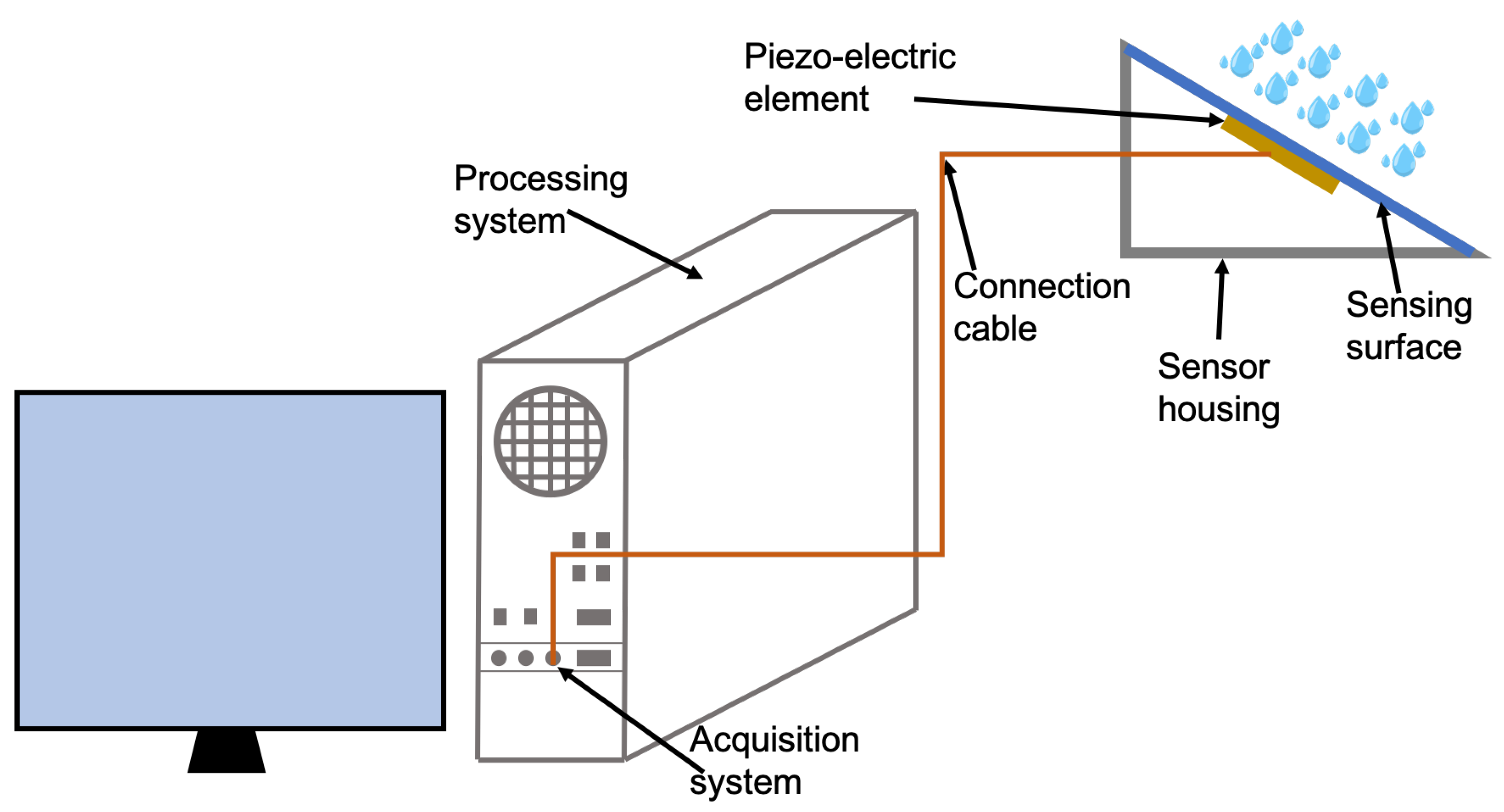
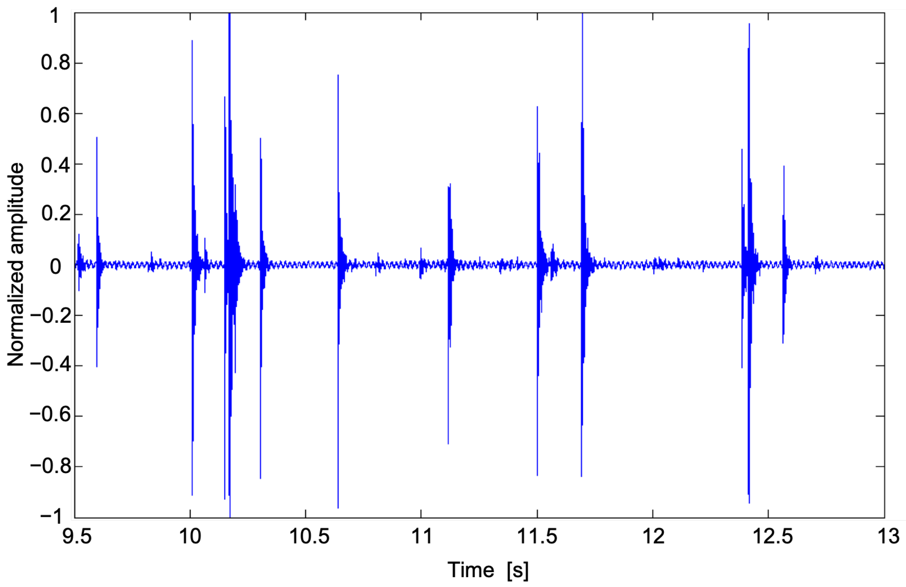
2.1. Instrument Prototype Setup and Signal Processing
2.2. Calibration with Machine-Learning Methods
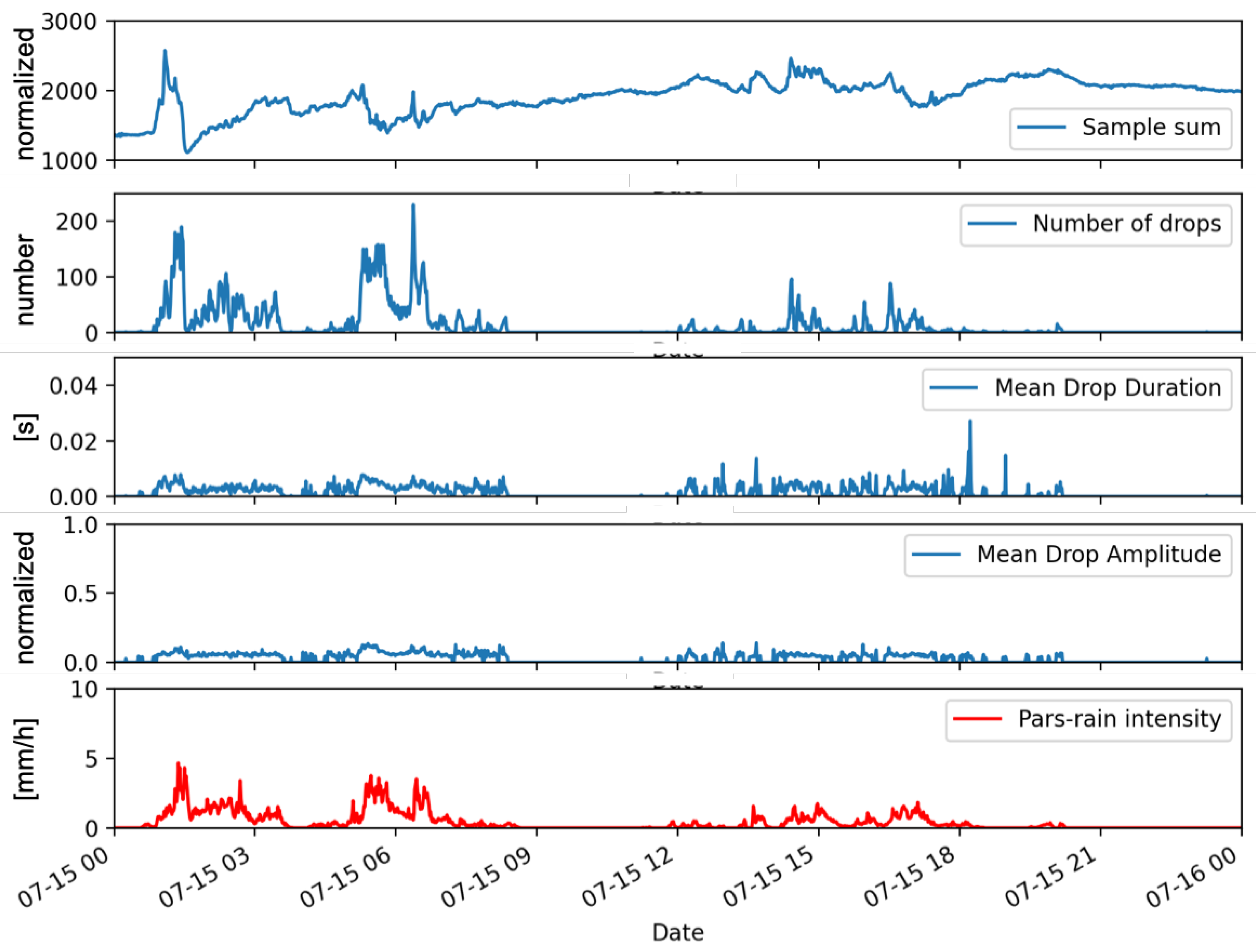
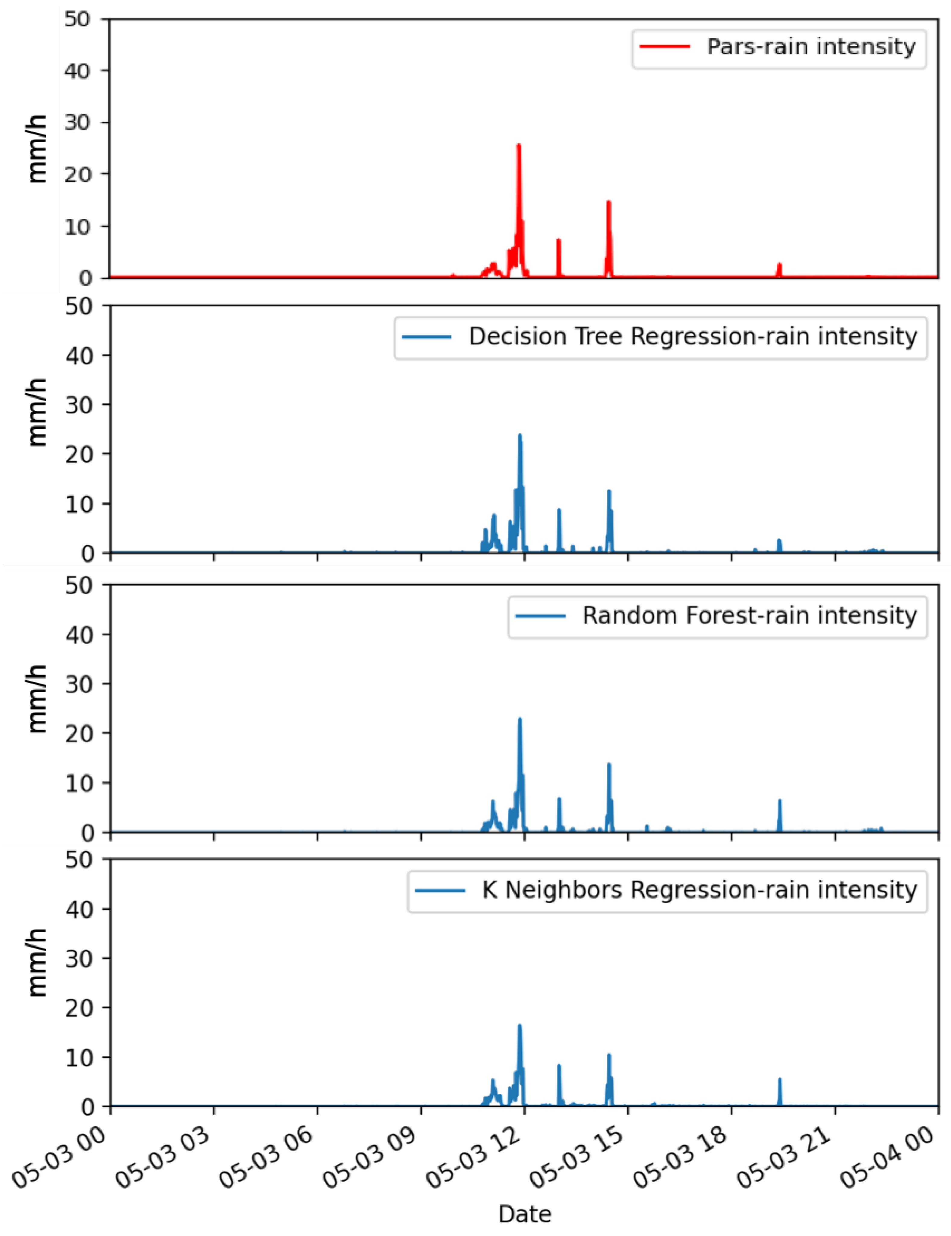
3. Results
4. Conclusions and Future Works
Author Contributions
Funding
Institutional Review Board Statement
Informed Consent Statement
Data Availability Statement
Conflicts of Interest
References
- Lanza, L.G.; Cauteruccio, A.; Stagnaro, M. Chapter 4—Rain gauge measurements. In Rainfall; Morbidelli, E., Ed.; Elsevier: Amsterdam, The Netherlands, 2022; pp. 77–108. [Google Scholar] [CrossRef]
- Kathiravelu, G.; Lucke, T.; Nichols, P. Rain Drop Measurement Techniques: A Review. Water 2016, 1, 29. [Google Scholar] [CrossRef]
- Jameson, A.R.; Larsen, M.L.; Kostinski, A.B. An example of persistent microstructure in a long rain event. J. Hydrometeorol. 2016, 17, 1661–1673. [Google Scholar] [CrossRef]
- Friedrich, K.; Kalina, E.A.; Aikins, J.; Steiner, M.; Gochis, D.; Kucera, P.A.; Ikeda, K.; Sun, J. Raindrop size distribution and rain characteristics during the 2013 Great Colorado Flood. J. Hydrometeorol. 2013, 17, 53–72. [Google Scholar] [CrossRef]
- Bringi, V.N.; Tolstoy, L.; Thurai, M.; Petersen, W.A. Estimation of spatial correlation of drop size distribution parameters and rain rate using NASA’s S-band polarimetric radar and 2D video disdrometer network: Two case studies from MC3E. J. Hydrometeorol. 2015, 16, 1207–1221. [Google Scholar] [CrossRef]
- Anagnostou, M.N.; Kalogiros, J.; Marzano, F.S.; Anagnostou, E.N.; Montopoli, M.; Picciotti, E. Performance evaluation of a new dual-polarization microphysical algorithm based on long-term X-band radar and disdrometer observations. J. Hydrometeorol. 2013, 14, 560–576. [Google Scholar] [CrossRef]
- Adirosi, E.; Roberto, N.; Montopoli, M.; Gorgucci, E.; Baldini, L. Influence of disdrometer type on weather radar algorithms from measured DSD: Application to Italian climatology. Atmosphere 2018, 9, 360. [Google Scholar] [CrossRef]
- Adirosi, E.; Montopoli, M.; Bracci, A.; Porcù, F.; Capozzi, V.; Annella, C.; Budillon, G.; Bucchignani, E.; Zollo, A.L.; Cazzuli, O.; et al. Validation of GPM Rainfall and Drop Size Distribution Products through Disdrometers in Italy. Remote Sens. 2021, 13, 2081. [Google Scholar] [CrossRef]
- Joss, J.; Waldvogel, A. Ein spektrograph für niederschlagstropfen mit automatischer auswertung. Pure Appl. Geophys. 1967, 68, 240–246. [Google Scholar] [CrossRef]
- Salmi, A.; Ikonen, J. Piezoelectric precipitation sensor from Vaisala. In Proceedings of the World Meteorology Organization Technical Conference on Meteorological and Environmental Instruments and Methods of Observation (TECO 2005), Bucharest, Romania, 4–7 May 2005; World Meteorological Organization: Geneva, Switzerland, 2005. [Google Scholar]
- Abd Elbasit, M.A.M.; Yasuda, H.; Salmi, A. Application of piezoelectric transducers in simulated rainfall erosivity assessment. Hydrol. Sci. J. 2011, 56, 187–194. [Google Scholar] [CrossRef]
- Kundgol, A. A Novel Technique for Measuring and Sensing Rain. Ph.D. Thesis, School of Computing, Science and Engineering, University of Salford, Salford, UK, 2015. [Google Scholar]
- Cuccoli, F.; Facheris, L.; Antonini, A.; Melani, S.; Baldini, L. Weather Radar and Rain-Gauge Data Fusion for Quantitative Precipitation Estimation: Two Case Studies. IEEE Trans. Geosci. Remote Sens. 2020, 58, 6639–6649. [Google Scholar] [CrossRef]
- Vas, A.; Fazekas, A.; Nagy, I.; Tóth, L. Distributed Sensor Network for meteorological observations and numerical weather Prediction Calculations. Carpathian J. Electron. Comput. Eng. 2013, 6, 56–63. [Google Scholar]
- Croci, A. A Novel Approach to Rainfall Measuring: Methodology, Field Test Andbusiness Opportunity; Doctoral Program in Environmental Engineering (29th Cycle); Politecnico di Torino: Torino, Italy, 2017. [Google Scholar]
- Bernardes, G.F.L.R.; Ishibashi, R.; de Souza Ivo, A.A.; Rosset, V.; Kimura, B.Y.L. Prototyping Low-Cost automatic weather stations for natural disaster monitoring. Digit. Commun. Netw. 2022. [Google Scholar] [CrossRef]
- Fang, X. Improving Data Quality for Low-Cost Environmental Sensors. Ph.D. Thesis, University of York Computer Science, York, UK, April 2018. [Google Scholar]
- Okafor, N.U.; Alghorani, Y.; Delaney, D.T. Improving data quality of low-cost IoT sensors in environmental monitoring networks using data fusion and machine learning approach. ICT Express 2020, 6, 220–228. [Google Scholar] [CrossRef]
- Yamamoto, K.; Togami, T.; Yamaguchi, N.; Ninomiya, S. Machine Learning-based calibration of low-cost air temperature sensors using environmental data. Sensors 2017, 17, 1290. [Google Scholar] [CrossRef] [PubMed]
- Killingsworth, J.A. The PC Sound Card as a Voltage Measurement Platform in Power System Applications. Ph.D. Thesis, Auburn University, Auburn, AL, USA, 13 December 2014. [Google Scholar]
- De Jong, S. Low Cost Disdrometer Improved Design and Testing in an Urban Environment. Master’s Thesis, Delft University of Technology, Delft, The Netherlands, December 2010. [Google Scholar]
- Binotto, A.; Albuquerque de Castro, B.; Vecina dos Santos, V.; Alfredo Ardila Rey, J.; Luiz Andreoli, A. A Comparison between Piezoelectric Sensors Applied to Multiple Partial Discharge Detection by Advanced Signal Processing Analysis. In Proceedings of the 7th International Electronic Conference on Sensors and Applications, Online, 15–30 November 2020. [Google Scholar]
- Zimmerman, N.; Presto, A.A.; Kumar, S.P.; Gu, J.; Hauryliuk, A.; Robinson, E.S.; Robinson, A.L.; Subramanian, R. A machine learning calibration model using Random Forests to improve sensor performance for lower-cost air quality monitoring. Atmos. Meas. Tech. 2018, 11, 291–313. [Google Scholar] [CrossRef]
- Pedregosa, F.; Varoquaux, G.; Gramfort, A.; Michel, V.; Thirion, B.; Grisel, O.; Blondel, M.; Prettenhofer, P.; Weiss, R.; Dubourg, V.; et al. Scikit-learn: Machine Learning in Python. J. Mach. Learn. Res. 2011, 12, 2825–2830. [Google Scholar]
- Johannsen, L.L.; Zambon, N.; Strauss, P.; Dostal, T.; Neumann, M.; Zumr, D.; Cochrane, T.A.; Blöschl, G.; Klik, A. Comparison of three types of laser optical disdrometers under natural rainfall conditions. Hydrol. Sci. J. 2020, 65, 524–535. [Google Scholar] [CrossRef] [PubMed]


| Method | MAE Train (mm/h) | MAE Test (mm/h) |
|---|---|---|
| Linear Regression | 0.15 | 0.13 |
| Partial Least Squares Regression | 0.17 | 0.15 |
| Support Vector Regression | 0.14 | 0.13 |
| Decision Tree Regression | <0.01 | 0.06 |
| Random Forest | 0.02 | 0.05 |
| K Neighbors Regression | 0.05 | 0.04 |
| Neural Network MLPR | 0.17 | 0.15 |
| Method | MAE in May and July |
|---|---|
| Decision Tree Regression | 0.11 |
| Random Forest | 0.08 |
| K Neighbors Regression | 0.08 |
Publisher’s Note: MDPI stays neutral with regard to jurisdictional claims in published maps and institutional affiliations. |
© 2022 by the authors. Licensee MDPI, Basel, Switzerland. This article is an open access article distributed under the terms and conditions of the Creative Commons Attribution (CC BY) license (https://creativecommons.org/licenses/by/4.0/).
Share and Cite
Antonini, A.; Melani, S.; Mazza, A.; Baldini, L.; Adirosi, E.; Ortolani, A. Development and Calibration of a Low-Cost, Piezoelectric Rainfall Sensor through Machine Learning. Sensors 2022, 22, 6638. https://doi.org/10.3390/s22176638
Antonini A, Melani S, Mazza A, Baldini L, Adirosi E, Ortolani A. Development and Calibration of a Low-Cost, Piezoelectric Rainfall Sensor through Machine Learning. Sensors. 2022; 22(17):6638. https://doi.org/10.3390/s22176638
Chicago/Turabian StyleAntonini, Andrea, Samantha Melani, Alessandro Mazza, Luca Baldini, Elisa Adirosi, and Alberto Ortolani. 2022. "Development and Calibration of a Low-Cost, Piezoelectric Rainfall Sensor through Machine Learning" Sensors 22, no. 17: 6638. https://doi.org/10.3390/s22176638
APA StyleAntonini, A., Melani, S., Mazza, A., Baldini, L., Adirosi, E., & Ortolani, A. (2022). Development and Calibration of a Low-Cost, Piezoelectric Rainfall Sensor through Machine Learning. Sensors, 22(17), 6638. https://doi.org/10.3390/s22176638