
Efficient Obstacle Detection and Tracking Using RGB-D Sensor Data in Dynamic Environments for Robotic Applications

 , , ,
, , ,
Abstract
:1. Introduction
2. Literature Survey and Motivation of the Work
- We use dynamic binary thresholding on u-depth maps to improve obstacle detection and their accurate dimension estimation;
- We use restricted v-depth map representation for accurate estimation of obstacle dimensions;
- We present an algorithm for obstacle tracking using efficient processing of u-depth maps;
- The performance of the proposed system on different data sets establishes that the proposed system can detect and estimate the states of multiple static and dynamic obstacles more accurately and faster than SoA algorithms.
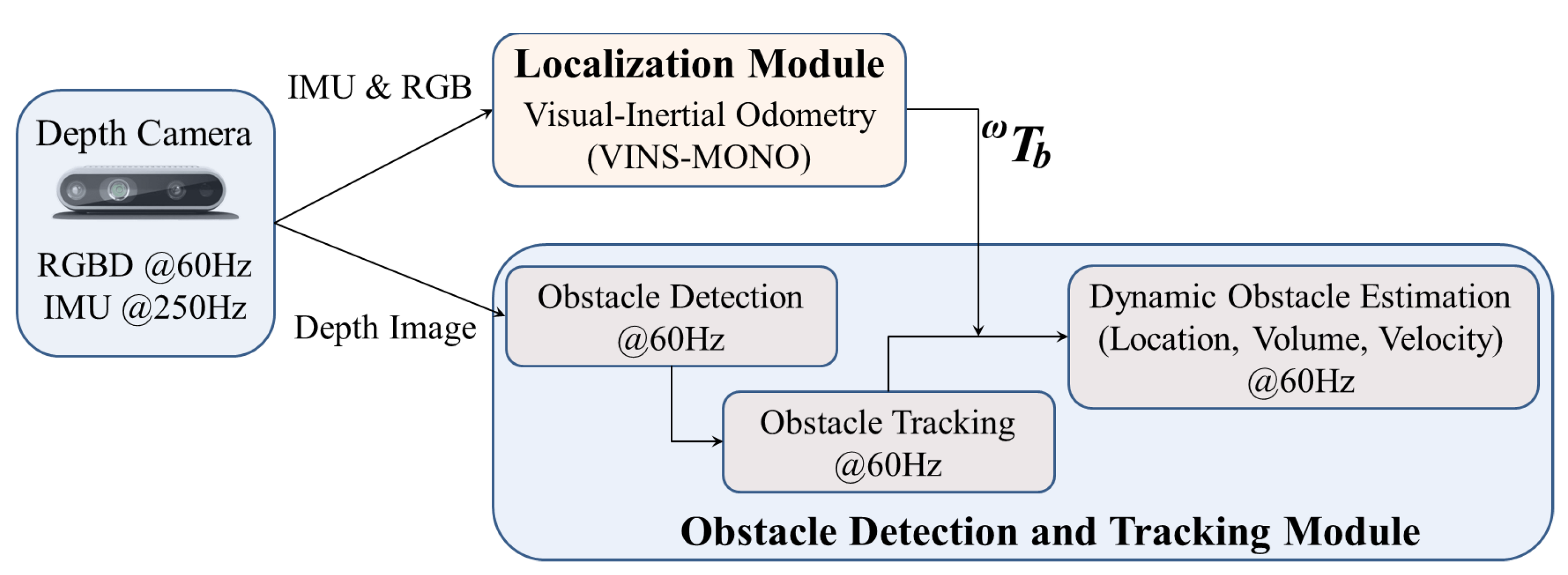
3. System Architecture
3.1. Self Localization
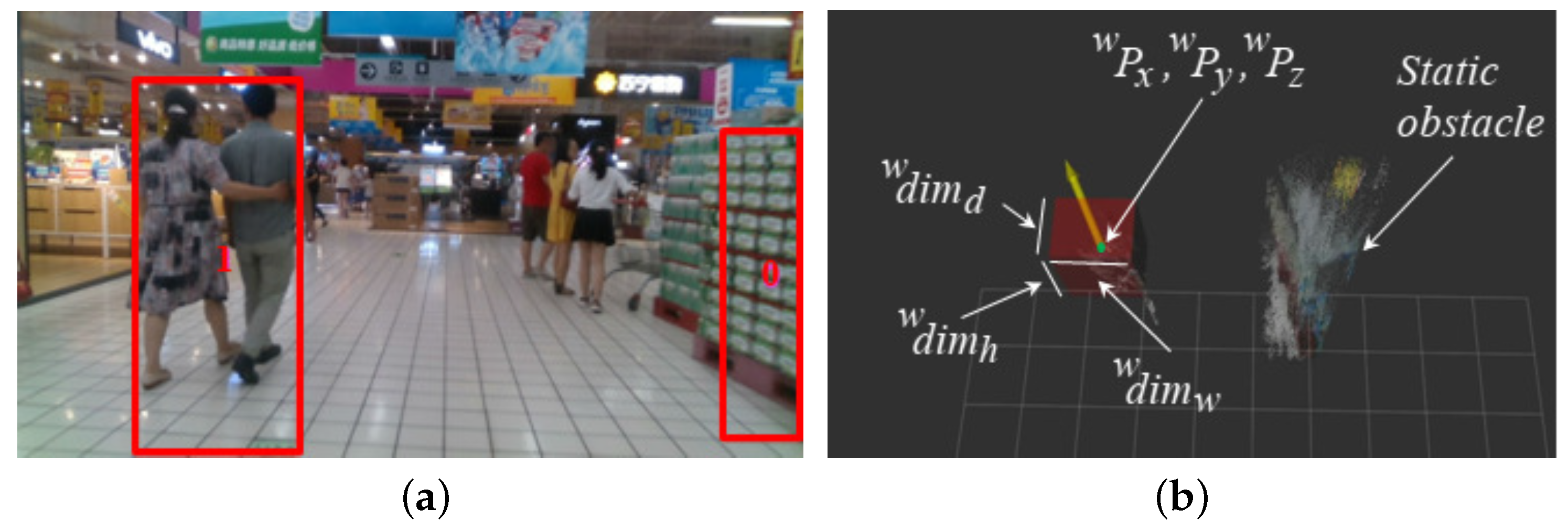
3.2. Obstacle Detection
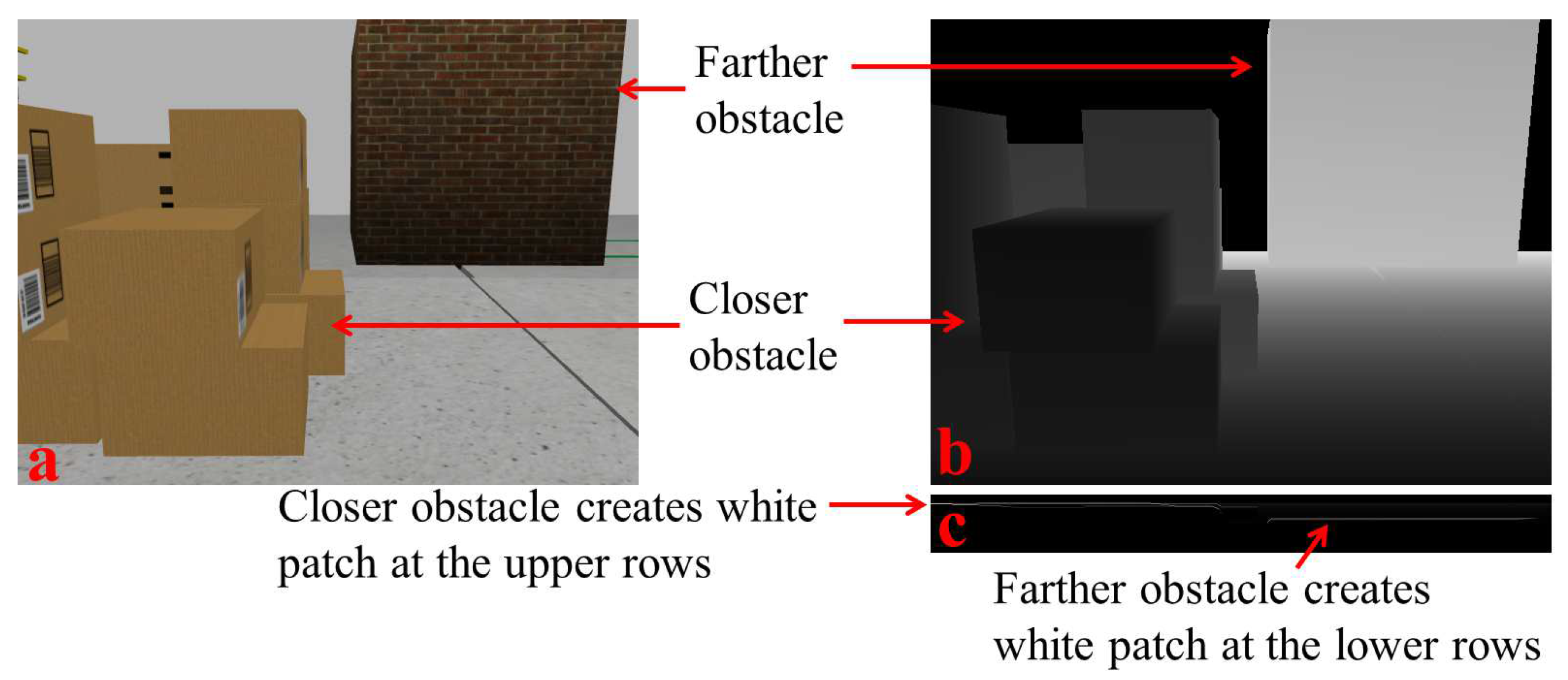
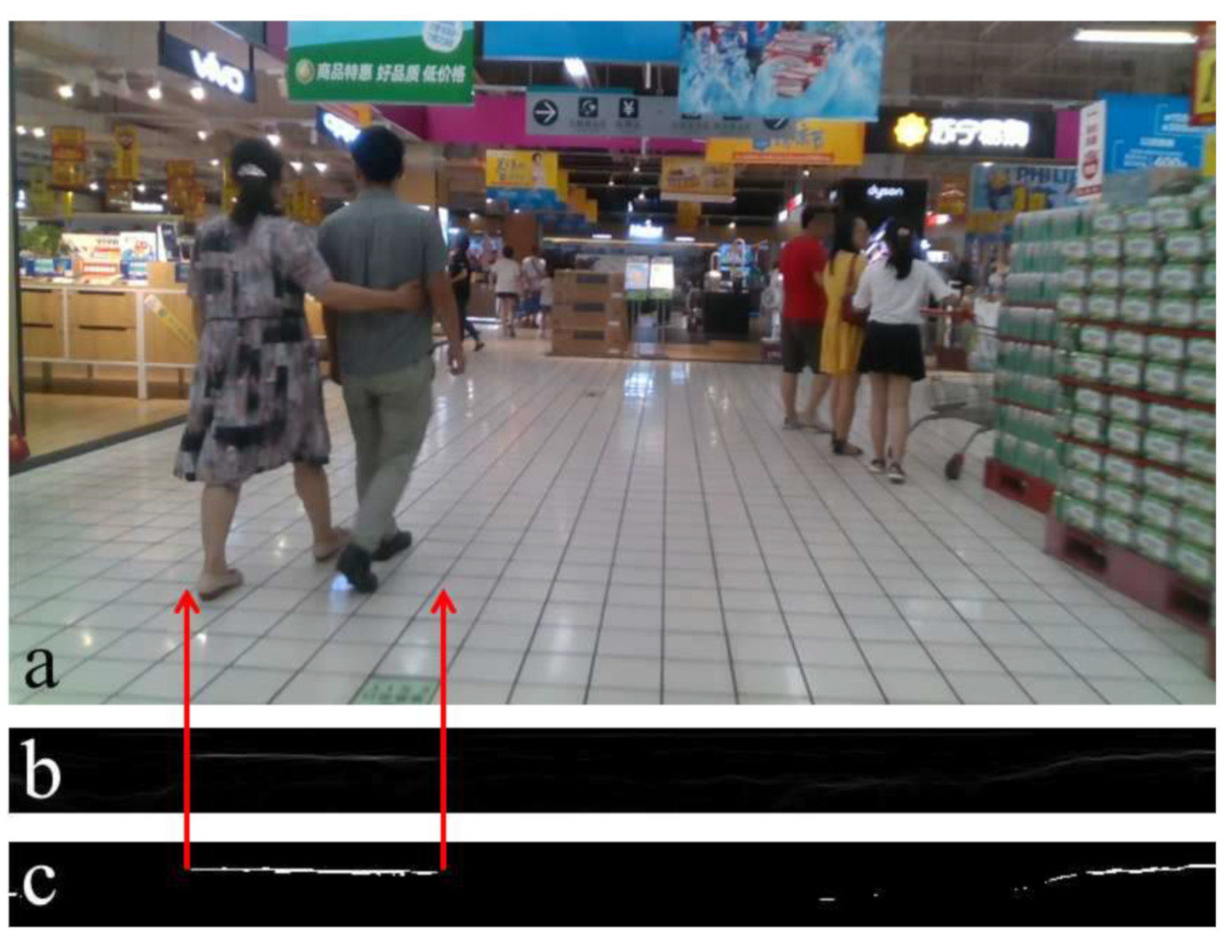
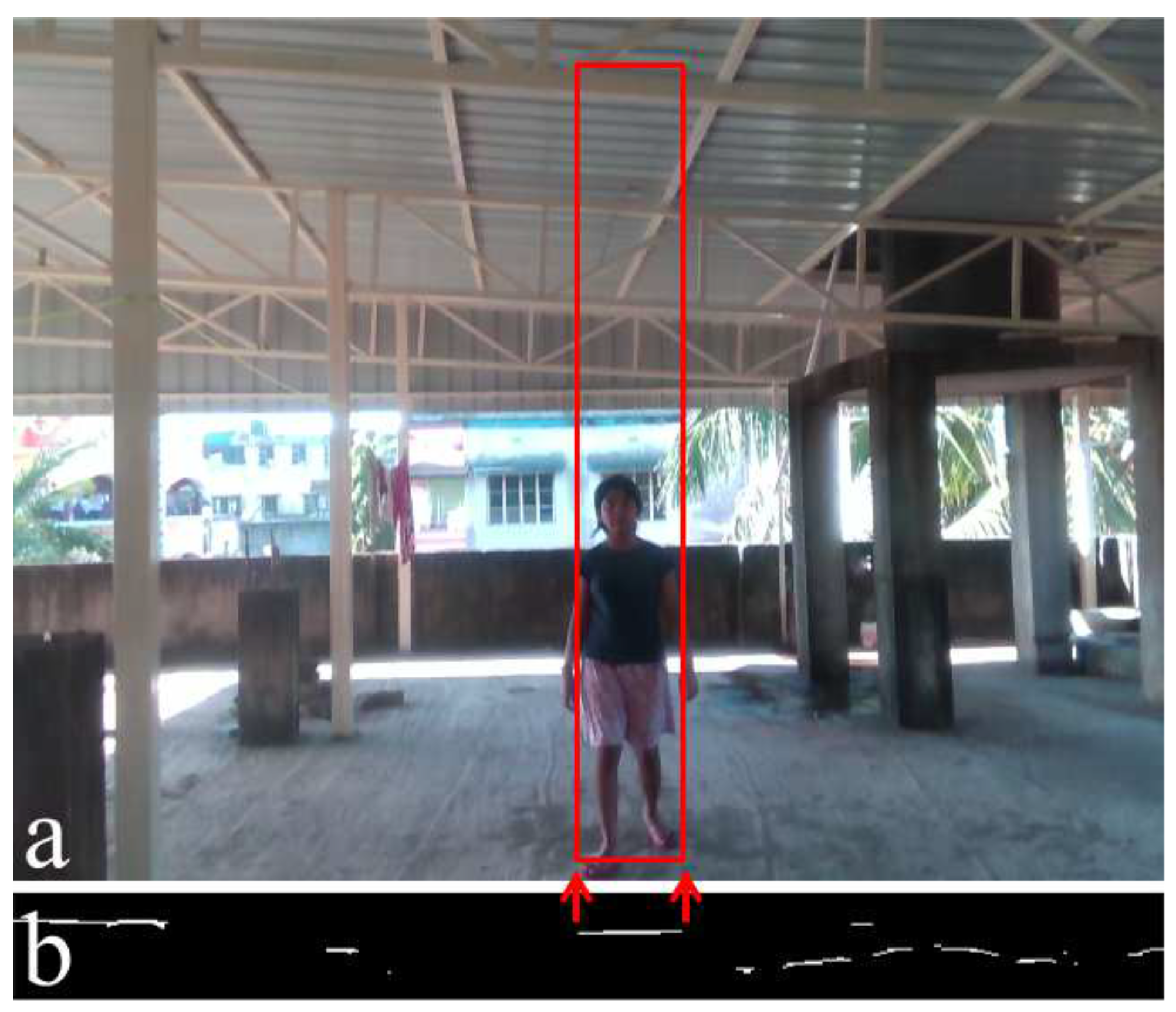
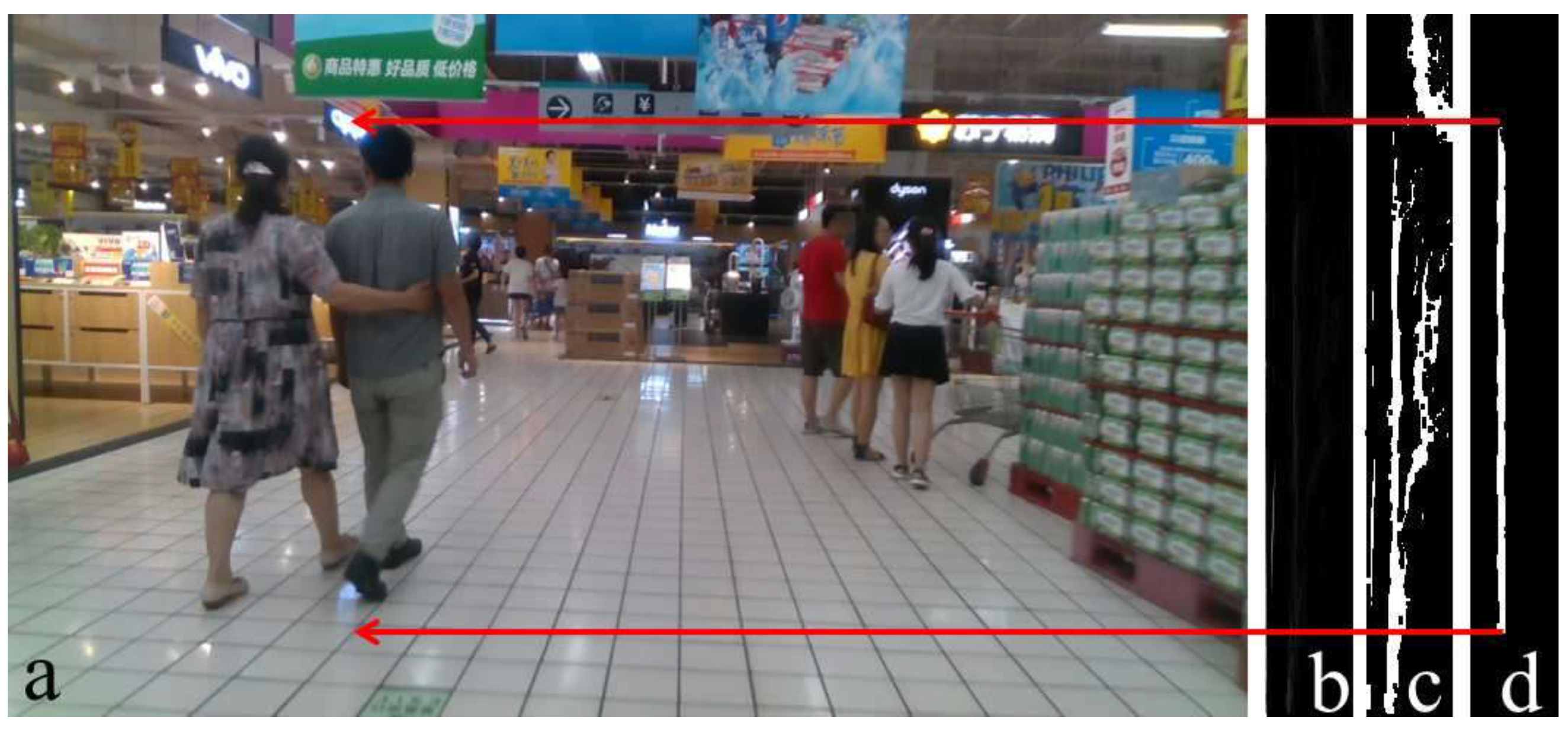
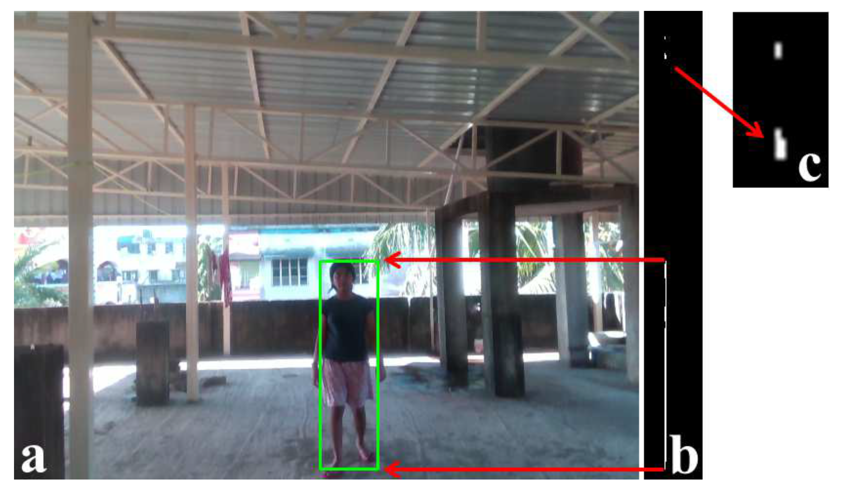
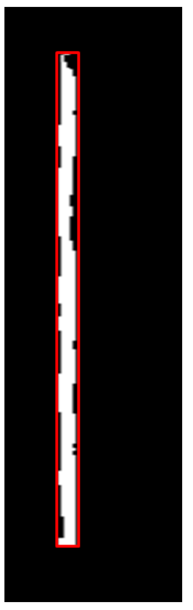
3.2.1. Depth Map Processing
| Algorithm 1: U-Depth Map (IMGd, N, Mind, Maxd, uScale) |
| Input: depth image , number of bins N, sensor depth range [], scaling factor Output: u-depth map Step 1. Step 2. for i = 1 to W for j = 1 to H If Step 3. Step 4. Return |
3.2.2. Dimension Calculation
| Algorithm 2: Restricted V-Depth Map () |
| Input: depth image , number of bins N, column range [], sensor depth range [], obstacle’s depth range [] Output: Thresholded v-depth map Step 1. Step 2. for i = 1 to H for j = to () If Step 3. Step 4. Return |
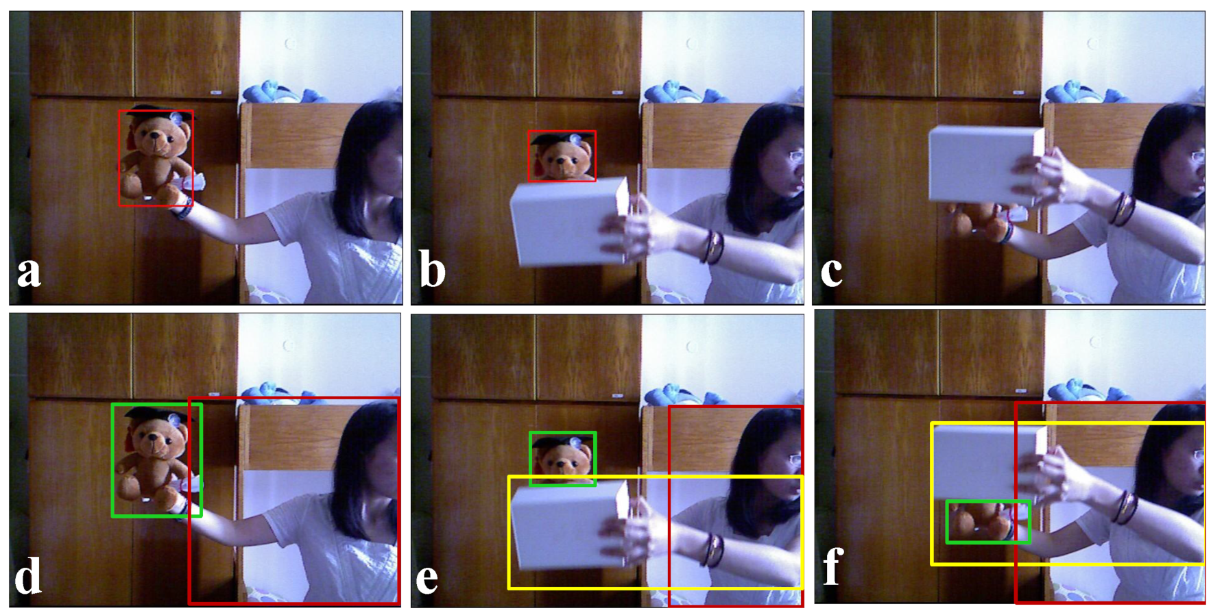
3.3. Obstacle Tracking
- If at least one of the matching obstacle from obstacles A and B is fully visible, is below a threshold , and the horizontal component of is also below a very small threshold , then we consider , , and to be zero because this is the case where the obstacle A almost stays at its previous position, and the width of the obstacle closely matches even after full visibility in one frame.
- If at least one of the matching obstacle from obstacles A and B is fully visible, and only is below the threshold , then we consider and to be zero because this is the case where obstacle A moves from its previous position, but the width of the obstacle matches closely even after complete visibility in one frame.
- If at least one of the matching obstacle from obstacles A and B is fully visible, and only the horizontal component of is below the threshold , then we consider to be zero because this is the case where the obstacle A does not move much, but there is a width change due to partial visibility in one frame.
- If both obstacles A and B are partially visible, is below a threshold . and the horizontal component of is also below a very small threshold , then we consider and to be zero because this is the case where obstacle A almost stays at its previous position, and the widths of the obstacles closely match in partial visibilities.
4. Experimental Results
4.1. Parameter Tuning
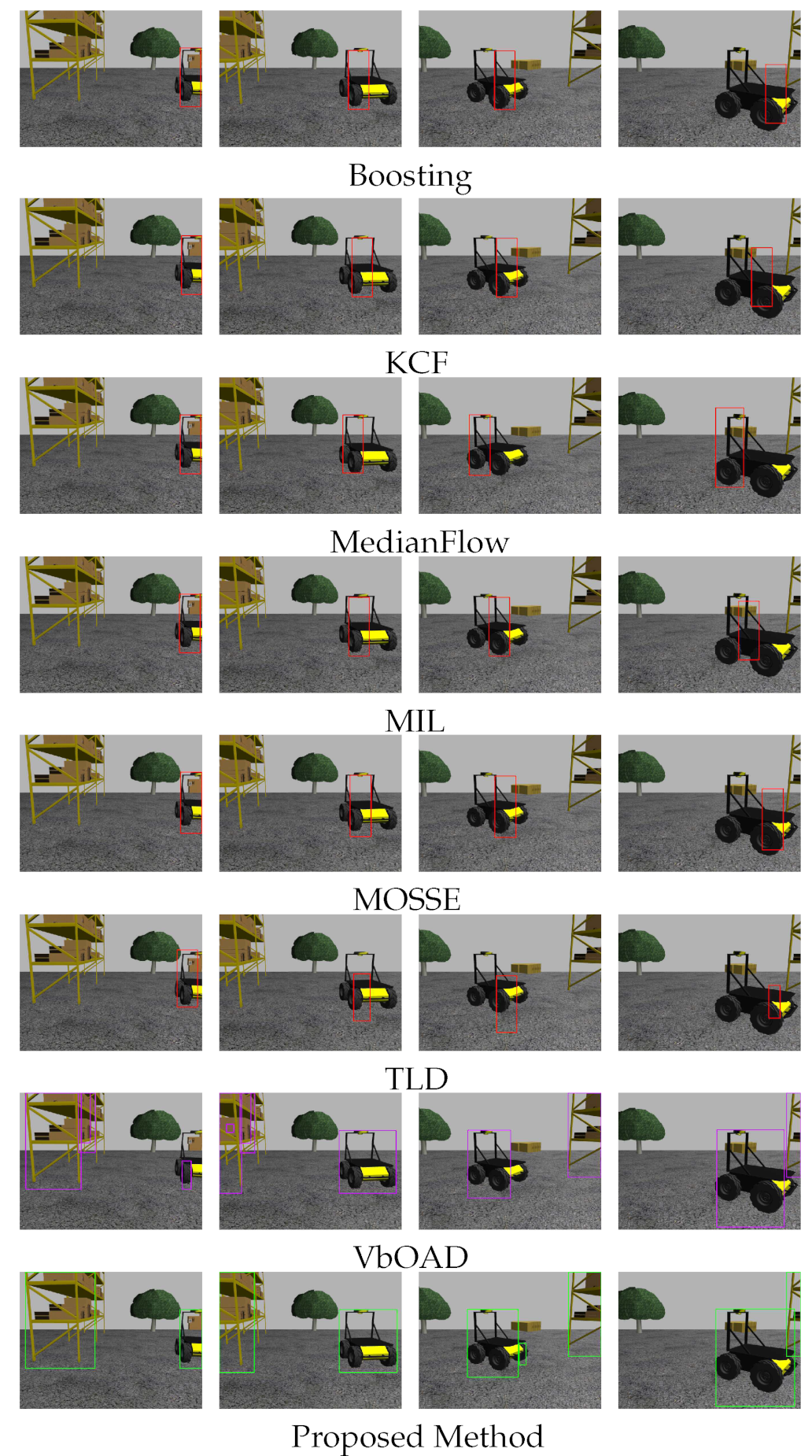
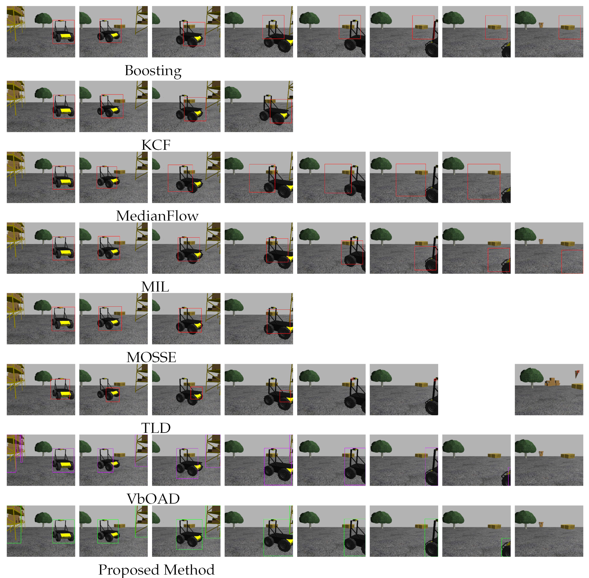
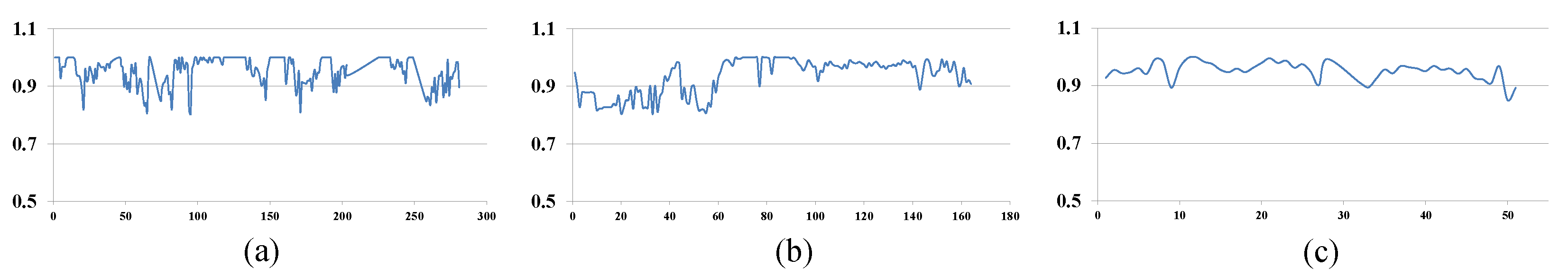
4.2. Obstacle Tracking Accuracy
4.2.1. Gazebo Environment and Experimental Set-Up
4.2.2. Initialization at Partial Visibility of Husky2
4.2.3. Initialization at Full Visibility of Husky2
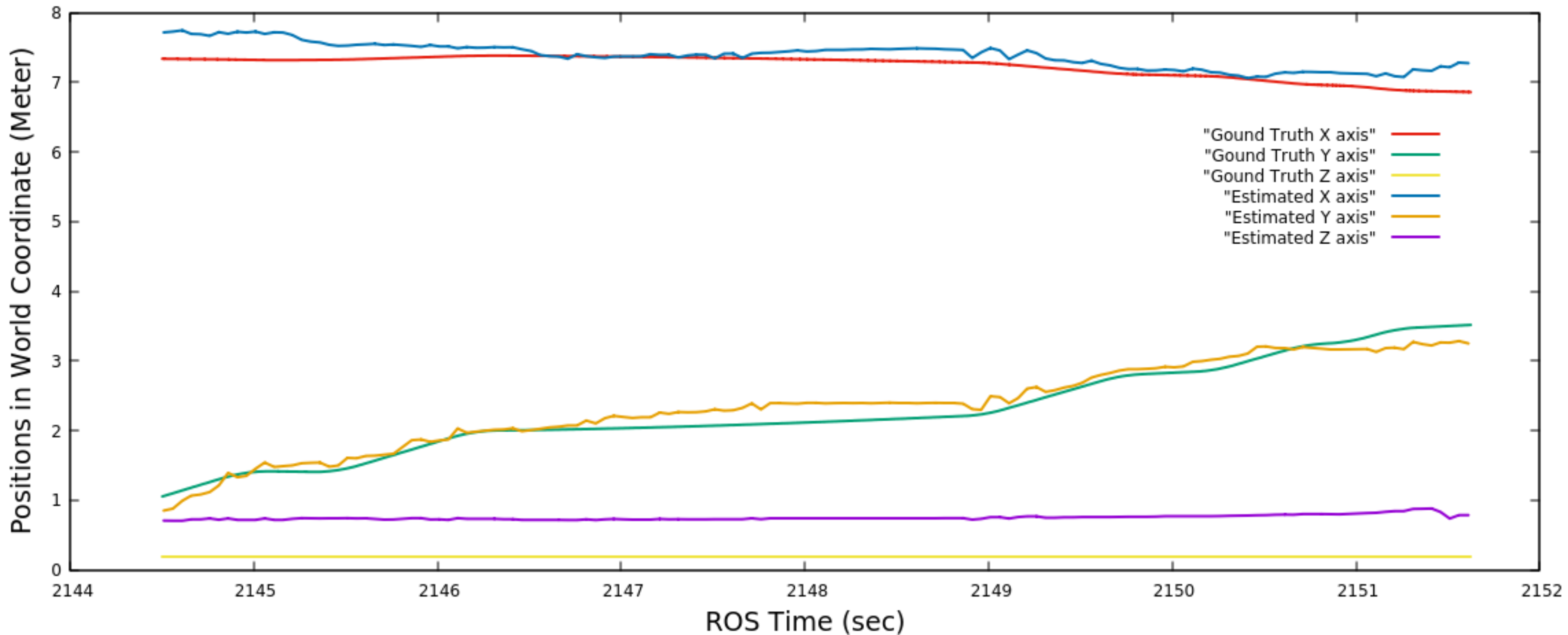
4.2.4. Accuracy Comparison on
4.2.5. Accuracy of the Proposed Method for and
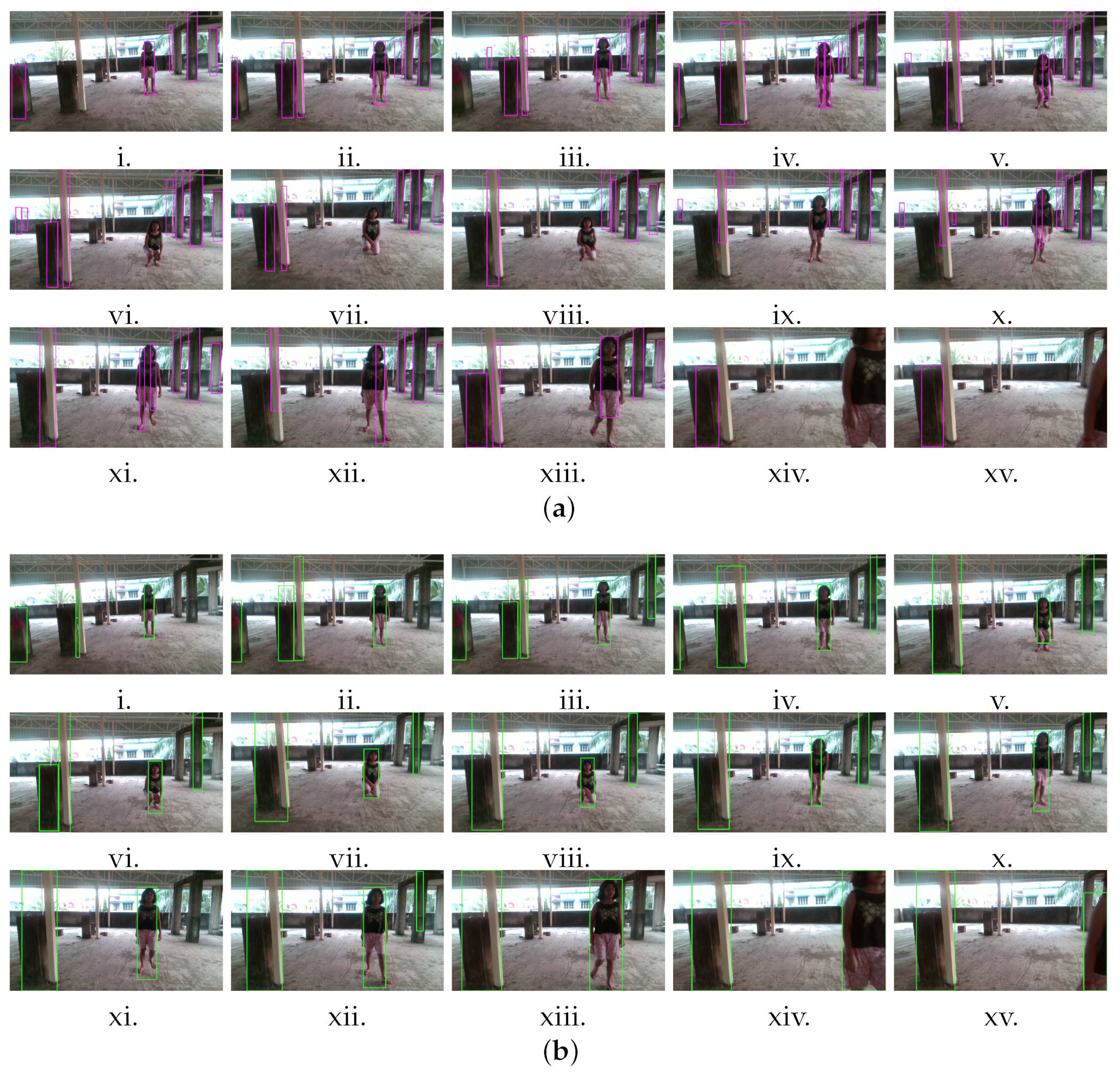
4.3. Dynamic Obstacles and Dynamic Size
4.3.1. Single Dynamic Obstacle with Varying Height ()
4.3.2. Multiple Obstacles with Different Heights ()
4.4. Accuracy Improvement with Dynamic U-Depth Thresholding on
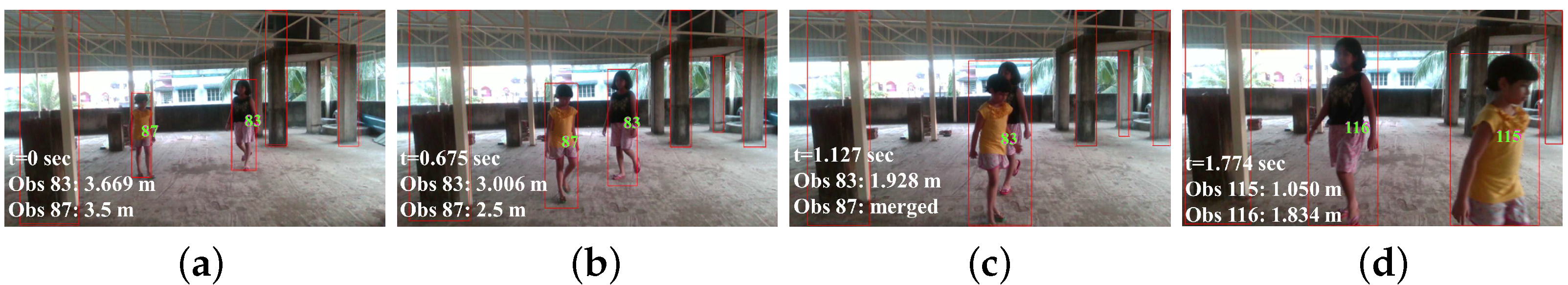
4.5. Experiments with Multiple Dynamic Obstacles ()
4.6. Indoor Open Sequence ()
4.7. Experiments with a Fast-Moving Obstacle ()
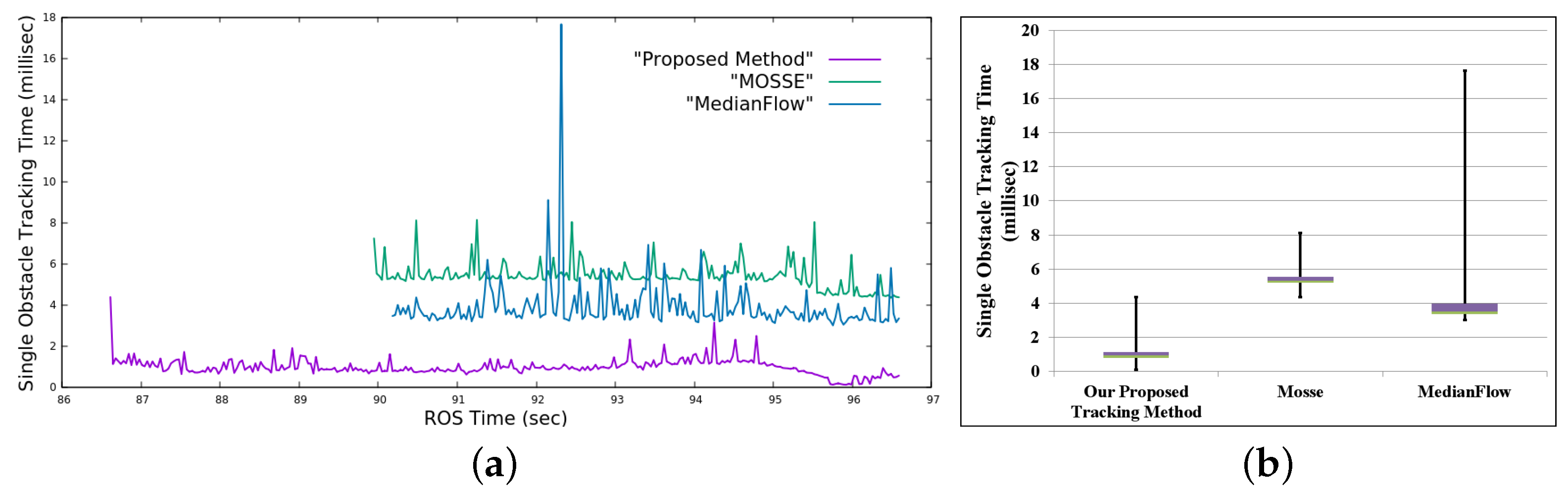
4.8. Execution Time
5. Conclusions
Author Contributions
Funding
Institutional Review Board Statement
Informed Consent Statement
Data Availability Statement
Conflicts of Interest
References
- Song, S.; Xiao, J. Tracking Revisited Using RGBD Camera: Unified Benchmark and Baselines. In Proceedings of the IEEE International Conference on Computer Vision, Sydney, Australia, 1–8 December 2013; pp. 233–240. [Google Scholar] [CrossRef]
- Gibbs, G.; Jia, H.; Madani, I. Obstacle Detection with Ultrasonic Sensors and Signal Analysis Metrics. Transp. Res. Procedia 2017, 28, 173–182. [Google Scholar] [CrossRef]
- Beltran, D.; Basañez, L. A Comparison between Active and Passive 3D Vision Sensors: BumblebeeXB3 and Microsoft Kinect. Adv. Intell. Syst. Comput. 2013, 252, 725–734. [Google Scholar]
- Labayrade, R.; Aubert, D.; Tarel, J. Real time obstacle detection on non flat road geometry through v-disparity representation. In Proceedings of the IEEE Intelligent Vehicles Symposium, Versailles, France, 17–21 June 2002. [Google Scholar]
- Labayrade, R.; Aubert, D. In-vehicle obstacles detection and characterization by stereovision. In Proceedings of the 1st International Workshop on In-Vehicle Cognitive Computer Vision Systems, Graz, Austria, 3rd April 2003; pp. 13–19. [Google Scholar]
- Oleynikova, H.; Honegger, D.; Pollefeys, M. Reactive avoidance using embedded stereo vision for MAV flight. In Proceedings of the IEEE International Conference on Robotics and Automation, Seattle, WA, USA, 26–30 May 2015; Volume 2015, pp. 50–56. [Google Scholar]
- Bertozzi, M.; Broggi, A.; Fascioli, A.; Nichele, S. Stereo vision-based vehicle detection. In Proceedings of the IEEE Intelligent Vehicles Symposium 2000 (Cat. No.00TH8511), Dearborn, MI, USA, 5 October 2000; pp. 39–44. [Google Scholar]
- Burlacu, A.; Bostaca, S.; Hector, I.; Herghelegiu, P.; Ivanica, G.; Moldoveanu, A.; Caraiman, S. Obstacle detection in stereo sequences using multiple representations of the disparity map. In Proceedings of the International Conference on System Theory, Control and Computing (ICSTCC), Sinaia, Romania, 13–15 October 2016; pp. 854–859. [Google Scholar]
- Song, Y.; Yao, J.; Ju, Y.; Jiang, Y.; Du, K. Automatic Detection and Classification of Road, Car, and Pedestrian Using Binocular Cameras in Traffic Scenes with a Common Framework. Complexity 2020, 2020, 1–17. [Google Scholar] [CrossRef]
- Martinez, J.M.S.; Ruiz, F.E. Stereo-based aerial obstacle detection for the visually impaired. In Proceedings of the Workshop on Computer Vision Applications for the Visually Impaired, Marseille, France, October 2008; pp. 1–14. [Google Scholar]
- Huang, H.; Hsieh, C.; Yeh, C. An Indoor Obstacle Detection System Using Depth Information and Region Growth. Sensors 2015, 15, 27116–27141. [Google Scholar] [CrossRef] [PubMed]
- Zhang, Z. Microsoft kinect sensor and its effect. IEEE Multimed. 2012, 19, 4–10. [Google Scholar] [CrossRef]
- Keselman, L.; Woodfill, J.; Grunnet-Jepsen, A.; Bhowmik, A. Intel(R) RealSense(TM) Stereoscopic Depth Cameras. In Proceedings of the IEEE Conference on Computer Vision and Pattern Recognition Workshops (CVPRW), Honolulu, HI, USA, 21–26 July 2017; pp. 1267–1276. [Google Scholar]
- Zhu, X.; Wu, X.; Xu, T.; Feng, Z.; Kittler, J. Complementary Discriminative Correlation Filters Based on Collaborative Representation for Visual Object Tracking. IEEE Trans. Circuits Syst. Video Technol. 2020, 31, 557–568. [Google Scholar] [CrossRef]
- Zhu, X.F.; Wu, X.J.; Xu, T.; Feng, Z.H.; Kittler, J. Robust Visual Object Tracking Via Adaptive Attribute-Aware Discriminative Correlation Filters. IEEE Trans. Multimed. 2021, 24, 301–312. [Google Scholar] [CrossRef]
- Xu, T.; Feng, Z.; Wu, X.; Kittler, J. Adaptive Channel Selection for Robust Visual Object Tracking with Discriminative Correlation Filters. Int. J. Comput. Vis. 2021, 129, 1359–1375. [Google Scholar] [CrossRef]
- Hannuna, S.; Camplani, M.; Hall, J.; Mirmehdi, M.; Damen, D.; Burghardt, T.; Paiement, A.; Tao, L. DS-KCF: A Real-Time Tracker for RGB-D Data. J. Real-Time Image Process. 2019, 16, 1439–1458. [Google Scholar] [CrossRef]
- Henriques, J.F.; Caseiro, R.; Martins, P.; Batista, J. High-Speed Tracking with Kernelized Correlation Filters. IEEE Trans. Pattern Anal. Mach. Intell. 2015, 37, 583–596. [Google Scholar] [CrossRef] [PubMed] [Green Version]
- Kart, U.; Kamarainen, J.K.; Matas, J. How to Make an RGBD Tracker ? In Proceedings of the European Conference on Computer Vision (ECCV) Workshops, Munich, Germany, 8–14 September 2018; pp. 1–15. [Google Scholar]
- Liu, Y.; Jing, X.; Nie, J.; Gao, H.; Liu, J.; Jiang, G. Context-Aware Three-Dimensional Mean-Shift With Occlusion Handling for Robust Object Tracking in RGB-D Videos. IEEE Trans. Multimed. 2018, 21, 664–677. [Google Scholar] [CrossRef]
- Qian, Y.; Yan, S.; Lukezic, A.; Kristan, M.; Kämäräinen, J.K.; Matas, J. DAL: A Deep Depth-Aware Long-term Tracker. In Proceedings of the International Conference on Pattern Recognition, Milan, Italy, 10–15 January 2021; pp. 7825–7832. [Google Scholar]
- Yan, S.; Yang, J.; Käpylä, J.; Zheng, F.; Leonardis, A.; Kämäräinen, J.K. DepthTrack: Unveiling the Power of RGBD Tracking. In Proceedings of the IEEE/CVF International Conference on Computer Vision (ICCV), Montreal, BC, Canada, 11–17 October 2021; pp. 10725–10733. [Google Scholar]
- Danelljan, M.; Bhat, G.; Khan, F.; Felsberg, M. ATOM: Accurate Tracking by Overlap Maximization. In Proceedings of the IEEE Conference on Computer Vision and Pattern Recognition, Long Beach, CA, USA, 15–20 June 2019; pp. 4660–4669. [Google Scholar] [CrossRef]
- Bhat, G.; Danelljan, M.; Van Gool, L.; Timofte, R. Learning Discriminative Model Prediction for Tracking. In Proceedings of the IEEE/CVF International Conference on Computer Vision (ICCV), Seoul, Korea, 27 October–2 November 2019; pp. 6181–6190. [Google Scholar]
- Yang, G.; Chen, F.; Wen, C.; Fang, M.; Liu, Y.; Li, L. A new algorithm for obstacle segmentation in dynamic environments using a RGB-D sensor. In Proceedings of the IEEE International Conference on Real-time Computing and Robotics, Angkor Wat, Cambodia, 6–10 June 2016; pp. 374–378. [Google Scholar]
- Odelga, M.; Stegagno, P.; Bülthoff, H. Obstacle detection, tracking and avoidance for a teleoperated UAV. In Proceedings of the IEEE International Conference on Robotics and Automation (ICRA), Stockholm, Sweden, 16–21 May 2016; pp. 2984–2990. [Google Scholar]
- Luiten, J.; Fischer, T.; Leibe, B. Track to reconstruct and reconstruct to track. IEEE Robot. Autom. Lett. 2020, 5, 1803–1810. [Google Scholar] [CrossRef]
- Lin, J.; Zhu, H.; Alonso-Mora, J. Robust vision-based obstacle avoidance for micro aerial vehicles in dynamic environments. In Proceedings of the 2020 IEEE International Conference on Robotics and Automation (ICRA), Paris, France, 31 May–31 August 2020; pp. 2682–2688. [Google Scholar]
- Shi, X.; Li, D.; Zhao, P.; Tian, Q.; Tian, Y.; Long, Q.; Zhu, C.; Song, J.; Qiao, F.; Song, L.; et al. Are We Ready for Service Robots? In The OpenLORIS-Scene Datasets for Lifelong SLAM. In Proceedings of the International Conference on Robotics and Automation (ICRA), Paris, France, 31 May–31 August 2020; pp. 3139–3145. [Google Scholar]
- Qin, T.; Li, P.; Shen, S. Vins-mono: A robust and versatile monocular visual-inertial state estimator. IEEE Trans. Robot. 2018, 34, 1004–1020. [Google Scholar] [CrossRef]
- Zhang, D. Extended Closing Operation in Morphology and Its Application in Image Processing. In Proceedings of the International Conference on Information Technology and Computer Science, Kiev, Ukraine, 25–26 July 2009; Volume 1, pp. 83–87. [Google Scholar]
- Wu, K.; Otoo, E.; Suzuki, K. Optimizing two-pass connected-component labeling algorithms. Pattern Anal. Appl. 2009, 12, 117–135. [Google Scholar] [CrossRef]
- Koenig, N.; Howard, A. Design and use paradigms for Gazebo, an open-source multi-robot simulator. In Proceedings of the IEEE/RSJ International Conference on Intelligent Robots and Systems (IROS) (IEEE Cat. No.04CH37566), Sendai, Japan, 28 September–2 October 2004; Volume 3, pp. 2149–2154. [Google Scholar]
- Hartley, R.; Zisserman, A. Multiple View Geometry in Computer Vision, 2nd ed.; Cambridge University Press: Cambridge, UK, 2004; ISBN 0521540518. [Google Scholar]
- Kam, H.; Lee, S.H.; Park, T.; Kim, C.H. RViz: A toolkit for real domain data visualization. Telecommun. Syst. 2015, 60, 337–345. [Google Scholar] [CrossRef]
- Rehder, J.; Nikolic, J.; Schneider, T.; Hinzmann, T.; Siegwart, R. Extending kalibr: Calibrating the extrinsics of multiple IMUs and of individual axes. In Proceedings of the IEEE International Conference on Robotics and Automation, ICRA, Stockholm, Sweden, 16–21 May 2016; pp. 4304–4311. [Google Scholar] [CrossRef]
- Hu, M. Visual pattern recognition by moment invariants. IRE Trans. Inf. Theory 1962, 8, 179–187. [Google Scholar]
- Koubaa, A. Robot Operating System (ROS): The Complete Reference (Volume 1); Springer: Berlin/Heidelberg, Germany, 2016. [Google Scholar]
- Gariepy, R.; Mukherjee, P.; Bovbel, P.; Ash, D. Husky: Common Packages for the Clearpath Husky. 2019. Available online: https://github.com/husky/husky (accessed on 15 July 2022).
- Schapire, R.E. Explaining Adaboost. In Empirical Inference; Springer: Berlin/Heidelberg, Germany, 2013; pp. 37–52. [Google Scholar]
- Kalal, Z.; Mikolajczyk, K.; Matas, J. Forward-Backward Error: Automatic Detection of Tracking Failures. 20th International Conference on Pattern Recognition, Istanbul, Turkey, 23–26 August 2010; pp. 2756–2759. [Google Scholar] [CrossRef]
- Babenko, B.; Yang, M.H.; Belongie, S. Visual tracking with online Multiple Instance Learning. In Proceedings of the IEEE Conference on Computer Vision and Pattern Recognition, Miami, FL, USA, 20–25 June 2009; pp. 983–990. [Google Scholar]
- Bolme, D.; Beveridge, J.; Draper, B.; Lui, Y. Visual object tracking using adaptive correlation filters. In Proceedings of the IEEE Computer Society Conference on Computer Vision and Pattern Recognition, San Francisco, CA, USA, 13–18 June 2010; pp. 2544–2550. [Google Scholar] [CrossRef]
- Kalal, Z.; Mikolajczyk, K.; Matas, J. Tracking-Learning-Detection. IEEE Trans. Pattern Anal. Mach. Intell. 2012, 34, 1409–1422. [Google Scholar] [CrossRef] [PubMed] [Green Version]
- Bradski, G. The OpenCV Library. Dr. Dobb’s J. Softw. Tools 2000, 25, 120–123. [Google Scholar]
- ROS Time: A Class Under ROS Package. Available online: http://wiki.ros.org/roscpp/Overview/Time (accessed on 15 July 2022).


| # | Data Set | Type | Mounted on | Depth Sensor | Image Size and Rate (Hz) | Obstacle Description (Dynamic) |
|---|---|---|---|---|---|---|
| Gazebo | Indoor | Husky | Microsoft | Single | ||
| Simulation [33] | Robot [39] | Kinect [12] | 30 | |||
| PTB [1] | Indoor | Fixed or | Microsoft | Single, | ||
| Handheld | Kinect [12] | Multiple | ||||
| DepthTrack [22] | Indoor/ | Fixed or | Realsense 415 | Single, | ||
| outdoor | Handheld | [13] | Multiple | |||
| Small Obstacle, | ||||||
| Fast-Moving | ||||||
| Self-Captured | Outdoor, | Handheld | RealSense | Single, | ||
| Shaded | D435i [13] | 60 | Multiple, | |||
| Sunlight, | Dynamic Size | |||||
| Direct | and Shape, | |||||
| Sunlight | Small Obstacle, | |||||
| Fast-Moving | ||||||
| OpenLORIS-Scene | Indoor | Wheeled | RealSense | Single, | ||
| [29] | Robot | D435i [13] | 30 | Multiple, | ||
| Multiple | ||||||
| Heights |
| Data Set | Sequence | Type | ACCavg |
|---|---|---|---|
| PTB | bear_front | Indoor | 0.952 |
| child_no1 | Indoor | 0.934 | |
| face_occ5 | Indoor | 0.981 | |
| new_ex_occ4 | Indoor | 0.952 | |
| zcup_move_1 | Moving camera | 0.913 | |
| DepthTrack | ball10_wild | Very Small Obstacle, Direct Sunlight | 0.821 |
| cube03_indoor | Very Small Obstacle Random Motion | 0.8521 | |
| duck03_wild | Daylight Condition, Moving Camera | 0.921 | |
| hand01_indoor | Very Small Obstacle | 0.8195 | |
| human02_indoor | Human Motion | 0.948 | |
| pot_indoor | Very High Motion | 0.9142 | |
| squirrel_wild | Jerky Motion Moving Camera | 0.871 | |
| suitcase_indoor | Indoor | 0.9333 |
Publisher’s Note: MDPI stays neutral with regard to jurisdictional claims in published maps and institutional affiliations. |
© 2022 by the authors. Licensee MDPI, Basel, Switzerland. This article is an open access article distributed under the terms and conditions of the Creative Commons Attribution (CC BY) license (https://creativecommons.org/licenses/by/4.0/).
Share and Cite
Saha, A.; Dhara, B.C.; Umer, S.; Yurii, K.; Alanazi, J.M.; AlZubi, A.A. Efficient Obstacle Detection and Tracking Using RGB-D Sensor Data in Dynamic Environments for Robotic Applications. Sensors 2022, 22, 6537. https://doi.org/10.3390/s22176537
Saha A, Dhara BC, Umer S, Yurii K, Alanazi JM, AlZubi AA. Efficient Obstacle Detection and Tracking Using RGB-D Sensor Data in Dynamic Environments for Robotic Applications. Sensors. 2022; 22(17):6537. https://doi.org/10.3390/s22176537
Chicago/Turabian StyleSaha, Arindam, Bibhas Chandra Dhara, Saiyed Umer, Kulakov Yurii, Jazem Mutared Alanazi, and Ahmad Ali AlZubi. 2022. "Efficient Obstacle Detection and Tracking Using RGB-D Sensor Data in Dynamic Environments for Robotic Applications" Sensors 22, no. 17: 6537. https://doi.org/10.3390/s22176537
APA StyleSaha, A., Dhara, B. C., Umer, S., Yurii, K., Alanazi, J. M., & AlZubi, A. A. (2022). Efficient Obstacle Detection and Tracking Using RGB-D Sensor Data in Dynamic Environments for Robotic Applications. Sensors, 22(17), 6537. https://doi.org/10.3390/s22176537