
Irrigated Crop Types Mapping in Tashkent Province of Uzbekistan with Remote Sensing-Based Classification Methods


Abstract
:1. Introduction
2. Materials and Methods
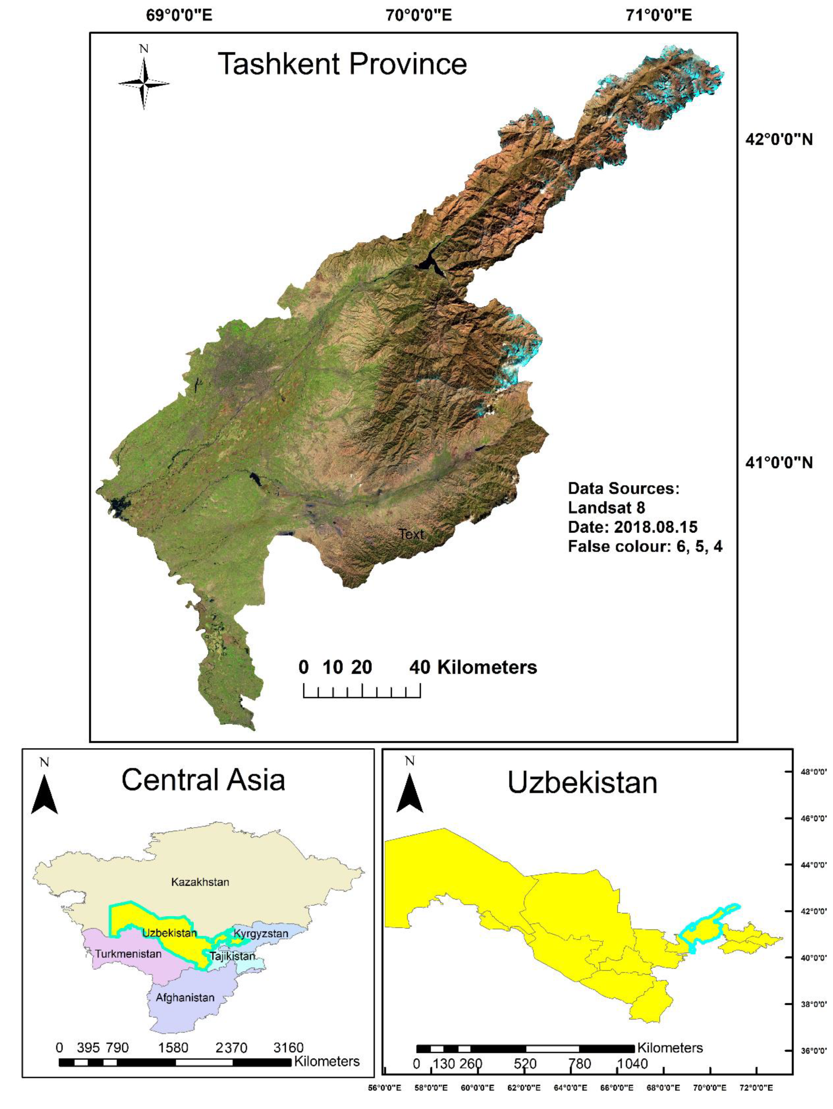
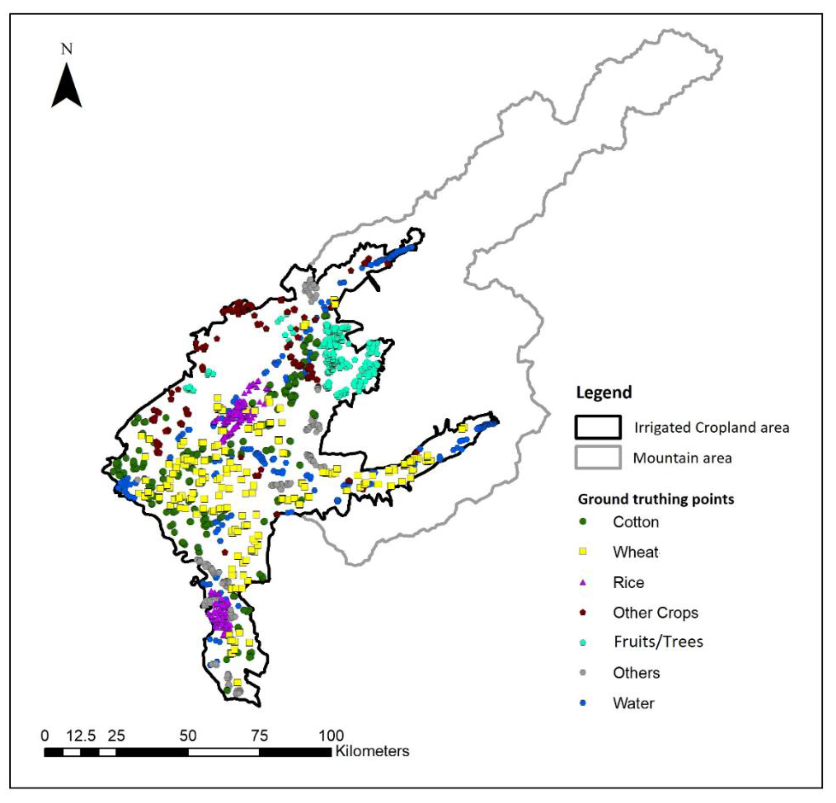
2.1. Study Area
2.2. Data
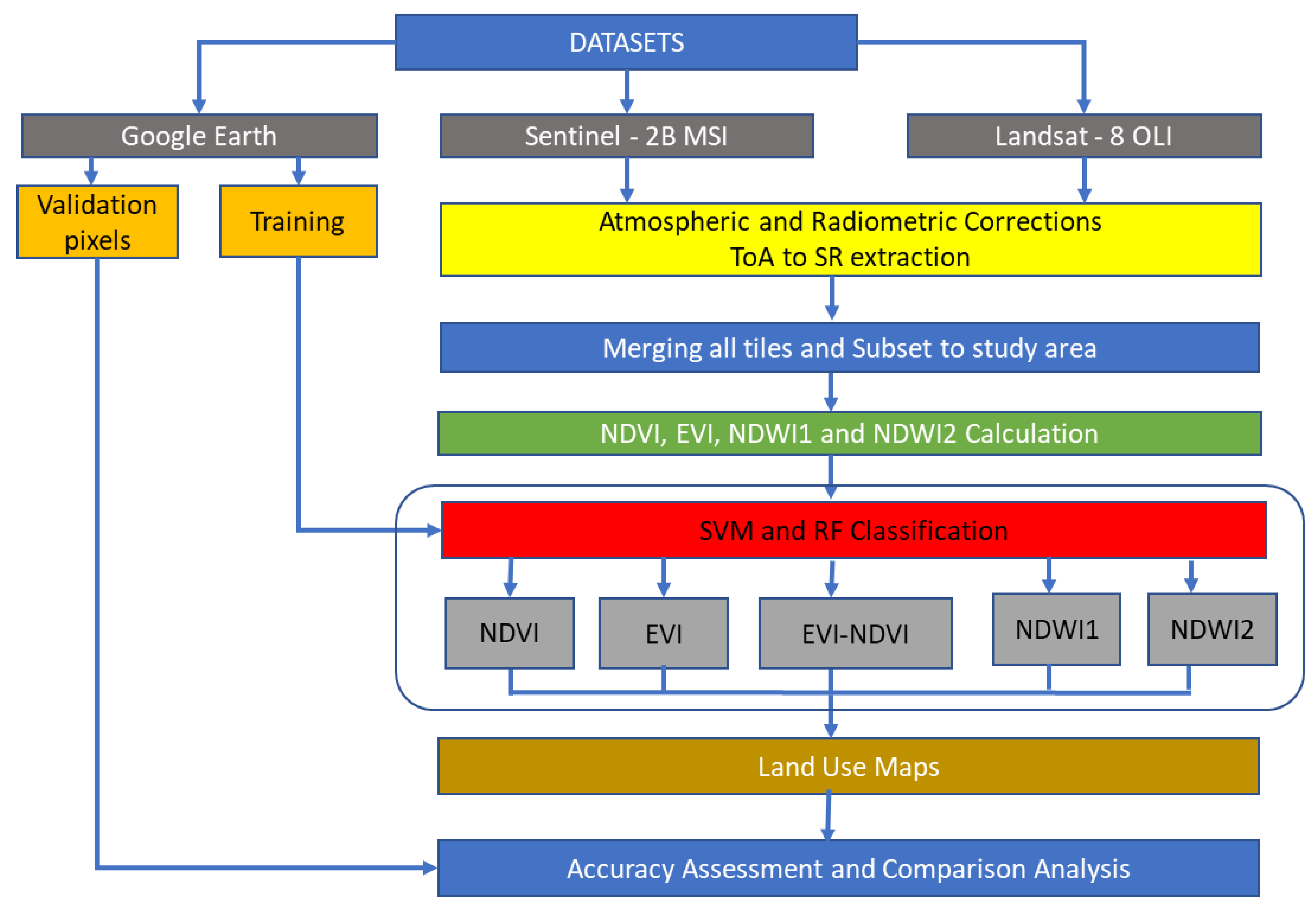
2.3. Methodology
2.3.1. Data Preprocessing
2.3.2. Indexes
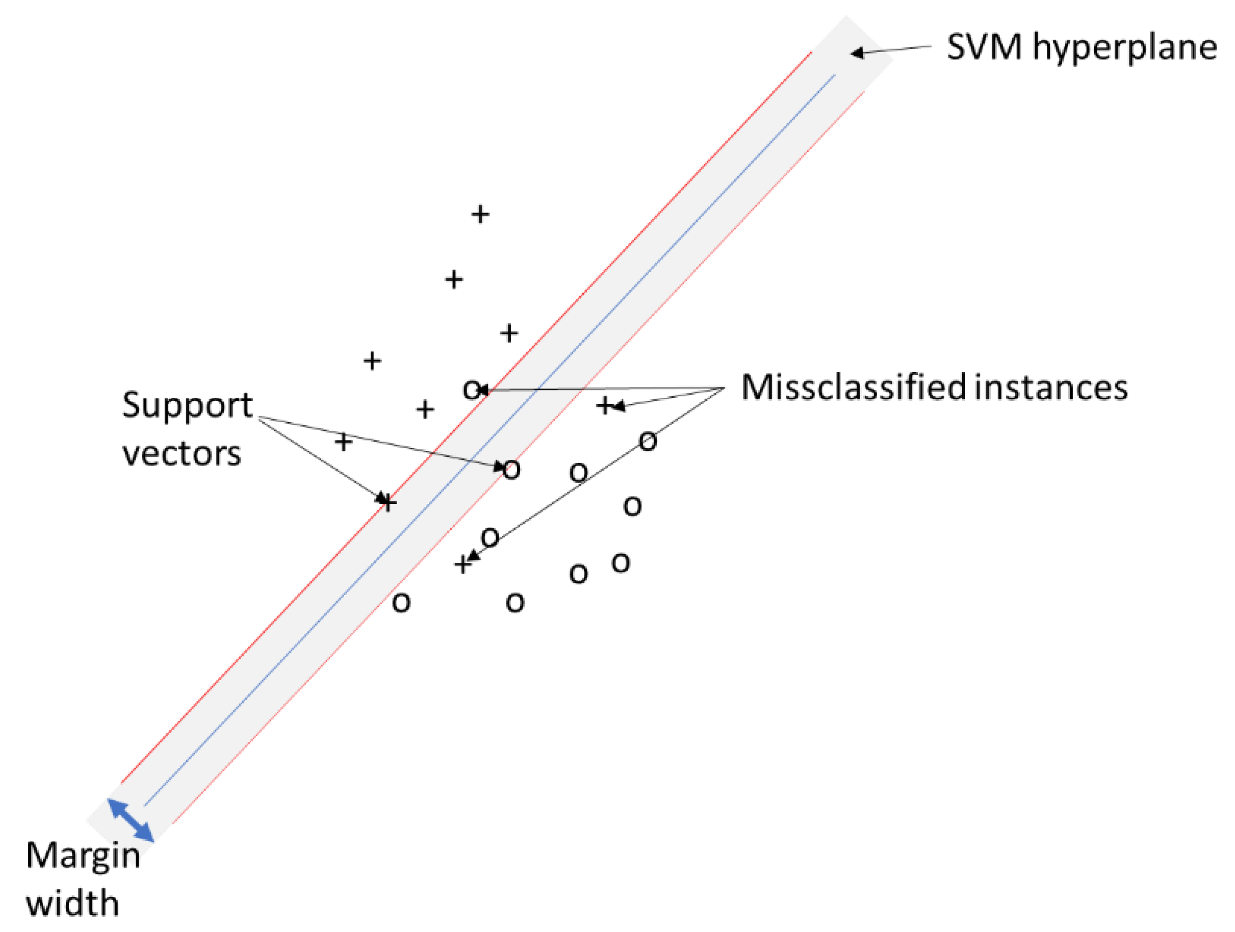
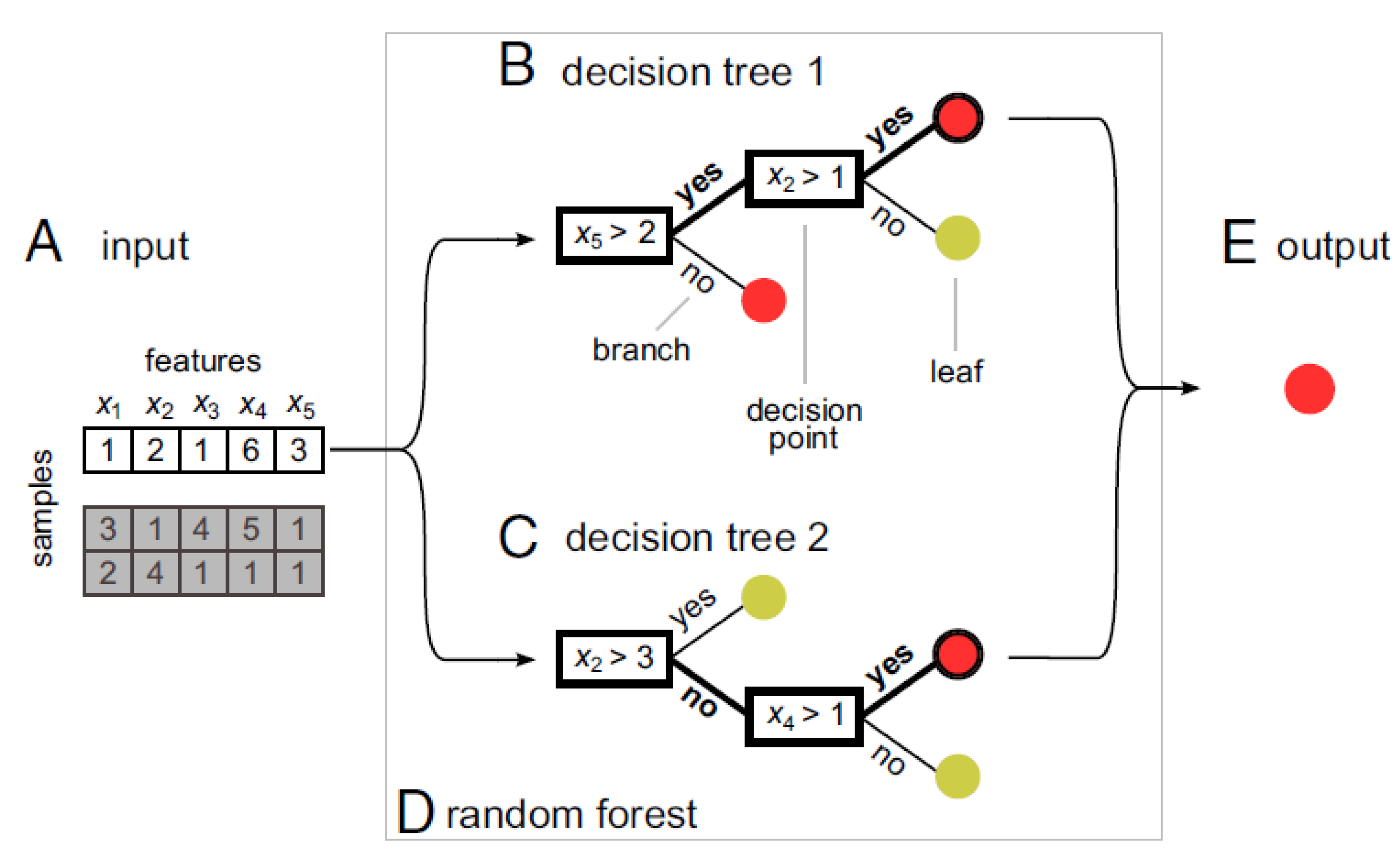
2.3.3. ML Algorithms
2.3.4. Accuracy of RS Classification
3. Results and Discussion
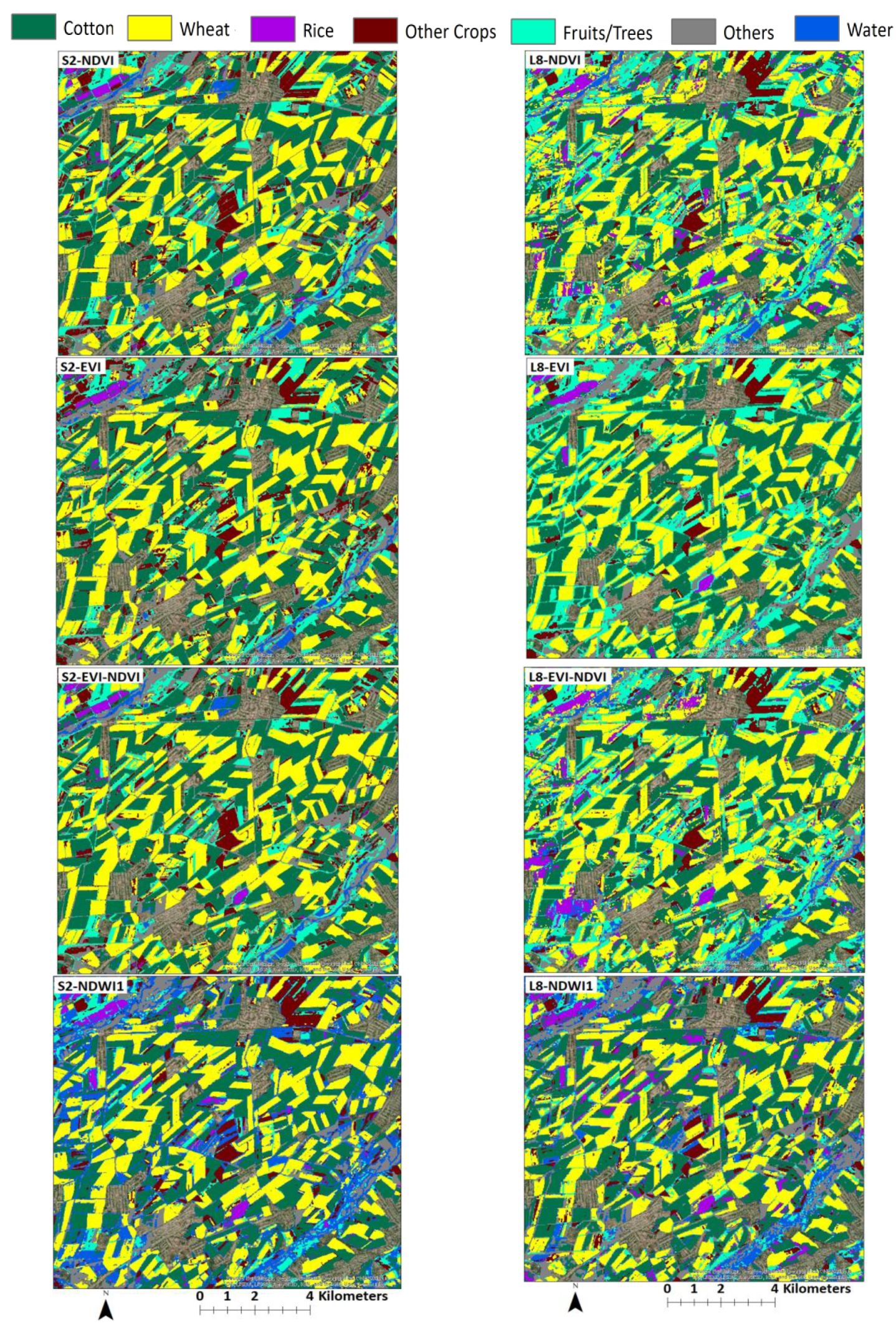
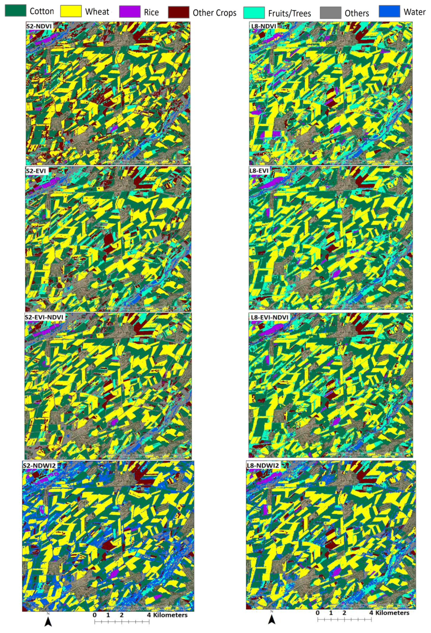
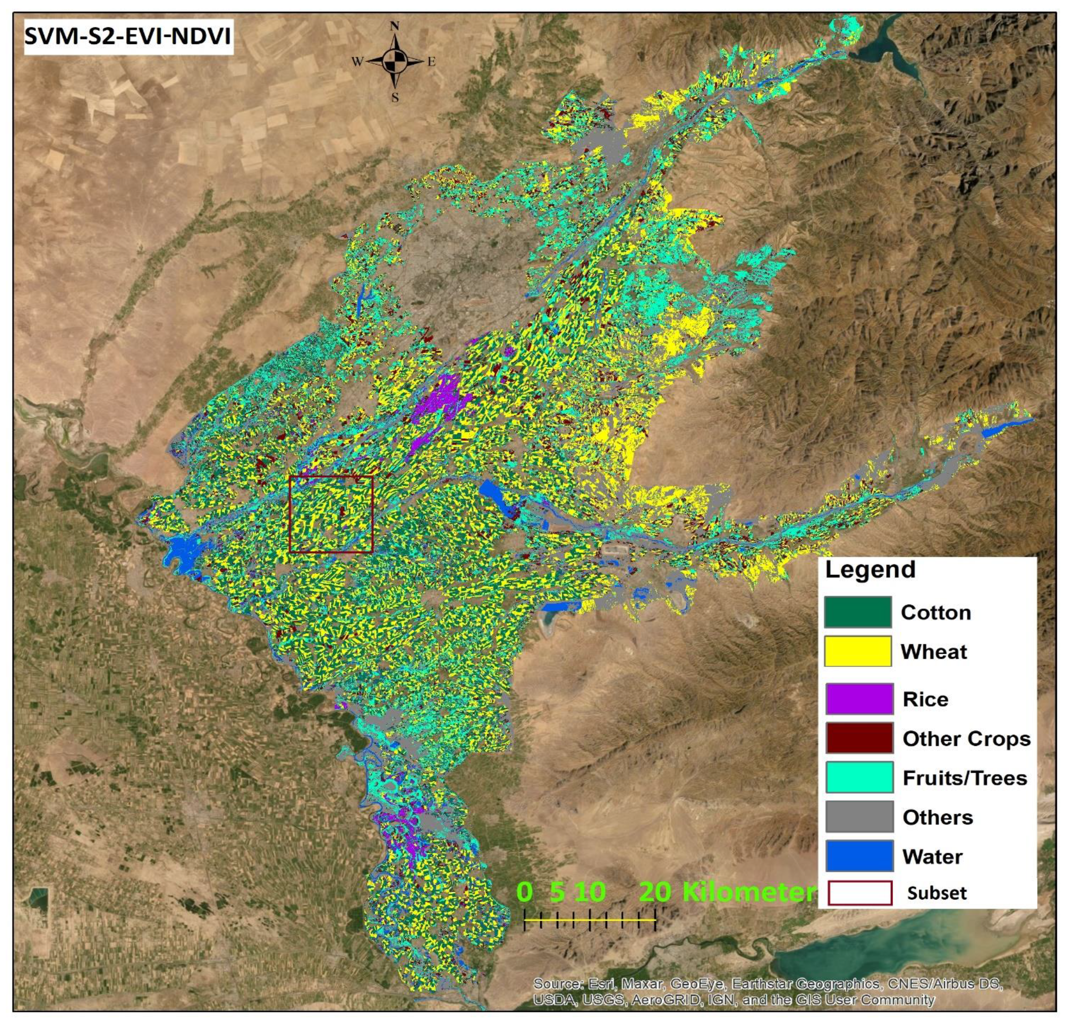
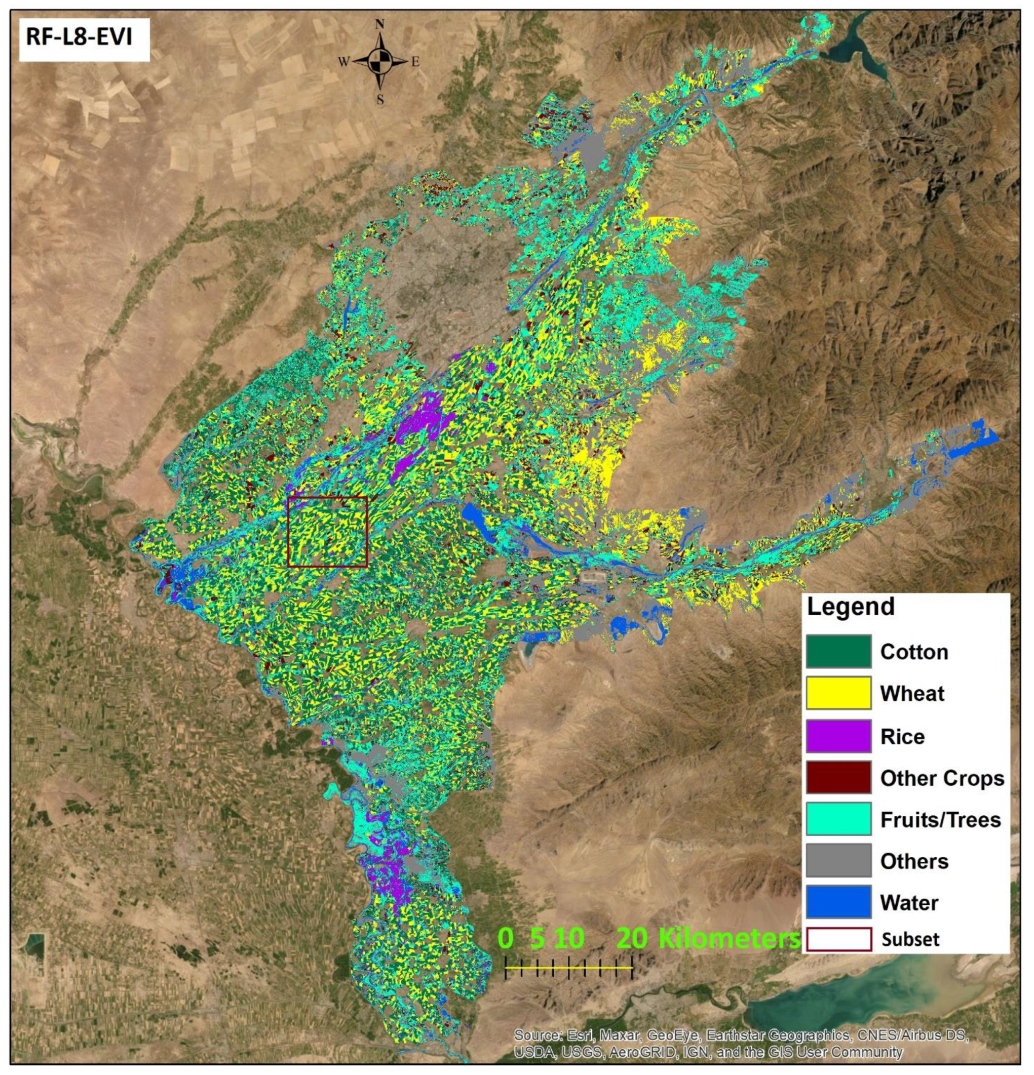
3.1. Results from Land Use Classification
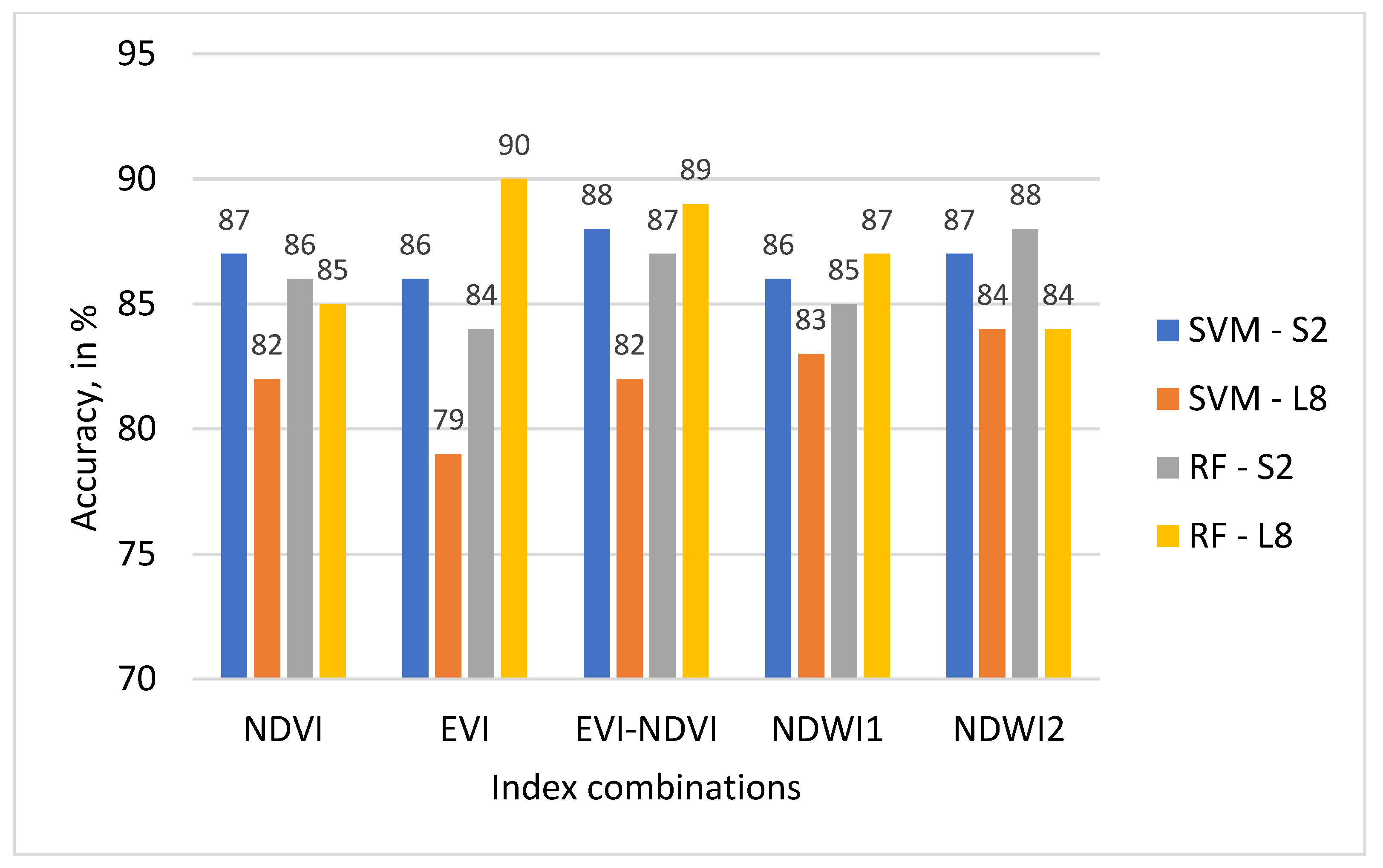
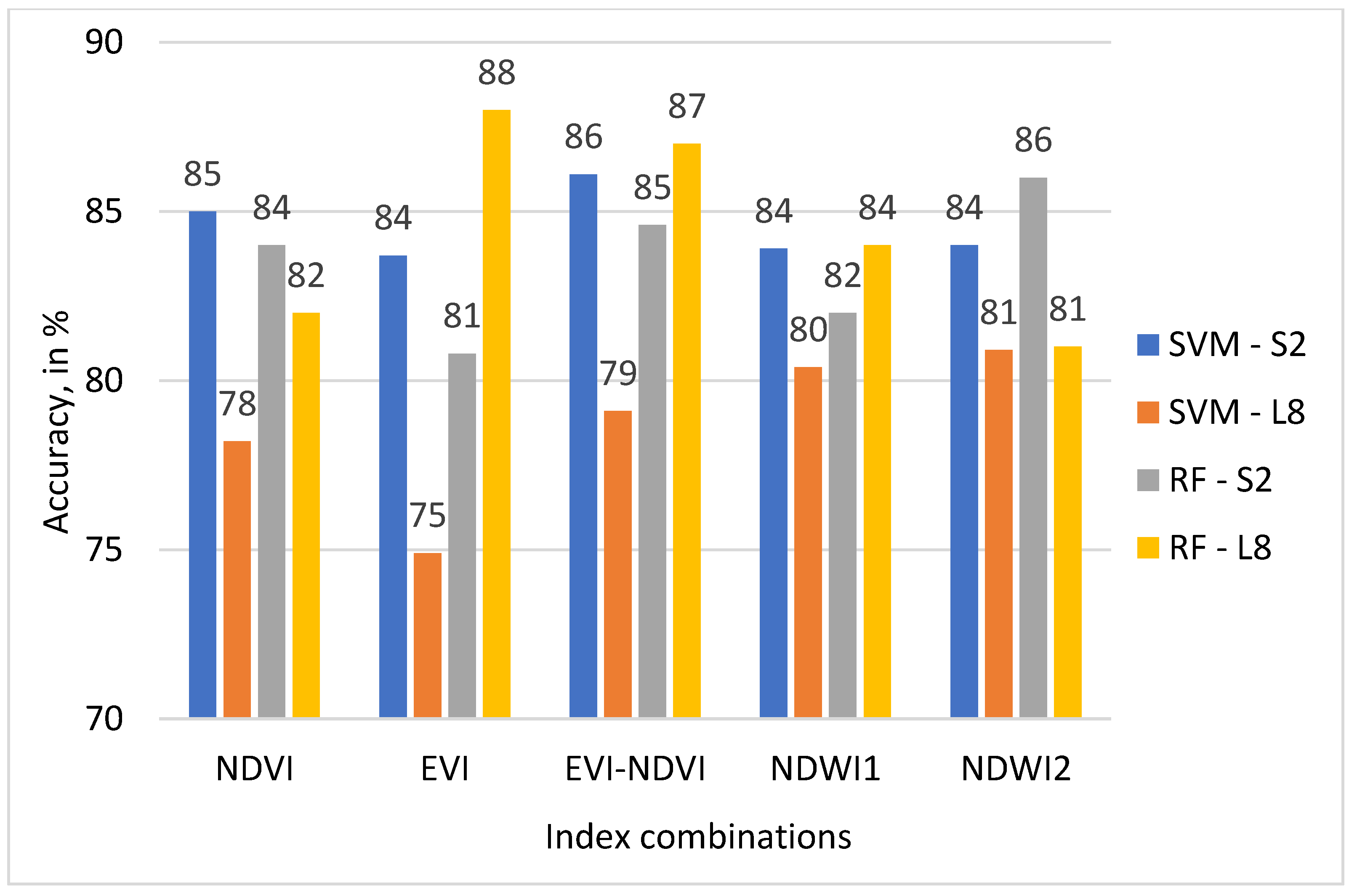
3.2. Classification Accuracy Results
4. Discussion
4.1. Performance of ML Classifiers
4.2. Using Different Indices and Their Performance
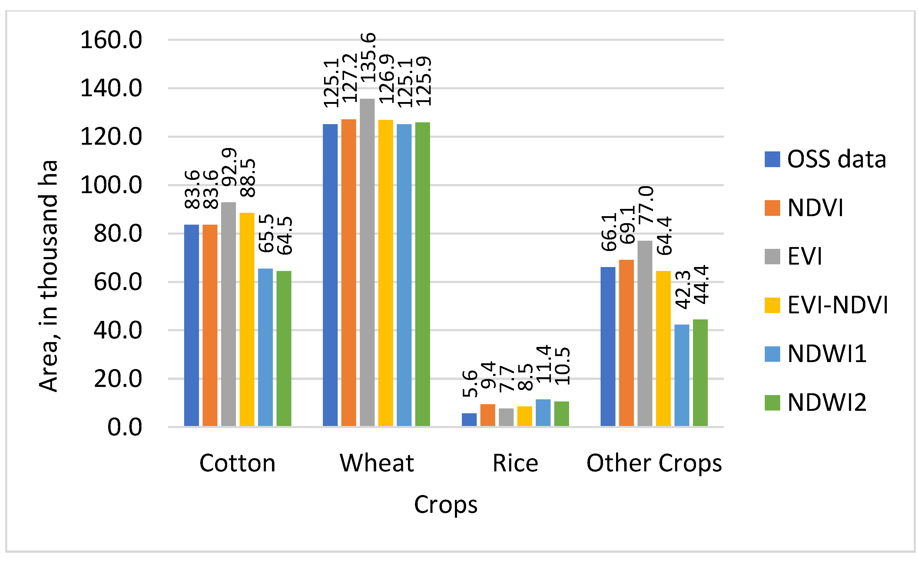
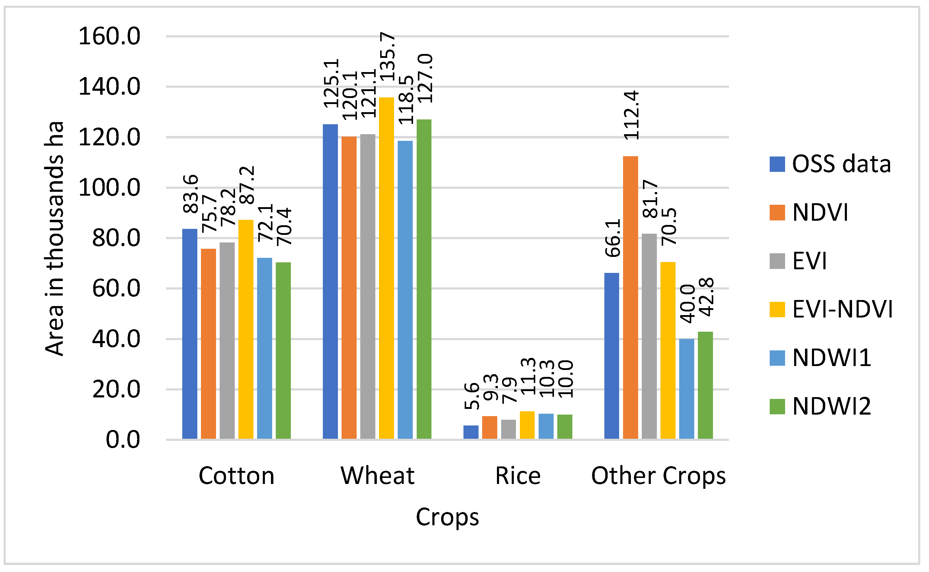
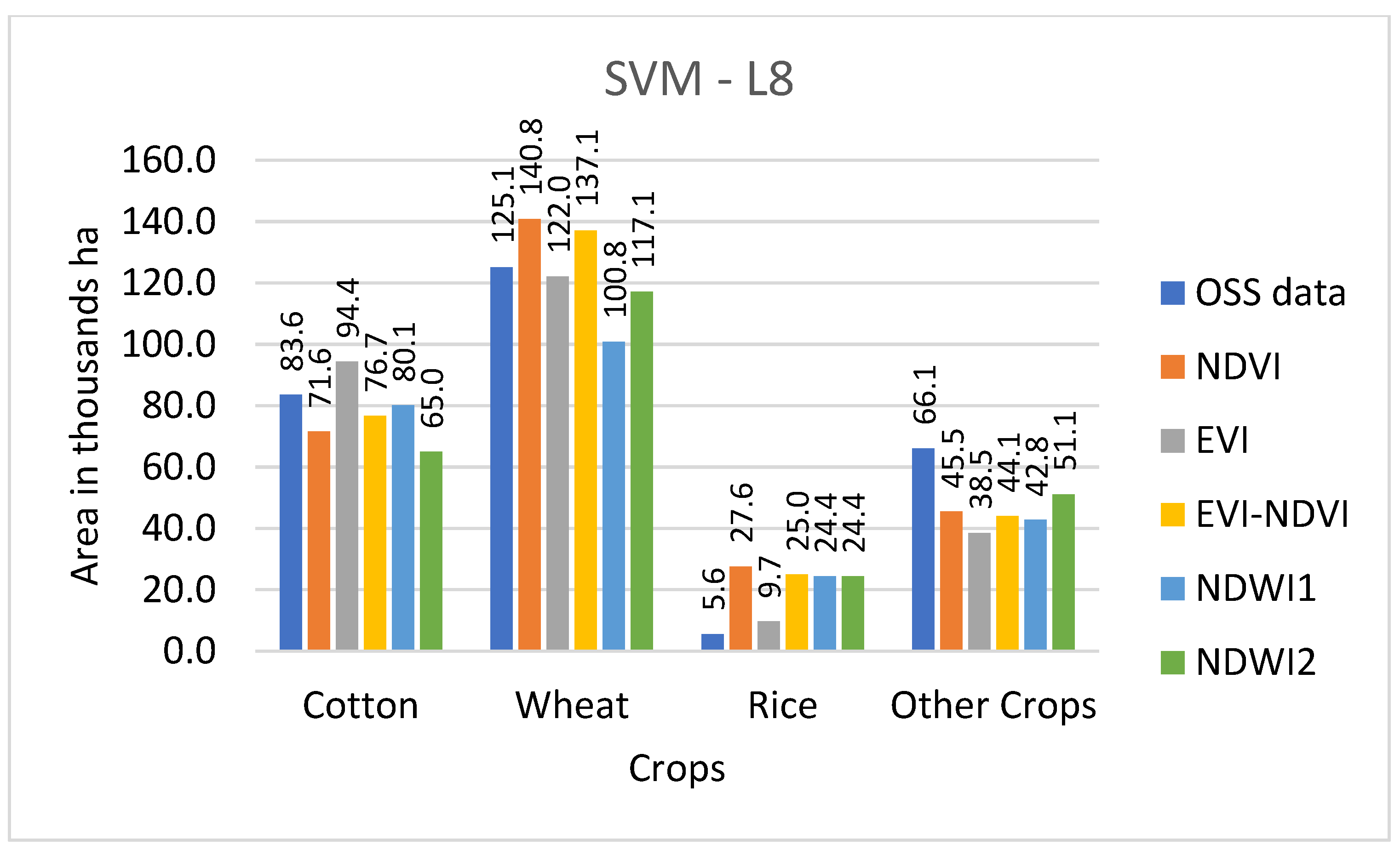
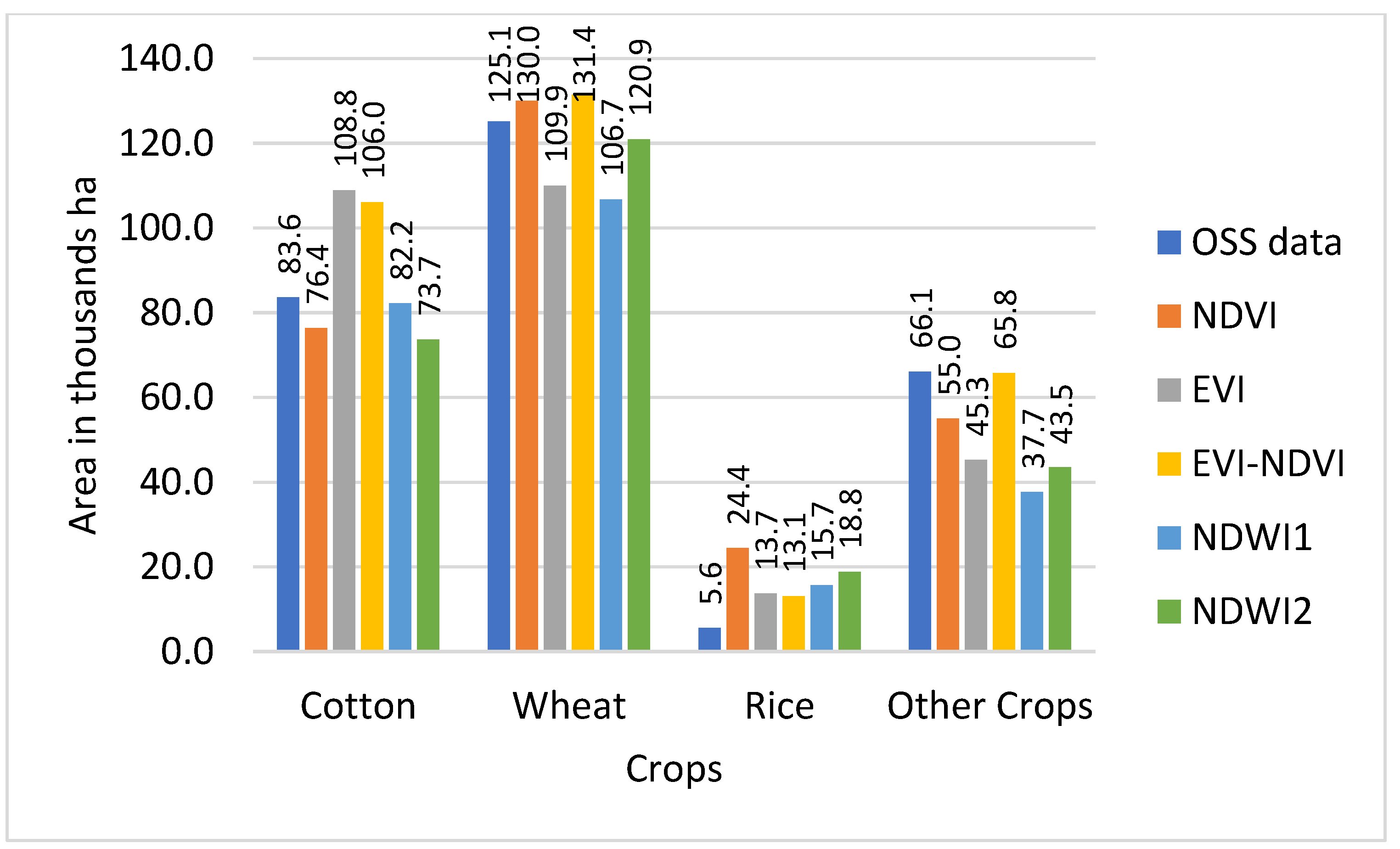
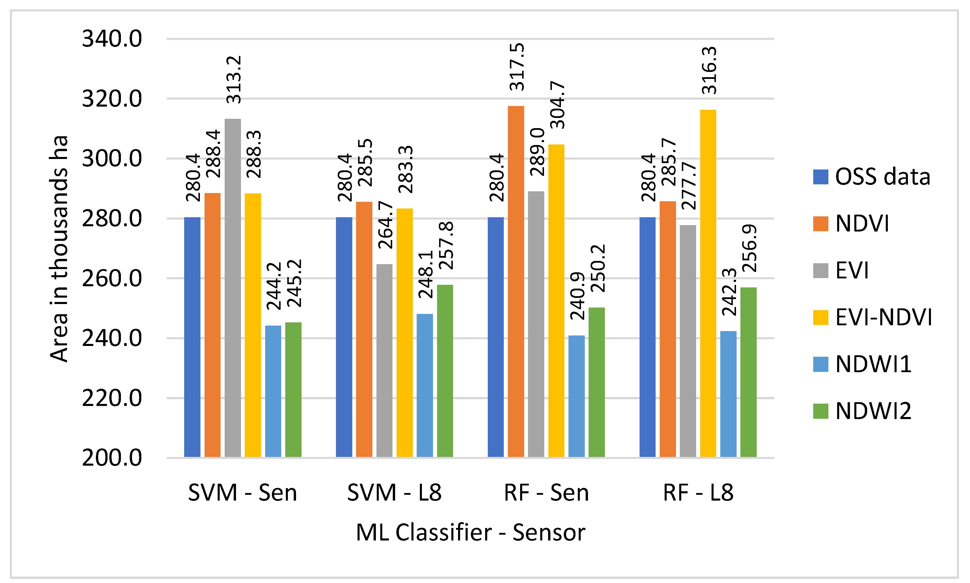
4.3. Comparing Derived Main Crop Types Area with OSS Data
4.4. Theoretical and Practical Implications of the Research
4.5. Limitations and Recommendations
5. Conclusions
Author Contributions
Funding
Institutional Review Board Statement
Informed Consent Statement
Data Availability Statement
Conflicts of Interest
References
- Lambin, E.F.; Geist, H.; Rindfuss, R.R. Introduction: Local processes with global impacts. In Land-Use and Land-Cover Change; Springer: Berlin/Heidelberg, Germany, 2006; pp. 1–8. [Google Scholar]
- Feng, M.; Li, X. Land cover mapping toward finer scales. Sci. Bull. 2020, 65, 1604–1606. [Google Scholar] [CrossRef]
- Wulder, M.A.; Loveland, T.R.; Roy, D.P.; Crawford, C.J.; Masek, J.G.; Woodcock, C.E.; Allen, R.G.; Anderson, M.C.; Belward, A.S.; Cohen, W.B. Current status of Landsat program, science, and applications. Remote Sens. Environ. 2019, 225, 127–147. [Google Scholar] [CrossRef]
- García-Montero, L.G.; Pascual, C.; Martín-Fernández, S.; Sanchez-Paus Díaz, A.; Patriarca, C.; Martín-Ortega, P.; Mollicone, D. Medium-(MR) and Very-High-Resolution (VHR) Image Integration through Collect Earth for Monitoring Forests and Land-Use Changes: Global Forest Survey (GFS) in the Temperate FAO Ecozone in Europe (2000–2015). Remote Sens. 2021, 13, 4344. [Google Scholar] [CrossRef]
- Stephenson, P. Technological advances in biodiversity monitoring: Applicability, opportunities and challenges. Curr. Opin. Environ. Sustain. 2020, 45, 36–41. [Google Scholar] [CrossRef]
- Cavender-Bares, J.; Gamon, J.A.; Townsend, P.A. The use of remote sensing to enhance biodiversity monitoring and detection: A critical challenge for the twenty-first century. In Remote Sensing of Plant Biodiversity; Springer: Cham, Switzerland, 2020; pp. 1–12. [Google Scholar]
- Zaragozí, B.; Giménez-Font, P.; Belda-Antolí, A.; Ramón-Morte, A. A graph-based analysis for generating geographical context from a historical cadastre in Spain (17th and 18th centuries). Hist. Methods: A J. Quant. Interdiscip. Hist. 2019, 52, 228–243. [Google Scholar] [CrossRef]
- Polat, Z.A. Evolution and future trends in global research on cadastre: A bibliometric analysis. GeoJournal 2019, 84, 1121–1134. [Google Scholar] [CrossRef]
- Schmidt-Traub, G. National climate and biodiversity strategies are hamstrung by a lack of maps. Nat. Ecol. Evol. 2021, 5, 1325–1327. [Google Scholar] [CrossRef]
- Karthikeyan, L.; Chawla, I.; Mishra, A.K. A review of remote sensing applications in agriculture for food security: Crop growth and yield, irrigation, and crop losses. J. Hydrol. 2020, 586, 124905. [Google Scholar] [CrossRef]
- Weiss, M.; Jacob, F.; Duveiller, G. Remote sensing for agricultural applications: A meta-review. Remote Sens. Environ. 2020, 236, 111402. [Google Scholar] [CrossRef]
- García-Berná, J.A.; Ouhbi, S.; Benmouna, B.; Garcia-Mateos, G.; Fernández-Alemán, J.L.; Molina-Martínez, J.M. Systematic mapping study on remote sensing in agriculture. Appl. Sci. 2020, 10, 3456. [Google Scholar] [CrossRef]
- FAO. World Food Situation. Food and Agriculture Organziation of the United Nations. 2019. Available online: http://www.fao.org/worldfoodsituation/csdb/en/ (accessed on 15 March 2020).
- Habibie, M.I.; Noguchi, R.; Shusuke, M.; Ahamed, T. Land suitability analysis for maize production in Indonesia using satellite remote sensing and GIS-based multicriteria decision support system. GeoJournal 2021, 86, 777–807. [Google Scholar] [CrossRef]
- Zhang, L.; Liu, Z.; Ren, T.; Liu, D.; Ma, Z.; Tong, L.; Zhang, C.; Zhou, T.; Zhang, X.; Li, S. Identification of seed maize fields with high spatial resolution and multiple spectral remote sensing using random forest classifier. Remote Sens. 2020, 12, 362. [Google Scholar] [CrossRef] [Green Version]
- Ahmad, I.; Singh, A.; Fahad, M.; Waqas, M.M. Remote sensing-based framework to predict and assess the interannual variability of maize yields in Pakistan using Landsat imagery. Comput. Electron. Agric. 2020, 178, 105732. [Google Scholar] [CrossRef]
- Chen, X.; Wang, W.; Chen, J.; Zhu, X.; Shen, M.; Gan, L.; Cao, X. Does any phenological event defined by remote sensing deserve particular attention? An examination of spring phenology of winter wheat in Northern China. Ecol. Indic. 2020, 116, 106456. [Google Scholar] [CrossRef]
- Wang, S.; Chen, J.; Rao, Y.; Liu, L.; Wang, W.; Dong, Q. Response of winter wheat to spring frost from a remote sensing perspective: Damage estimation and influential factors. ISPRS J. Photogramm. Remote Sens. 2020, 168, 221–235. [Google Scholar] [CrossRef]
- dela Torre, D.M.G.; Gao, J.; Macinnis-Ng, C. Remote sensing-based estimation of rice yields using various models: A critical review. Geo-Spat. Inf. Sci. 2021, 24, 580–603. [Google Scholar] [CrossRef]
- Chuvieco, E. Fundamentals of Satellite Remote Sensing: An Environmental Approach; CRC Press: Boca Raton, FL, USA, 2020. [Google Scholar]
- CIA. Uzbekistan. Central Intelligence Agency. 2021. Available online: https://www.cia.gov/the-world-factbook/countries/uzbekistan/ (accessed on 14 November 2021).
- Erdanaev, E.; Kappas, M.; Pulatov, A.; Klinge, M. Short Review of Climate and Land Use change Impact on Land Degradation in Tashkent Province. Int. J. Geoinf. 2015, 11, 39–48. [Google Scholar]
- UzGosKomStat. Agriculture of Uzbekistan, and Official Figures on Structure of Individual Farms by Production Specialization across Provinces; The State Committee of Statistics of Uzbekistan: Tashkent, Uzbekistan, 2019. [Google Scholar]
- USGS. Earth Explorer. United States Geological Survey. 2020. Available online: https://earthexplorer.usgs.gov/ (accessed on 16 March 2020).
- ESA. Sentinel 2 Product Specification Document; European Space Agency: Paris, France, 2021; Available online: https://sentinel.esa.int/documents/247904/685211/Sentinel-2-Products-Specification-Document (accessed on 16 March 2020).
- USGS. Landsat 8. United States Geological Survey. 2020. Available online: https://www.usgs.gov/core-science-systems/nli/landsat/landsat-8?qt-science_support_page_related_con=0#qt-science_support_page_related_con (accessed on 16 March 2020).
- Erdanaev, E.; Kappas, M.; Wyss, D. The Identification of Irrigated Crop Types Using Support Vector Machine, Random Forest and Maximum Likelihood Classification Methods with Sentinel-2 Data in 2018: Tashkent Province, Uzbekistan. Int. J. Geoinf. 2022, 18, 37–53. [Google Scholar] [CrossRef]
- Clemente, J.P.; Fontanelli, G.; Ovando, G.G.; Roa, Y.L.B.; Lapini, A.; Santi, E. Google Earth Engine: Application of Algorithms For Remote Sensing of Crops in Tuscany (Italy). Int. Arch. Photogramm. Remote Sens. Spatial Inf. Sci. 2020, XLII-3/W12-2020, 291–296. [Google Scholar] [CrossRef]
- Rouse, J.W.; Haas, R.H.; Schell, J.A.; Deering, D.W. Monitoring vegetation systems in the Great Plains with ERTS. NASA Spec. Publ. 1974, 351, 309. [Google Scholar]
- Huete, A.; Justice, C.; Van Leeuwen, W. MODIS vegetation index (MOD13). Algorithm Theor. Basis Doc. 1999, 3, 295–309. [Google Scholar]
- Gao, B.-C. Normalized difference water index for remote sensing of vegetation liquid water from space. Imaging Spectrom. 1995, 2480, 877. [Google Scholar]
- Vapnik, V. Estimation of Dependences based on Empirical Data; Springer Science & Business Media: Berlin/Heidelberg, Germany, 1982. [Google Scholar]
- Zhu, G.; Blumberg, D.G. Classification using ASTER data and SVM algorithms: The case study of Beer Sheva, Israel. Remote Sens. Environ. 2002, 80, 233–240. [Google Scholar] [CrossRef]
- Burges, C.J. A tutorial on support vector machines for pattern recognition. Data Min. Knowl. Discov. 1998, 2, 121–167. [Google Scholar] [CrossRef]
- Breiman, L. Random forests. Mach. Learn. 2001, 45, 5–32. [Google Scholar] [CrossRef] [Green Version]
- Pal, M. Random forest classifier for remote sensing classification. Int. J. Remote Sens. 2007, 26, 217–222. [Google Scholar] [CrossRef]
- Denisko, D.; Hoffman, M.M. Classification and interaction in random forests. Proc. Natl. Acad. Sci. USA 2018, 115, 1690–1692. [Google Scholar] [CrossRef] [Green Version]
- Thanh Noi, P.; Kappas, M. Comparison of Random Forest, k-Nearest Neighbor, and Support Vector Machine Classifiers for Land Cover Classification Using Sentinel-2 Imagery. Sensors 2018, 18, 18. [Google Scholar] [CrossRef] [PubMed] [Green Version]
- Nitze, I.; Schulthess, U.; Asche, C. Comparison of Machine Learning Algorithms Random Forest, Artificial Neural Network and Support Vector Machine to Maximum Likelihood for Supervised Crop Type Classification. In Proceedings of the The 4th International Conference on GEographic Object Based Image Analysis (Geobia), Rio de Janeiro, Brazil, 7–9 May 2012. [Google Scholar]
- Congalton, R.C. A Review of Assessing the Accuracy of Classifications of Remotely Sensed Data. Remote Sens. Environ. 1991, 37, 35–46. [Google Scholar] [CrossRef]
- Basukala, A.K.; Oldenburg, C.; Schellberg, J.; Sultanov, M.; Dubovyk, O. Towards improved land use mapping of irrigated croplands: Performance assessment of different image classification algorithms and approaches. Eur. J. Remote Sens. 2017, 50, 187–201. [Google Scholar] [CrossRef] [Green Version]
- Saini, R.; Ghosh, S.K. Crop Classification on Single Date Sentinel-2 Imagery Using Random Forest and Suppor Vector Machine. ISPRS Int. Arch. Photogramm. Remote Sens. Spat. Inf. Sci. 2018, XLII-5, 683–688. [Google Scholar] [CrossRef] [Green Version]
- Virnodkar, S.; Pachghare, V.K.; Patil, V.C.; Jha, S.K. Performance Evaluation of RF and SVM for Sugarcane Classification Using Sentinel-2 NDVI Time-Series. In Progress in Advanced Computing and Intelligent Engineering; Panigrahi, C.R., Pati, B., Mohapatra, P., Buyya, R., Li, K., Eds.; Advances in Intelligent Systems and Computing; Springer: Singapore, 2021; Volume 1199, pp. 163–174. [Google Scholar]
- Azeez, N.; Yahya, W.; Al-Taie, I.; Basbrain, A.; Clark, A. Regional Agricultural Land Classification Based on Random Forest (RF), Decision Tree, and SVMs Techniques. In Fourth International Congress on Information and Communication Technology: ICICT 2019, London. Volume 1/Xin-She Yang, Simon Sherratt, Nilanjan Dey, Amit Joshi, editors; Yang, X.-S., Sherratt, S., Dey, N., Joshi, A., Eds.; Springer: Singapore, 2020; pp. 73–81. ISBN 978-981-15-0636-9. [Google Scholar]
- Bofana, J.; Zhang, M.; Nabil, M.; Wu, B.; Tian, F.; Liu, W.; Zeng, H.; Zhang, N.; Nangombe, S.; Cipriano, S.; et al. Comparison of Different Cropland Classification Methods under Diversified Agroecological Conditions in the Zambezi River Basin. Remote Sens. 2020, 12, 2096. [Google Scholar] [CrossRef]
- Kobayashi, N.; Tani, H.; Wang, X.; Sonobe, R. Crop classification using spectral indices derived from Sentinel-2A imagery. J. Inf. Telecommun. 2020, 4, 67–90. [Google Scholar] [CrossRef]
- Palchowdhuri, Y.; Valcarce-Diñeiro, R.; King, P.; Sanabria-Soto, M. Classification of multi-temporal spectral indices for crop type mapping: A case study in Coalville, UK. J. Agric. Sci. 2018, 156, 24–36. [Google Scholar] [CrossRef]
- Sonobe, R.; Yamaya, Y.; Tani, H.; Wang, X.; Kobayashi, N.; Mochizuki, K.-I. Crop classification from Sentinel-2-derived vegetation indices using ensemble learning. J. Appl. Remote Sens. 2018, 12, 026019. [Google Scholar] [CrossRef] [Green Version]
- Wardlow, B.D.; Egbert, S.L. A comparison of MODIS 250-m EVI and NDVI data for crop mapping: A case study for southwest Kansas. Int. J. Remote Sens. 2010, 31, 805–830. [Google Scholar] [CrossRef]
- Hao, P.-Y.; Tang, H.-J.; Chen, Z.-X.; Meng, Q.-Y.; Kang, Y.-P. Early-season crop type mapping using 30-m reference time series. J. Integr. Agric. 2020, 19, 1897–1911. [Google Scholar] [CrossRef]
- Pan, L.; Xia, H.; Zhao, X.; Guo, Y.; Qin, Y. Mapping Winter Crops Using a Phenology Algorithm, Time-Series Sentinel-2 and Landsat-7/8 Images, and Google Earth Engine. Remote Sens. 2021, 13, 2510. [Google Scholar] [CrossRef]
- Demarez, V.; Helen, F.; Marais-Sicre, C.; Baup, F. In-Season Mapping of Irrigated Crops Using Landsat 8 and Sentinel-1 Time Series. Remote Sens. 2019, 11, 118. [Google Scholar] [CrossRef] [Green Version]
- Vuolo, F.; Neuwirth, M.; Immitzer, M.; Atzberger, C.; Ng, W.-T. How much does multi-temporal Sentinel-2 data improve crop type classification? Int. J. Appl. Earth Obs. Geoinf. 2018, 72, 122–130. [Google Scholar] [CrossRef]
- Yi, Z.; Jia, L.; Chen, Q. Crop Classification Using Multi-Temporal Sentinel-2 Data in the Shiyang River Basin of China. Remote Sens. 2020, 12, 4052. [Google Scholar] [CrossRef]
- Song, X.-P.; Huang, W.; Hansen, M.C.; Potapov, P. An evaluation of Landsat, Sentinel-2, Sentinel-1 and MODIS data for crop type mapping. Sci. Remote Sens. 2021, 3, 100018. [Google Scholar] [CrossRef]
- Gerts, J.; Juliev, M.; Pulatov, A. Multi-temporal monitoring of cotton growth through the vegetation profile classification for Tashkent province, Uzbekistan. GeoScape 2020, 14, 62–69. [Google Scholar] [CrossRef]
- Oliphant, A.J.; Thenkabail, P.S.; Teluguntla, P.; Xiong, J.; Gumma, M.K.; Congalton, R.G.; Yadav, K. Mapping cropland extent of Southeast and Northeast Asia using multi-year time-series Landsat 30-m data using a random forest classifier on the Google Earth Engine cloud. Int. J. Appl. Earth Observ. Geoinf. 2019, 81, 110–124. [Google Scholar] [CrossRef]
- Asam, S.; Gessner, U.; González, R.A.; Wenzl, M.; Kriese, J.; Kuenzer, C. Mapping Crop Types of Germany by Combining Temporal Statistical Metrics of Sentinel-1 and Sentinel-2 Time Series with LPIS Data. Remote Sens. 2022, 14, 2981. [Google Scholar] [CrossRef]


| Month | S2 Multispectral Imaging (MSI) Date | L8 Operation Land Imager (OLI) Date | |||||
|---|---|---|---|---|---|---|---|
| T42TVL | T42TWK | T42TWL | T42TWM | 153/031 | 154/031 | 154/032 | |
| May | 25 | 7 | 7 | 7 | 28 | 3 | 3 |
| June | 24 | 6 | 6 | 6 | 13 | 20 | 20 |
| July | 9 | 1 | 1 | 1 | 15 | 22 | 22 |
| August | 3 | 5 | 5 | 5 | 16 | 7 | 7 |
| September | 2 | 4 | 4 | 4 | 1 | 8 | 8 |
| October | 2 | 4 | 4 | 4 | 3 | 26 | 26 |
| Band Number | S2 MSI | L8 OLI | ||||
|---|---|---|---|---|---|---|
| Description | Wave-Lengths (nm) | Spatial Resolution (m) | Description | Wave-Lengths (nm) | Spatial Resolution (m) | |
| 1 | Coastal aerosol | 433–453 | 60 | Coastal aerosol | 433–453 | 30 |
| 2 | Blue | 458–523 | 10 | Blue | 450–515 | 30 |
| 3 | Green | 543–578 | 10 | Green | 525–600 | 30 |
| 4 | Red | 650–680 | 10 | Red | 630–680 | 30 |
| 5 | Vegetation Red Edge 1 | 698–713 | 20 | NIR | 845–885 | 30 |
| 6 | Vegetation Red Edge 2 | 733–748 | 20 | SWIR 1 | 1570–1650 | 30 |
| 7 | Vegetation Red Edge 3 | 773–793 | 20 | SWIR 2 | 2100–2300 | 30 |
| 8 | Near-Infrared (NIR) | 785–900 | 10 | Panchromatic | 500–680 | 15 |
| 8a | Narrow NIR | 855–875 | 20 | |||
| 9 | Water vapor | 935–955 | 60 | Cirrus | 1360–1390 | 30 |
| 10 | SWIR-Cirrus | 1360–1390 | 60 | Thermal Infrared (TIRS) 1 | 10,600–11,200 | 100 |
| 11 | SWIR 1 | 1565–1655 | 20 | Thermal Infrared (TIRS) 2 | 11,500–12,500 | 100 |
| 12 | SWIR 2 | 2100–2280 | 20 | |||
| Land Use | Training (Polygons/Pixels) | Validation (Pixels) |
|---|---|---|
| Cotton | 150/2528 | 250 |
| Wheat | 300/5750 | 500 |
| Rice | 150/3038 | 250 |
| Other Crops | 150/2248 | 250 |
| Fruits/Trees | 150/3642 | 250 |
| Bare land | 150/2560 | 250 |
| Others | 150/2601 | 250 |
| Water | 150/2899 | 250 |
| S2-SVM | ||||||
| NDVI | EVI | EVI-NDVI | NDWI1 | NDWI2 | ||
| Cotton | 0 | −9.3 | −4.9 | 18.1 | 19.1 | |
| Wheat | −2.1 | −10.5 | −1.8 | 0 | −0.8 | |
| Rice | −3.8 | −2.1 | −2.9 | −5.8 | −4.9 | |
| Other crops | −3 | −10.9 | 1.7 | 23.8 | 21.7 | |
| AM | −2.2 | −8.2 | −2.0 | 9.0 | 8.8 | |
| WA (OSS): | −0.4 | −2.5 | −0.5 | 2.7 | 2.6 | |
| S2-RF | ||||||
| NDVI | EVI | EVI-NDVI | NDWI1 | NDWI2 | ||
| Cotton | 7.9 | 5.4 | −3.6 | 11.5 | 13.2 | |
| Wheat | 5 | 4 | −10.6 | 6.6 | −1.9 | |
| Rice | −3.7 | −2.3 | −5.7 | −4.7 | −4.4 | |
| Other crops | −46.3 | −15.6 | −4.4 | 26.1 | 23.3 | |
| AM | −9.3 | −2.1 | −6.1 | 9.9 | 7.6 | |
| WA (OSS): | −1.6 | −0.1 | −1.7 | 31 | 2.1 | |
| L8-SVM | ||||||
| NDVI | EVI | EVI-NDVI | NDWI1 | NDWI2 | ||
| Cotton | 12 | 12 | −10.8 | 6.9 | 3.5 | |
| Wheat | −15.7 | −15.7 | 3.1 | −12 | 24.3 | |
| Rice | −22 | −4.1 | −19.4 | −18.8 | −18.8 | |
| Other crops | 20.6 | 27.6 | 22 | 23.3 | 15 | |
| AM | −1.3 | 4.9 | −1.3 | −0.2 | 6.0 | |
| WA (OSS): | 0.2 | 0.7 | 0.7 | 0.5 | 3.8 | |
| L8-RF | ||||||
| NDVI | EVI | EVI-NDVI | NDWI1 | NDWI2 | ||
| Cotton | 7.2 | 7.2 | −25.2 | −22.4 | 1.4 | |
| Wheat | −4.9 | −4.9 | 15.2 | −6.3 | 19 | |
| Rice | −18.8 | −8.1 | −7.5 | −10.1 | −13.2 | |
| Other crops | −1.4 | 3.8 | −4.3 | −2.6 | 7.5 | |
| AM | −1.35 | 3.75 | −4.3 | −2.6 | 7.45 | |
| WA (OSS): | 0.6 | 1.2 | −0.2 | −0.7 | 3.5 | |
| Classes | NDVI | EVI | EVI-NDVI | NDWI1 | NDWI2 | |||||||||||||||
|---|---|---|---|---|---|---|---|---|---|---|---|---|---|---|---|---|---|---|---|---|
| UA | PA | UA | PA | UA | PA | UA | PA | UA | PA | |||||||||||
| S2 | L8 | S2 | L8 | S2 | L8 | S2 | L8 | S2 | L8 | S2 | L8 | S2 | L8 | S2 | L8 | S2 | L8 | S2 | L8 | |
| Cotton | 84 | 75 | 94 | 73 | 74 | 85 | 96 | 92 | 87 | 78 | 97 | 81 | 93 | 86 | 92 | 82 | 90 | 90 | 90 | 85 |
| Wheat | 87 | 85 | 92 | 81 | 86 | 78 | 92 | 89 | 88 | 82 | 91 | 83 | 92 | 93 | 93 | 90 | 95 | 89 | 91 | 89 |
| Rice | 93 | 75 | 78 | 68 | 97 | 94 | 70 | 94 | 95 | 83 | 80 | 74 | 90 | 83 | 92 | 85 | 92 | 84 | 88 | 87 |
| Other crops | 76 | 79 | 80 | 86 | 84 | 86 | 80 | 60 | 78 | 78 | 80 | 76 | 87 | 80 | 86 | 72 | 84 | 78 | 89 | 72 |
| Fruits/trees | 87 | 81 | 88 | 89 | 81 | 69 | 87 | 88 | 86 | 81 | 89 | 88 | 71 | 76 | 78 | 80 | 73 | 83 | 74 | 81 |
| Others | 89 | 84 | 83 | 85 | 92 | 65 | 75 | 86 | 89 | 91 | 83 | 82 | 92 | 87 | 82 | 90 | 94 | 85 | 86 | 83 |
| Water | 97 | 88 | 95 | 92 | 98 | 99 | 98 | 31 | 98 | 85 | 96 | 93 | 76 | 72 | 75 | 80 | 76 | 74 | 87 | 83 |
| AM | 88 | 81 | 87 | 82 | 87 | 82 | 85 | 77 | 89 | 83 | 88 | 82 | 86 | 82 | 85 | 83 | 86 | 83 | 86 | 83 |
| OA-S2 | 87 | 86 | 88 | 86 | 87 | |||||||||||||||
| OA-L8 | 82 | 79 | 82 | 83 | 84 | |||||||||||||||
| KA-S2 | 85 | 84 | 86 | 84 | 84 | |||||||||||||||
| KA-L8 | 78 | 75 | 79 | 80 | 81 | |||||||||||||||
| Classes | NDVI | EVI | EVI-NDVI | NDWI1 | NDWI2 | |||||||||||||||
|---|---|---|---|---|---|---|---|---|---|---|---|---|---|---|---|---|---|---|---|---|
| UA | PA | UA | PA | UA | PA | UA | PA | UA | PA | |||||||||||
| S2 | L8 | S2 | L8 | S2 | L8 | S2 | L8 | S2 | L8 | S2 | L8 | S2 | L8 | S2 | L8 | S2 | L8 | S2 | L8 | |
| Cotton | 81 | 77 | 91 | 84 | 77 | 88 | 92 | 95 | 77 | 89 | 94 | 95 | 94 | 90 | 95 | 90 | 93 | 90 | 94 | 90 |
| Wheat | 91 | 90 | 87 | 84 | 86 | 94 | 89 | 92 | 91 | 92 | 93 | 87 | 92 | 94 | 92 | 92 | 94 | 89 | 93 | 90 |
| Rice | 94 | 83 | 76 | 76 | 96 | 94 | 68 | 97 | 92 | 94 | 76 | 97 | 90 | 90 | 94 | 88 | 94 | 90 | 93 | 90 |
| Other crops | 72 | 83 | 85 | 84 | 70 | 87 | 78 | 85 | 84 | 76 | 78 | 79 | 88 | 86 | 78 | 77 | 90 | 85 | 84 | 71 |
| Fruits/trees | 82 | 81 | 86 | 89 | 81 | 78 | 85 | 81 | 81 | 85 | 81 | 87 | 70 | 76 | 76 | 83 | 76 | 79 | 81 | 84 |
| Others | 89 | 86 | 84 | 82 | 85 | 92 | 73 | 91 | 85 | 96 | 86 | 82 | 95 | 95 | 80 | 86 | 93 | 92 | 82 | 75 |
| Water | 97 | 91 | 97 | 98 | 97 | 93 | 97 | 90 | 99 | 89 | 97 | 99 | 65 | 75 | 74 | 86 | 75 | 68 | 86 | 85 |
| AM | 87 | 84 | 87 | 85 | 85 | 89 | 83 | 77 | 87 | 89 | 86 | 89 | 85 | 87 | 84 | 86 | 88 | 85 | 88 | 84 |
| OA-S2 | 86 | 84 | 87 | 85 | 88 | |||||||||||||||
| OA-L8 | 85 | 90 | 89 | 87 | 84 | |||||||||||||||
| KA-S2 | 84 | 81 | 85 | 82 | 86 | |||||||||||||||
| KA-L8 | 82 | 88 | 87 | 84 | 81 | |||||||||||||||
| Classifier- Sensor | Indices Combination | ||||
|---|---|---|---|---|---|
| NDVI | EVI | EVI-NDVI | NDWI1 | NDWI2 | |
| SVM-S2 | 3 | 12 | 3 | −13 | −13 |
| SVM-L8 | 2 | −6 | 1 | −12 | −8 |
| RF-S2 | 13 | 3 | 9 | −14 | −11 |
| RF-L8 | 2 | −1 | 13 | −14 | −8 |
Publisher’s Note: MDPI stays neutral with regard to jurisdictional claims in published maps and institutional affiliations. |
© 2022 by the authors. Licensee MDPI, Basel, Switzerland. This article is an open access article distributed under the terms and conditions of the Creative Commons Attribution (CC BY) license (https://creativecommons.org/licenses/by/4.0/).
Share and Cite
Erdanaev, E.; Kappas, M.; Wyss, D. Irrigated Crop Types Mapping in Tashkent Province of Uzbekistan with Remote Sensing-Based Classification Methods. Sensors 2022, 22, 5683. https://doi.org/10.3390/s22155683
Erdanaev E, Kappas M, Wyss D. Irrigated Crop Types Mapping in Tashkent Province of Uzbekistan with Remote Sensing-Based Classification Methods. Sensors. 2022; 22(15):5683. https://doi.org/10.3390/s22155683
Chicago/Turabian StyleErdanaev, Elbek, Martin Kappas, and Daniel Wyss. 2022. "Irrigated Crop Types Mapping in Tashkent Province of Uzbekistan with Remote Sensing-Based Classification Methods" Sensors 22, no. 15: 5683. https://doi.org/10.3390/s22155683
APA StyleErdanaev, E., Kappas, M., & Wyss, D. (2022). Irrigated Crop Types Mapping in Tashkent Province of Uzbekistan with Remote Sensing-Based Classification Methods. Sensors, 22(15), 5683. https://doi.org/10.3390/s22155683