5.1. Interpolation
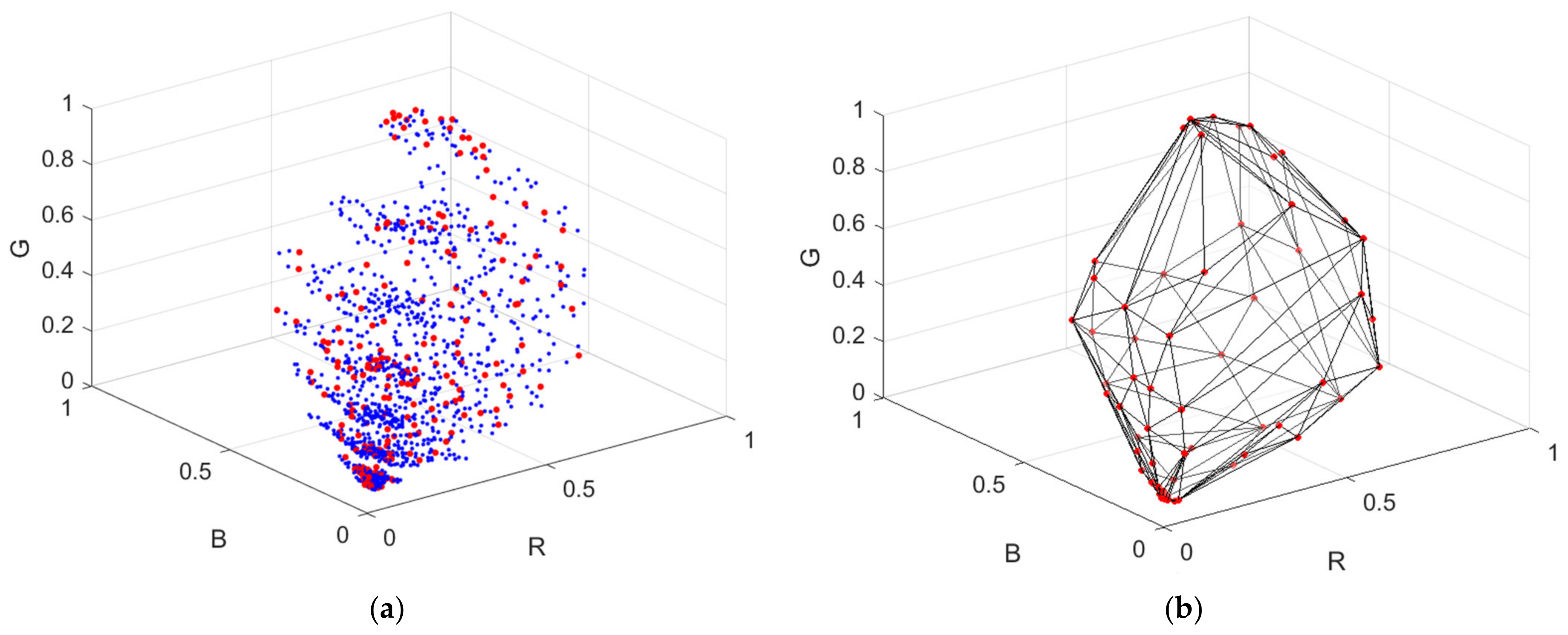
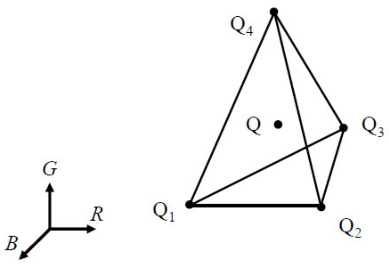
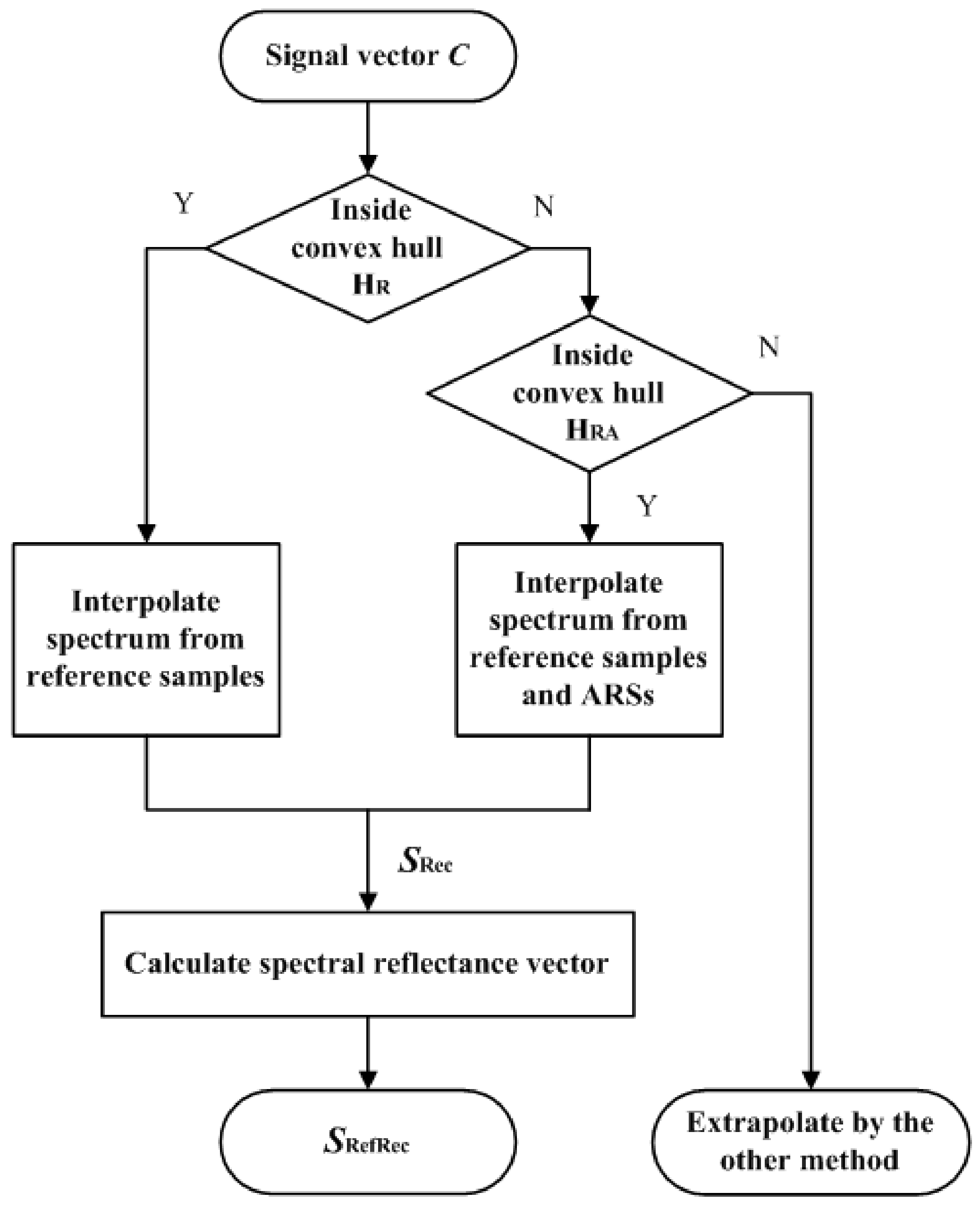
Table 4 shows the assessment metric statistics for the test samples using the LUT method, where the Nikon D5100 and CMF cameras were used. As can be seen from
Table 4, out of the 1066 test samples, about 860 samples were inside samples that can be interpolated. The table also shows the extrapolation results for about 200 outside samples, which are discussed in the next subsection. The assessment metric statistics for the inside samples using the two cameras were about the same except for the color difference Δ
E00. If the spectral sensitivities of a camera are different from the CMFs, the color difference Δ
E00 will be a non-zero value from Equations (1a) and (2). While not zero, most of the inside samples using the Nikon D5100 showed little color difference.
The spectrum reconstructions of the test samples using the PCA and wPCA methods are considered for comparison. In the wPCA method, the
i-th training sample was multiplied by a weighting factor 1/(Δ
Ei +
s), where Δ
Ei is the color difference between the test sample and the
i-th training sample in CIELAB;
s is a small-valued constant to avoid division by zero [
8]. Weighted training samples were used to derive basis spectra. A camera device model was used to convert RGB signal values into tristimulus values for calculating Δ
Ei. A third-order root polynomial regression model (RPRM) was employed and trained using the reference samples [
30]. The accuracy of the RPRM was slightly higher than that of the polynomial regression model in this case.
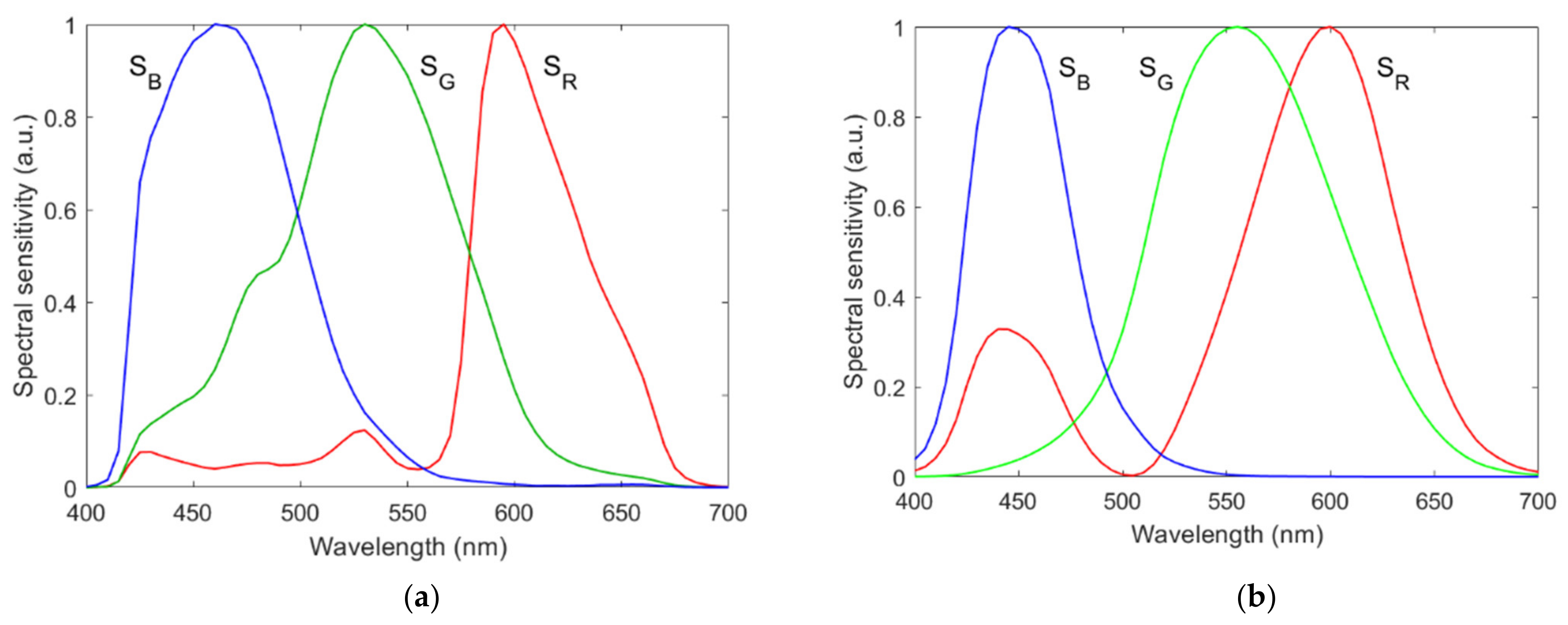
The PCA and wPCA methods were used to reconstruct all test samples using the spectral sensitivities of the Nikon D5100 in
Figure 1a.
Table 5 shows the assessment metric statistics for the test samples using the PCA and wPCA methods, where the inside samples and outside samples were the same as those using the LUT method. The spectrum reconstruction error using the wPCA method was apparently smaller than that using the PCA method, as expected. Comparing
Table 4 with
Table 5, we can see that the LUT method outperformed the wPCA method except for
GFC.
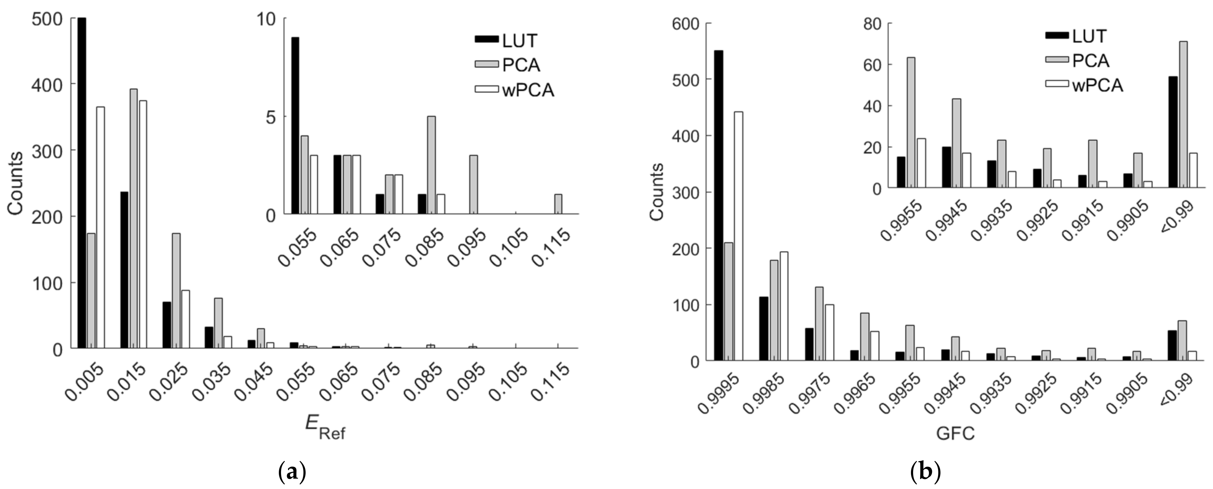
Figure 11a,b show the
ERef and
GFC histograms for the 864 inside samples, respectively, where the cases using the LUT, PCA and wPCA methods are shown.
The computation time required for the LUT method is at least two orders of magnitude faster than that required for reconstruction methods using basis spectra that emphasize the relationship between the test and training samples [
13]. In this work, the ratio of the computation time required to use the LUT method and wPCA method was 1:80.2, where samples were reconstructed from their signal vector
C to the spectral reflectance vector
SRefRec using MATLAB on the Windows 10 platform.
5.2. Extrapolation Using the LUT Method Utilizing Optimized ARSs
The color filters optimized as in
Section 4.2 were used to create the ARSs in this subsection. The edge wavelengths of the optimized color filters for the Nikon D5100 and CMF cameras are shown in
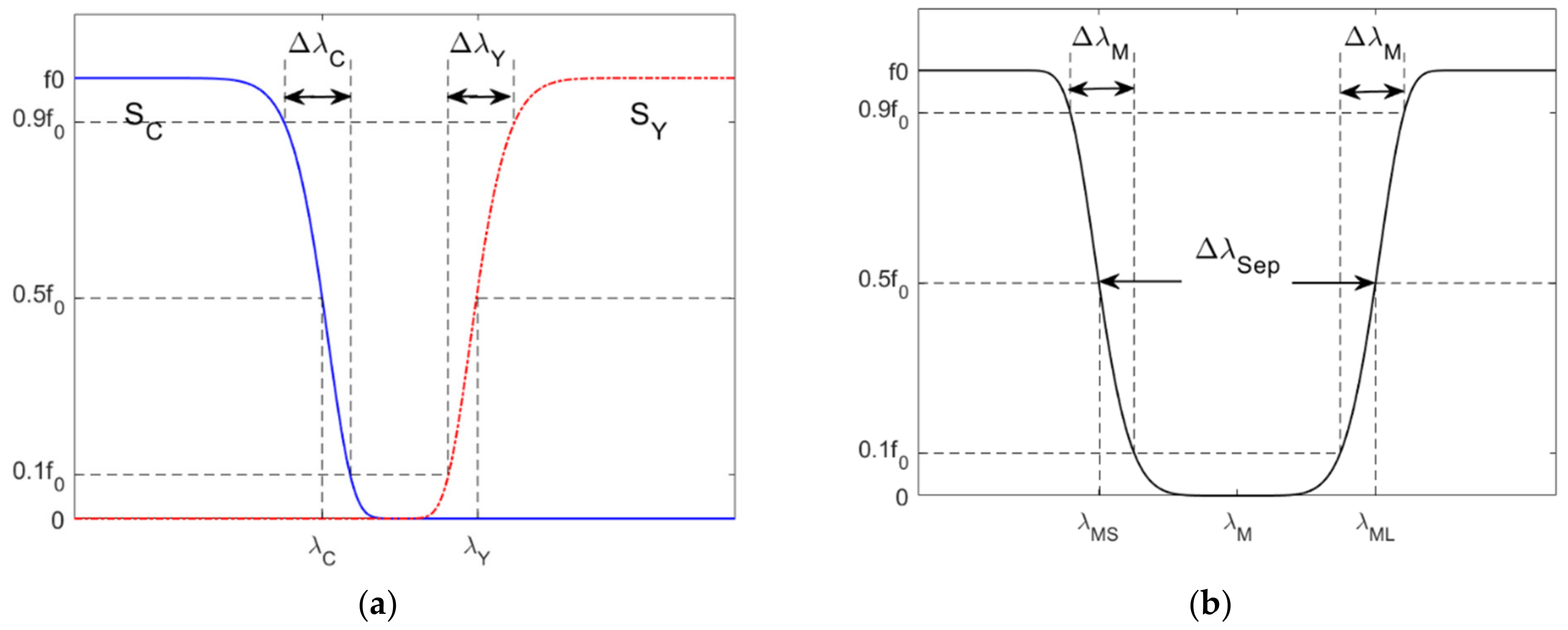
Table 3. The filter spectral transmittance for the Nikon D5100 and CMF cameras is shown in
Figure 7a,b, respectively. From
Table 4, there were 202 and 203 outside samples for the Nikon D5100 and CMF cameras, respectively. The assessment metric statistics for the outside samples are shown in
Table 4. As expected, the mean assessment metrics for the outside samples were worse than those for the inside samples. The assessment metric statistics for the two cameras were about the same except for the color difference Δ
E00. The assessment metric statistics for all samples are also shown in
Table 4.
For the Nikon D5100, there were 98, 79, 22 and 3 outside samples that referenced 1, 2, 3 and 4 ARSs, respectively.
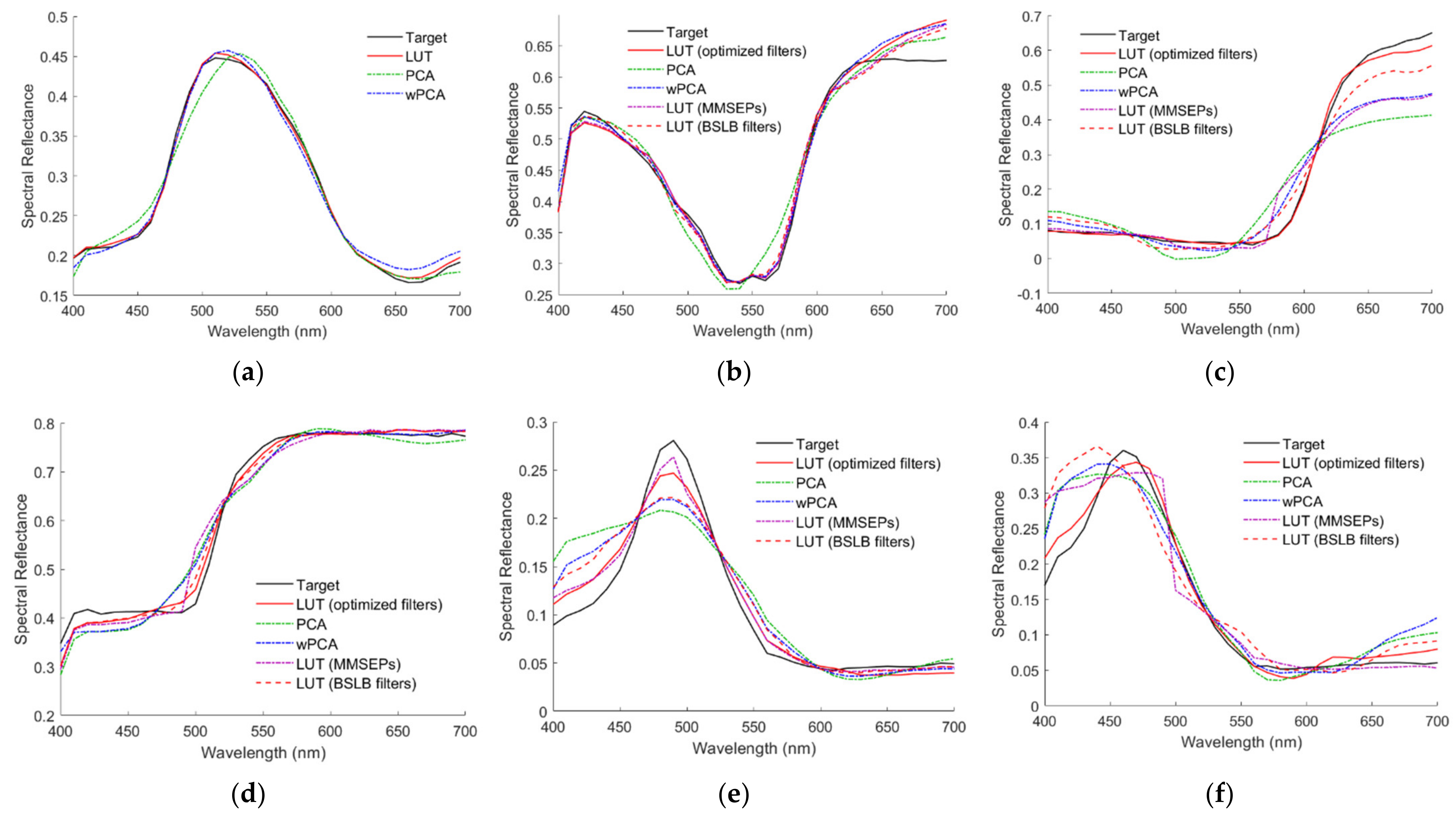
Figure 12a–f show the reconstructed spectra
SRec using the LUT method for the 2.5G 7/6, 10P 7/8, 2.5R 4/12, 2.5Y 9/4, 10BG 4/8 and 5PB 4/12 color chips, respectively, where their target spectrum
SReflection and neighboring reference spectra are also shown. The case in
Figure 12a is an interpolation example for comparison. The cases in
Figure 12b–f are extrapolation examples. For the cases in
Figure 12b–f, the numbers of referenced ARSs are 1, 2, 2, 3 and 4, respectively. The ARS neighborhoods are indicated in the figures. Neighborhood 3 is the black ARS for the case in
Figure 12e. The spectrum was well recovered for the case in
Figure 12f, although four ARSs were referenced. The reconstructed spectral reflectance
SRefRec for the cases in
Figure 12a–f is shown in
Figure 13a–f, respectively. RMS errors
ERef = 0.004, 0.0223, 0.014, 0.0165, 0.0159 and 0.0149 for the cases in
Figure 13a–f, respectively.
5.4. Effect of Filter Edge Wavelengths
The spectral sensitivities of a camera can be measured or estimated as described in
Section 1. If the measurements or estimates are accurate, the color filters can be optimized using the same method as in
Section 4.2. On the other hand, estimates of sensitivity spectral shapes may not be very accurate, but estimates of channel wavelengths may be accurate enough for color filter design. It is found that the specifications of optimized color filters are related to the channel wavelengths. For the Nikon D5100, from
Table 2 and
Table 3, the optimized edge wavelengths
λCopt,
λYopt,
λMSopt and
λMLopt are about
λCamR +Δ
λCamR/4, (
λCamC +
λCamG)/2,
λCamC and
λCamR, respectively, where
λCamC is an average wavelength and
These approximate relationships are roughly valid for the CMF camera. Since the channel wavelength is the average wavelength of the spectral sensitivity, the specifications of appropriate color filters could be estimated from less accurate estimates of the spectral sensitivities.
In this subsection, the use of color filters that are not optimized is studied. Deviations of filter specifications from their optimized values are expressed as δ
λC =
λC −
λCopt, δ
λY =
λY −
λYopt, δ
λMS =
λMS −
λMSopt and δ
λML =
λML −
λMLopt. It is found that the appropriate range of edge wavelengths can be roughly estimated as
where
λCamY is an average wavelength and
For the Nikon D5100,
λCamC = 498.7 nm and
λCamY = 567 nm. The empirical estimates shown in Equation (12a–d) are based on the comparison of
Figure 7a,b with
Figure 1a,b, respectively, and the tolerance analysis shown below.
The deviation of the edge wavelength from the optimized value results in a change in the convex hull HRA. Since λCopt > λCamR, increasing positive δλC will result in an increase in the R signal with little change in the B and G signals, which will cause the ratios B/R and G/R to decrease. The decrease in the signal saturation results in a smaller convex hull HRA in the cyan region, and some outside samples may not be extrapolated. Therefore, the upper bound in Equation (12a) is set to the optimized edge wavelength of the cyan filter. The upper bounds in Equation (12b–d) are changed for similar reasons. Since λCamC < λYopt < λCamG, increasing positive δλY will result in a greater reduction in the G signal, which will cause the ratio G/B to decrease. Since λMSopt ≈ λCamC and λMLopt ≈ λCamR, increasing positive δλMS and δλML will result in a greater increase in the G signal and a greater reduction in the R signal, respectively, which will cause the ratios B/G and R/G to decrease.
Figure 15a–i show the mean RMS error
ERef of outside samples versus δ
λMS and δ
λML, where the values of δ
λC and δ
λY are shown in the figures. The camera is the Nikon D5100. In the figures, δ
λC = −51.9 nm and −15.5 nm correspond to
λC =
λCamY and
λCamR, respectively; δ
λY = −12.1 nm corresponds to
λY =
λCamC. The white symbols “+” and “x” are the origin (δ
λMS = δ
λML = 0 nm) and the point of the minimum mean
ERef in each figure, respectively. The values of the mean
ERef at the origin and at the point of the minimum mean
ERef are shown in
Table 8 and
Table 9, respectively, for the cases in
Figure 15a–i. In the two tables, the corresponding filter edge wavelength deviations and the ratio
RGF99 are also shown.
At the origin in
Figure 15a–i, all outside samples can be extrapolated. Away from the origin, the red dotted line represents the boundary where at least one outside sample cannot be extrapolated. Beyond the boundary, the mean
ERef of outside samples that can be extrapolated is shown. The white dotted line in the figure represents the contour of the mean
ERef = 0.0213, which is the value obtained using the wPCA method. Using color filters that meet the specifications within both the red and white dotted lines, all outside samples can be extrapolated while keeping the mean
ERef < 0.0213. For the cases with δ
λC = 0 in
Figure 15c,f,i, the area enclosed by the red and white dotted lines is small because some cyan outside samples cannot be extrapolated. They can be extrapolated by using a blue-shift cyan filter, i.e., δ
λC < 0, but will increase the extrapolation error. When δ
λC = −9.0 nm, the red dotted line is about the same as in the cases of δ
λC = −15.5 nm in
Figure 15b,e,h. Therefore, if a larger edge wavelength tolerance is required, a blue-shift cyan filter is preferred. For such a requirement, the upper bound
λCopt in Equation (12a) can be replaced by
λCamR.
The point of (δ
λML, δ
λMS) = (−41.1 nm, −33 nm) in
Figure 15g is the lower bound case in Equation (12a–d), where
λC =
λCamY,
λY =
λCamC,
λMS =
λCamB and
λML =
λCamY. Since all filter edge wavelengths are blue-shifted, this case is called the blue-shift lower bound (BSLB) case. In contrast, the upper bound case in Equation (12a–d) is the optimized case at the origin in
Figure 15c. The assessment metric statistics of the BSLB case are shown in
Table 6, where the mean
ERef = 0.019 and
RGF99 = 0.8416. As can be seen from
Table 6, the assessment metric statistics of the BSLB case were worse than those of the optimized case, but better than those of the wPCA and NTCC methods.
Figure 13b–f also show the reconstructed spectral reflectance of the BSLB case, where the RMS errors
ERef = 0.0187, 0.0469, 0.0203, 0.0274 and 0.0482, respectively.
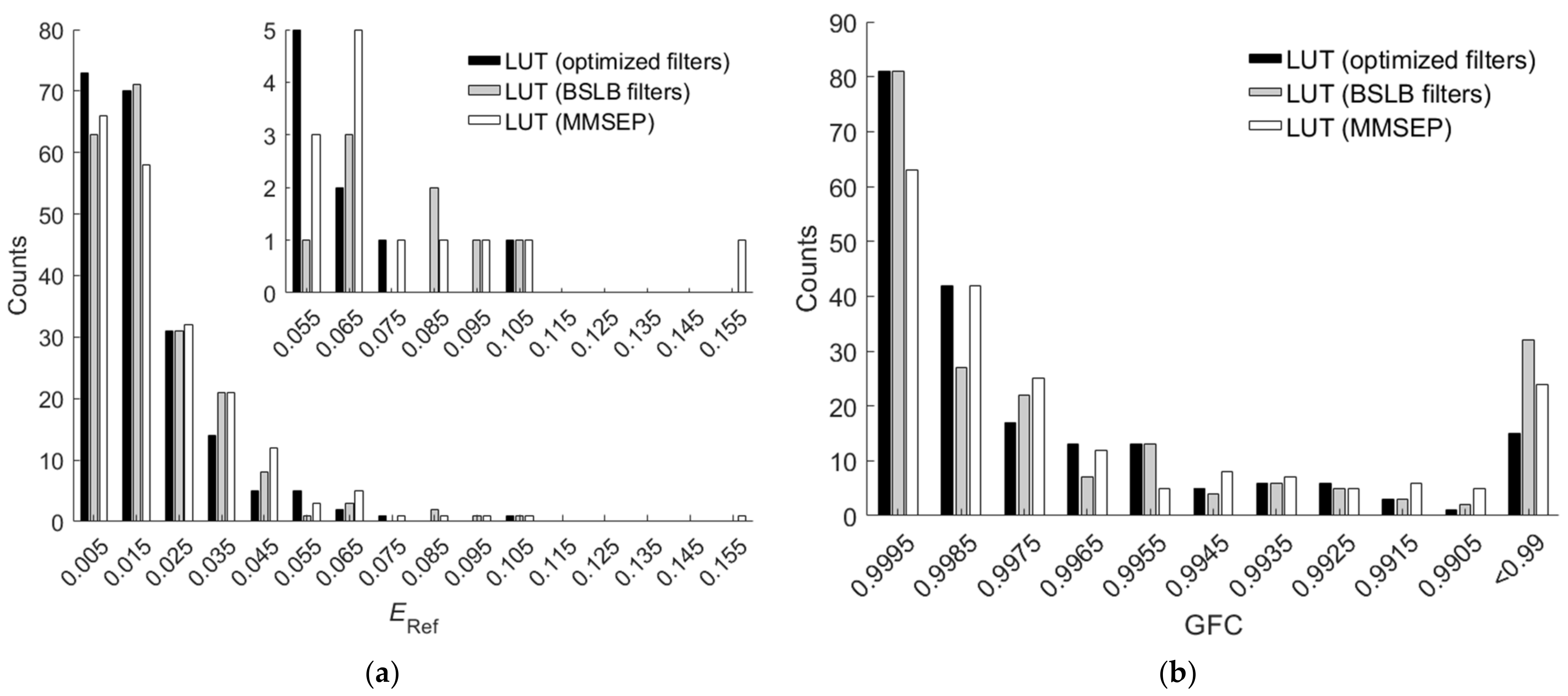
Figure 16a,b show the
ERef and
GFC histograms, respectively, for the 202 outside samples of the BSLB case. Also shown are the results of the cases using the LUT method utilizing optimized ARSs and the LUT method utilizing MMSEP samples for comparison. As can be seen from the two figures and
Table 6, for the RMS error
ERef, the unoptimized BSLB case was slightly better than the case including MMSEP samples, but for the goodness-of-fit coefficient
GFC, the case including MMSEP samples was slightly better. The extrapolation performance of the two cases is comparable. Note that it is easy to design better color filters than the BSLB case for extrapolation.
