3.1. Time Series Building and Data Clustering
Training data, for each of the 10 patients, was comprised of 360 meals and 119 night events, of varying duration. The number of hypoglycemia treatment events was patient-dependent, attending to the settings of the open loop therapy provided in the simulator, with a median value of 18 events and 25–75% percentiles of 13 and 36 events, respectively. Mean CGM glucose ranged from 122 mg/dL (patient 10) to 169 mg/dL (patient 7).
Application of the PDSFCM clustering algorithm, in combination with the FS cluster validity index for the determination of the number of clusters, resulted in a varying number of clusters depending on the variability exhibited by the patient, as shown in
Table 1.
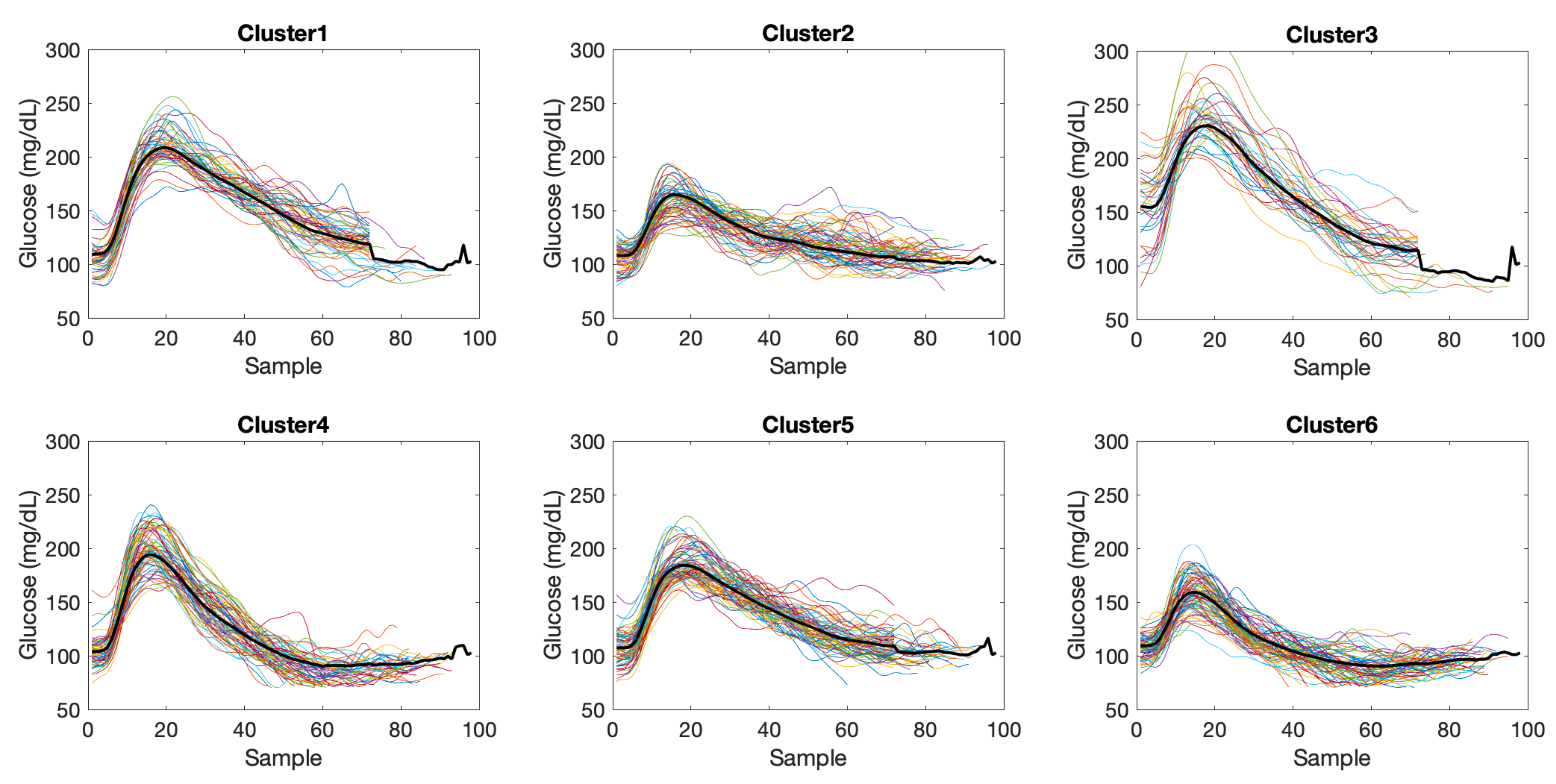
As an illustration,
Figure 5 shows the clustering results for patient 6 and data in the meals partition
. The number of elements per cluster were 50, 61, 36, 63, 70 and 71 for clusters 1 to 6, respectively. Regularized length of the time subseries was 98. Considering the whole cohort, regularized lengths ranged from 98 to 106 samples for
, from 60 to 65 samples for
, and from 36 to 76 samples for
.
After clustering, time subseries were assigned to the cluster with maximum membership. Then, a seasonal time series per cluster was created by concatenating all time subseries assigned to the given cluster representing similar glycemic excursions, preceded by pre-sampling data. A length of five samples was considered for pre-sampling data (
), given that orders lower than 5 were obtained for the AR and MA processes in previous studies. Thus, a seasonality period of
was enforced, with
L the regularized length for that patient and data partition. The resulting seasonalities are presented in
Table 2.
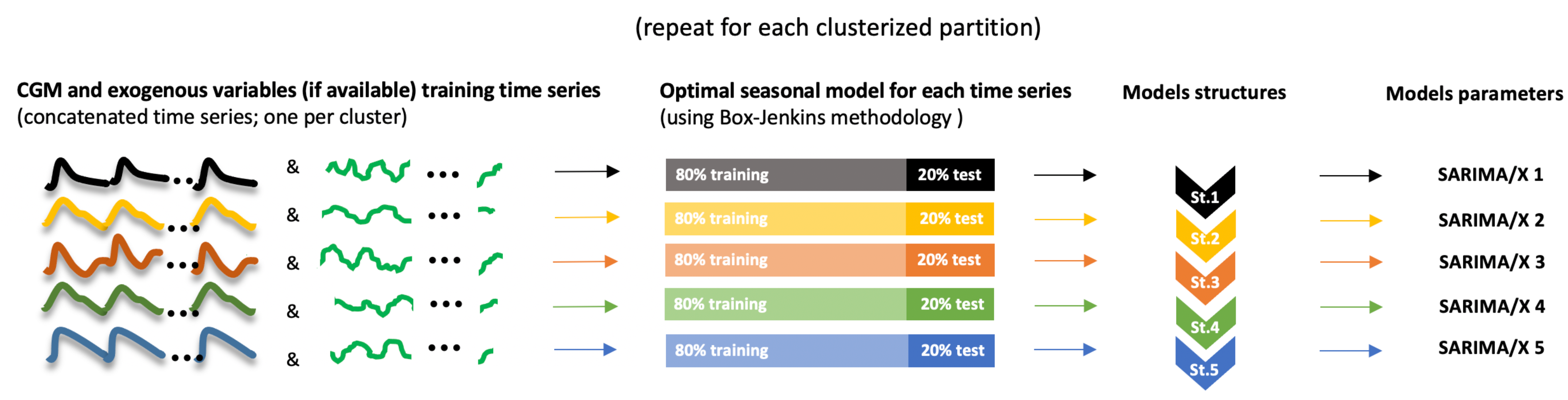
3.2. Local Models Identification
A model for each cluster was identified using the Box-Jenkins methodology. As stated in
Section 2.7, the first 80% of the data in a cluster were used for model identification, and the rest 20% for model evaluation. During the identification, residuals at time instants with missing values or belonging to pre-sampling periods in the concatenated time series were neglected (weighted 0 in the cost index). SARIMA model structure and parameters were identified for each cluster.
Table 3 shows, as an example, the resulting SARIMA model structure
for each cluster for patient 6. The orders for the AR component (
p) ranges from 1 to 4, and for the MA component (
q) from 0 to 4. With regards to seasonal part, SAR component order (
P) ranges from 1 to 2, and SMA order (
Q) from 0 to 2. Need for time series differentiation (
or
) only appeared in hypoglycemia treatment cases, where glucose may follow an increasing trend. Similar results were obtained for the rest of patients.
Accuracy metrics of the trained local models is shown in
Table 4, aggregating data for all patients and local models in a partition, as well as overall metrics. For all prediction horizons, the lowest metrics were obtained for the night partition
due to the lower variability during nights as compared to meals. Local models for
had a poorer performance due to the significantly lower number of events for training and validation, compared to
and
. Comparing
versus
, the latter reported higher values, since residuals of the last predicted value in each prediction is expected to be higher than when the whole predicted trajectory is considered. However, the higher the prediction horizon, the lower this difference was. This may be due to the implicit exclusion of residuals in
in the computation of
, where
is the event initial time. When
is long enough, an important part of a postprandial response may be neglected, which may provoke a loss of monotonicity of the
metrics with respect to the prediction horizon. Overall performance was good, with a maximum average
of 11.46 mg/dL (
of 6.79%), corresponding to a PH of 240 min. Maximum average
was 13.69 mg/dL (for a PH of 180 min), and maximum average
of 8.86% (for a PH of 240 min). During the night predictions, these metrics were reduced approximately by 40%.
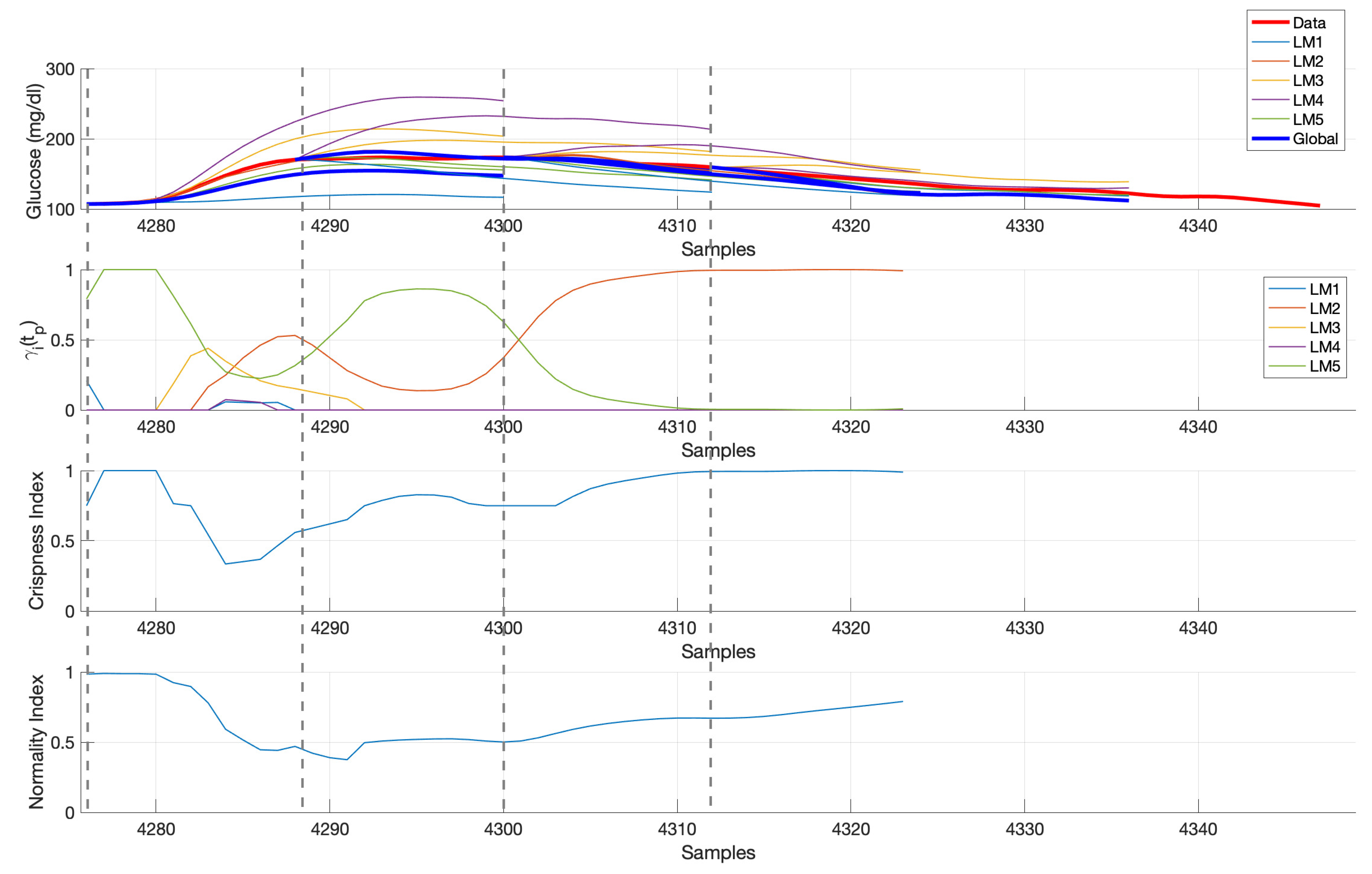
3.3. Online Forecasting Validation
Figure 6 shows an illustration of the real-time computation of glucose predictions considering 5 local models for a sample validation time subseries in
. Four 120-min ahead predictions are shown, separated one hour each, at the samples indicated by the vertical dashed lines starting at mealtime. Upper panel shows CGM data, local models predictions and global glucose prediction obtained from the weighted sum of local predictions, with time-varying weights are shown in the
panel. Early postprandial response is more variable and, thus, more local models contribute to the glucose prediction computation, compared to late postprandial phase, where LM2 seems to fully describe the response in this case. This is also described by the crispness index, with lower values at time instants where a higher number of local models contribute to the predicted trajectory. The normality index describes to what extent past short-time CGM data at each prediction time
is represented by the same segment of data from cluster prototypes, and “interpolation” instead of “extrapolation” is being performed. In this case, a drop of the index is observed during the glucose increase until peak value. A too low value would indicate an abnormal behavior, which threshold need to be tuned (see
Section 3.4).
Table 5 present validation results of the glucose predictor in real-time operation for the 2-month independent validation dataset 1 (“normal”) described in
Section 2.1. Metrics are expected to deteriorate as compared to the local models performance due to the local predictions integration process, as it is observed in the data presented. For this dataset, overall average
ranged from 3.51 mg/dL to 23.90 mg/dL for prediction horizons 15, 30, 60, 120, 180 and 240 min (
from 2.35% to 15.19%). Overall average
ranged from 6.52 mg/dL to 28.96 mg/dL (
from 4.04% to 20.00%).
Table 6 presents validation results for the two month independent validation dataset 2 (“abnormal”) described in
Section 2.1. Inclusion of abnormal events slightly increased error in 1–2% as comparison of
and
in
Table 5 and
Table 6 reveal. This was expected since missed boluses and exercise were not present in the training. The impact was higher up to a prediction horizon of 120 min, which may be related to the duration of the abnormal event effect on glycemia (postprandial and post-exercise periods). The number of predictions column indicates that abnormal events increased the number of hypoglycemic episodes (due to exercise), inducing different partitioning of data and participation of the glucose predictors for
,
, and
. For the abnormal dataset, overall average
ranged from 4.04 mg/dL to 25.36 mg/dL for the PHs considered (
from 2.65% to 15.06%). Overall average
ranged from 7.33 mg/dL to 32.83 mg/dL (
from 4.66% to 19.82%).
Other authors have conducted in silico studies for the performance analysis of a variety of prediction methods, although comparison is not straightforward due to the difference in the simulators used, scenarios considered, and different input requirements by the glucose prediction technique. In this sense, the lower the inputs needed to perform a prediction the better, especially when such inputs require patient intervention such as the amount of carbs intake, for instance. These results are summarized in
Table 7.
In [
24], 8-day glucose and insulin data is used from a virtual cohort of 30 patients from the educational version of the UVA/Padova simulator, comprising 10 adults, 10 adolescents and 10 children. Variability in meal time and quantity was considered. Three models are compared: AR, ARX considering insulin as input, and ANN (artificial neural network), with prediction horizons of 30 min and 45 min. For the adult population,
values of 14.0 mg/dL, 13.3 mg/dL and 2.8 mg/dL are reported for AR, ARX and ANN with prediction horizon 30 min, respectively. These figures increase to 23.2 mg/dL, 22.8 mg/dL, and 4.0 mg/dL for a prediction horizon of 45 min. ANN outperformed AR and ARX models. Compared to results in
Table 5, AR and ARX are outperformed by the methodology here presented, with a
of 11.32 mg/dL for a prediction horizon of 30 min. This is as well the case for results in
Table 6 including abnormal data, where an
of 13.18 mg/dL was achieved. Metrics obtained for AR and ARX for 45 min are comparable to the metrics reported in
Table 5 for a prediction horizon of 120 min (
mg/dL), and in
Table 6 for 60 min (
mg/dL), respectively. However, this is not the case for ANN, with extremely low
values reported in [
24]. This may be due to the nature of the in silico study, since the simulator used in [
24] does not include the extra features of intra-patient variability reported in
Section 2.1, besides the length of the data (8 day vs. 2 months), which might have produced overfitting in the ANN case. As well, the ANN used insulin data as external input which may limit applicability to insulin pump users, while in our case, only glucose and mealtime is used for glucose prediction. This latter can be extracted from the pump or smart pen information, or even estimated using meal detection algorithms in standard insulin pen users.
In [
25], a neural network incorporating meal information in parallel with a linear predictor (NN-LPA) is evaluated in silico with 11-day data from 20 subjects of the UVA/Padova simulator. As in the previous case, variability in meal time and quantity was considered. The method is compared with the neural network presented in [
30] (NNPG) and an AR(1) model. For a prediction horizon of 30 min,
values of 9.4 mg/dL, 10.7 mg/dL, and 17.5 mg/dL are reported for NN-LPA, NNPG and AR(1), respectively. Of note, NN-LPA requires a physiological meal model since the glucose rate of appearance at
is one of the inputs of the neural network. In [
26], a latent variable-based model (LVX) is evaluated from 7-day data from 10 virtual subjects of the UVA/Padova simulator. The model used meal intake and insulin information as exogenous variables. An average
of 8.6 mg/dL and 14.0 mg/dL was reported for 30-min and 60-min prediction horizons, respectively, as compared to our results in
Table 5 with an
of 11.32 mg/dL and 17.85 mg/dL, respectively, and
Table 6, with 13.18 mg/dL and 21.00 mg/dL, respectively. A slight increase of
of only approximately 3–4 mg/dL (5–7 mg/dL with abnormal data) is observed in our results, despite the far more challenging intra-patient variability in our work and less input information required, as stated above.
More recent in silico studies, in this case using the same extended UVA/Padova simulator as in this work, have been reported. In [
27], a physiological model (PM) in combination with CGM signal deconvolution is presented for long-term glucose prediction. The model requires as inputs carbohydrate intake and insulin delivery, as opposed to our case. Two-week data for 10 in silico subjects is used for model training and evaluation.
values of 10.90 mg/dL, 24.44 mg/dL, 33.50 mg/dL, and 37.63 mg/dL are reported for prediction horizons of 30, 60, 90 and 120 min. These values outperformed ARX and LVX models in head-to-head comparisons. In [
28], convolutional recurrent neural networks (CRNN) are evaluated with 1-year data from 10 in silico subjects. Models are trained with 50% of the data and evaluated with the rest 50%. Glucose, meal and insulin information are required as inputs.
values of 9.38 mg/dL and 18.87 mg/dL for 30-min and 60-min prediction horizons are reported. Above metrics are outperformed in general by results presented in
Table 5 and
Table 6, being especially relevant longer prediction horizons. Finally, in [
29] dilated recurrent neural networks (DRNN) are tested with the same 1-year in silico study. A prediction horizon of 30 min is considered, with a reported
of 7.8 mg/dL, which is better than our result for the same prediction horizon even in the absence of abnormal data (11.32 mg/dL). However, DRNN required information on insulin, meal intake and time of the day, as opposed to this work.
Summing up, with the limitation of a non-head-to-head comparison and variety of simulation studies in the literature, metrics obtained outperformed other methods, or were very close to the reported performance. This was so even when imperfect training was considered introducing abnormal data in the validation dataset, while having the clear advantage of the minimal input information required (CGM and mealtime). This one can ultimately be automatically extracted without patient intervention making the glucose predictor suitable for insulin pump and MDI users.
From the point of view of the real-world application of the methodology, it is worth remarking that, in a similar way to a neural network, the training phase is the one more computationally demanding. In this work the computing cluster Rigel from Universitat Politècnica de València was used, in particular the Dell Power Edge R640 nodes with 2 processors Intel Xeon Gold 6154 with 18 cores, 3 Ghz and 25 Mb cache memory. The clustering phase for the 10 patients, which included 10 clustering problems per patient with increasing number of clusters for later selecting the optimal number of them, using 22 cores and 3 Gb memory per core, was computed in 22 min. The training of the local models, using 30 cores and 3 Gb memory per core, was performed in about 6.5 h. Validation of local models, using the same resources, lasted 53 min. This gives rise to a total of 8 h of computing time approximately for training. Once trained, the real-time evaluation of a glucose prediction is straightforward, requiring the evaluation of equations in
Section 2.5 for the glucose prediction (evaluation of
n SARIMA models,
n fuzzy memberships, and a weighted sum of time series, where
n is the number of clusters), and
Section 2.6 for crispness and normality indices.
3.4. Normality Index
The Normality Index defined in Equation (
23) is intended to provide information on abnormal glucose behaviors according to available historical data. Thus, it is expected that low normality values at time
,
, are related to higher prediction errors for glucose trajectories computed at that same time
. The Normality Index relies on the comparison of CGM values in the recent past (20 min in this work) with cluster prototypes in that same time window. It is expected that this relationship with the prediction error is stronger for short or medium prediction horizons, for which abnormal behavior is still present. A PH of 60 min was considered in the following analysis. All predictions
,
, carried out during the validation of the glucose predictor for dataset 2 (“abnormal”), amounting to a total of 138,888 predicted trajectories, were grouped into two groups, for
and
, with the threshold
varying from 0.1 to 0.9 in steps of 0.1. Then, the difference of the median prediction error at
(absolute value of the residual) among groups was analyzed. Remark that these residuals are the ones considered in the computation of
for a given validation time subseries.
Figure 7 shows these results. All differences were found statistically significant using the Wilcoxon Rank Sum test (
). This test was selected since data was non-normal and non-paired.
Clinically meaningful differences were obtained for the lowest thresholds, amounting to 19.14 mg/dL for
, and 10.29 mg/dL for
. As an illustration,
Figure 8 shows the relationship for
, which reveals an increased presence of higher prediction errors when
(median [25th–75th percentiles]: 21.05 [9.79, 38.52] vs. 10.75 [4.88, 20.49] mg/dL).
Finally,
Figure 9 illustrates an example of the relationship between NI and abnormal events in the simulated scenario. Postprandial response after a missed bolus (blue shaded area) is clearly detected as an abnormal CGM response. Consider that a minimum delay of 20 min will happen since that is the window considered in the computation of NI. After an initial glucose rise that could be similar to other meals, the value of NI is below the threshold consecutively at each sample during the postprandial period until glucose returns to normoglycemia. Regarding the exercise, including 3-h post-exercise period with altered insulin sensitivity (green area), abnormality is found in the hypoglycemia recovery, due to the increased need of carbohydrates as compared to a non-exercise related hypoglycemia in the training data, as well as the initial response of the meal following exercise. Other segments of CGM data might be also considered abnormal without relation to missed boluses or exercise, such as the one around sample
. In this case, a meal close to a hypoglycemia recovery happened.
The information provided by the Normality Index can be useful in real-time operation, raising for instance warnings when sufficiently long abnormal periods are detected (as in the case of missed boluses), due to expected decrease of accuracy of predictions. Additionally, remark that its computation is independent of predictions since it relies only on the clustering training phase (no local models are implied). This means that its use in an offline context can also be devised, as a tool for the analysis of CGM data highlighting areas of abnormal response that may deserve special attention by the clinician.


