Abstract
How to operate an unmanned aerial vehicle (UAV) safely and efficiently in an interactive environment is challenging. A large amount of research has been devoted to improve the intelligence of a UAV while performing a mission, where finding an optimal maneuver decision-making policy of the UAV has become one of the key issues when we attempt to enable the UAV autonomy. In this paper, we propose a maneuver decision-making algorithm based on deep reinforcement learning, which generates efficient maneuvers for a UAV agent to execute the airdrop mission autonomously in an interactive environment. Particularly, the training set of the learning algorithm by the Prioritized Experience Replay is constructed, that can accelerate the convergence speed of decision network training in the algorithm. It is shown that a desirable and effective maneuver decision-making policy can be found by extensive experimental results.
1. Introduction
With the development of the control and electronic techniques in recent years, the performance of unmanned aerial vehicle (UAV) has been improved rapidly in all aspects. The UAV has been applied to assisting, replacing people to complete difficult missions due to high mobility, great flying height, and low cost [1]. Thus, it is necessary to improve the autonomy of UAV while performing some special airdrop tasks without risking human lives, such as delivery of relief supplies [2], extinguishing by UAV, and so on. Consequently, how to improve the autonomous flight capability of UAV becomes the research focus of researchers in various countries [3].
At present, the airdrop tasks are typically implemented incorporating with path panning [4], which is a method for searching an optimal path from start point to end point while avoiding obstacles in the environment. Conventional path planning algorithms for UAVs include Visibility Graph [5,6]; randomly sampling search algorithms, like Rapidly-exploring Random Tree [7], Probabilistic Roadmap [8]; heuristic algorithms, such as A-Star [9], Sparse A-Star (SAS) [10], and D* [11]; and genetic algorithms [12]. Then, a UAV can fly to target point by following the planned route, where various trajectory tracking algorithms are proposed [13,14]. However, this kind of schemes have some disadvantages. For example, an optimal route relies on a priori knowledge about the environment, in which the data of terrain and obstacles is usually difficult to obtain, limiting our capability of environment modelling. Moreover, when the environment becomes dynamic, involving moving obstacles, these schemes are not flexible enough to alter their control strategies immediately. A replan of paths have to be scheduled to adapt to the changes in the environment. Therefore, it is desired to design an end-to-end algorithm that can manipulate a UAV to flight autonomously in a dynamic environment without path planning and trajectory tracking.
A promising direction is inspired by the AlphaGo developed by Google based on deep reinforcement learning, which can play Atari games using a kind of end-to-end decision-making algorithm, called Deep Q Network (DQN) [15]. The performance of this algorithm reached human level after an extensive training, which shows the potential of the reinforcement learning-based methods combined with deep learning in solving practical problems. Meanwhile, in order to solve the dimension explosion caused by the continuity of action space, the Deep Deterministic Policy Gradient (DDPG) was proposed in Reference [16], and the experience replay is used in these Deep Reinforcement Learning (DRL)-based algorithms and allow agents to remember and learn from historical data. The DDPG overcomes the dimension explosion issue caused by continuous action space and state space. However, it forms training set by taking samples from data memory with the Uniform Experience Replay (UER), which does not fully exploit the diversity of historical data. Moreover, the UER usually has a low convergence rate of neural network and even divergence in training neural networks. Therefore, the Prioritized Experience Replay (PER) was proposed to improve the efficiency of learning from experiences [17]. In this paper, we construct a new priority of each experience based on Double Q-Learning [18], which could overcome convergence fluctuation caused by over estimate compared with Reference [19].
In the present work, we aim to tackle the challenges mentioned above and focus on the UAV maneuver decision-making for airdrop task. The main works presented in this paper are summarized as follows:
- The UAV Maneuver Decision-Making Model for airdrop tasks is built based on Markov Decision Processes (MDPs). Particularly, we design the flight state space, the flight action space, and the reward functions. Among the components of model, we devote our air-to-ground drop theory to designing and constructing the UAV maneuver decision-making model for airdrop tasks.
- We propose the Maneuver Decision-Making Algorithm for autonomous airdrop based on DDPG with PER sampling method (PER-DDPG) to train a UAV for generating efficient maneuver under target point constraint refined from the model we designed in an interactive environment. Specially, we design the decision-making function by deep neural network and construct the training set sampling method based on PER.
- Simulation results show that the algorithm we proposed could improve the autonomy of a UAV during the airdrop task and the PER is able to accelerate the efficiency of learning from experiences. Moreover, we find that the winning rate of the PER-based algorithm exceeds the UER-based algorithm 2–4%.
This paper is organized as follows: Section 2 describes the background knowledge of all the methods used to design UAV maneuver decision-making model and algorithm. Section 3 presents the details of experimentations we designed, comparison of learning rate and winning rate under UER and PER sampling methods separately. Section 4 shows the conclusion of our work and looks forward to the future of our research.
2. Methodology
The UAV has been used to help people finish some dangerous and repetitive missions, such as crop protection, wildlife surveillance, traffic monitoring, electric power inspection, search, and rescue operations. A need for more advanced and simple UAV autonomous flight solution has emerged. As mentioned above, traditional solution of real time obstacle avoidance for manipulators and UAVs is that algorithm plans an optimal path and then UAV follows path by trajectory tracking method. In this paper, we redefined the process of UAV autonomous flight and constructed the UAV Maneuver Decision-Making Model for Airdrop Task based on MDPs [20]. On the other hand, we proposed a novel UAV Maneuver Decision-Making algorithm based on Deep Reinforcement Learning [21].
As shown in Figure 1, we construct the UAV Maneuver Decision-Making Model for Airdrop Task Based on MDPs firstly. Among this model, we design the flight action space, the flight state space and flight assessment function that are used to demonstrate the characteristics of UAV autonomous flight during airdrop. Moreover, we design and realize the UAV Maneuver Decision-Making Algorithm, including the UAV maneuver decision-making network, prioritized experience replay used to sample training data from historical experiences, and network optimizer applied to train networks.
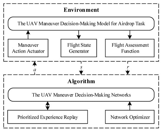
Figure 1.
The structure of unmanned aerial vehicle (UAV) Maneuver Decision-Making Algorithm.
2.1. The UAV Maneuver Decision-Making Model for Airdrop Task Based on Mdps
2.1.1. Markov Decision Processes
During the process of performing airdrop task, UAV maneuver decision-making could be regarded as a sequential decision process. Moreover, while selecting optimal action for UAV, the controller usually considers current information from environment. Thus, we can think that this decision process is Markovian and could use MDPs to model the UAV maneuver decision-making model for airdrop task.
MDPs can be described by a quintuple
where T represents the decision time, S represents the system state space, represents the system action space, and the transition probability represents the probability distribution of the system at the next moment when the system used the action in the state . The reward function represents the benefit that the decision-maker gets when the action is taken in the state . Based on the MDPs, we can define a complete mathematical description of the UAV Airdrop Task.
As shown in Figure 2, MDPs can be summarized as follows: the initial state of the system is that the decision-maker chooses action and executes it, system moves to next state according to a certain transition probability , and so on. In this process, the decision-maker earned rewards sequence . Among this process, the decision-maker is stimulated by external rewards, and rewards are maximized by constantly updating policy. The action adopted by decision-maker is , where is effective policy, and the utility function (at state , the expected reward obtained by adopting the policy ) is . When current policy is the optimal policy, Equation (2) should be satisfied.
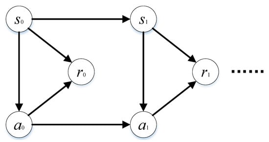
Figure 2.
The structure of finite Markov Decision Processes (MDPs).
Based on the characteristics of UAV maneuver decision-making for airdrop, we use infinite stage discount model as utility function, as shown in Equation (3).
In the equation above, is the future reward discount factor. represents mathematical expectation; thus, Equation (3) indicates that the expected objective of discount model is the sum of expectation of reward multiplied by a discount factor at every decision moment t. Thereby, the optimal policy under the discount model can be obtained by lots of iterations.
In the following, we will demonstrate the problems definition among Airdrop Task firstly. Then, state space S, action space , transition probability model , and reward function will be designed.
2.1.2. Problems Definition among Airdrop Task
Before we start running a Reinforcement Learning (RL)-based algorithm, we should construct a simulation model of problems to be solved. Thus, we define two problems that usually occur during airdrop task. Generally, when the UAV prepares to perform airdrop task, it should turn nose towards target area firstly, and then fly to target position by following the UAV maneuver decision-making policy, as shown in Figure 3. In Figure 3a, N and E represent North and East directions, and and are the velocity and azimuth of UAV separately. Moreover, the dashed line between UAV and Target Area indicates the expected azimuth of UAV, that is expressed by . Figure 3b, the drop position of UAV is a solid point, and and represents Line of Sight (LOS) and azimuth of LOS between UAV and Target Position. Therefore, two problems involved in the airdrop task:
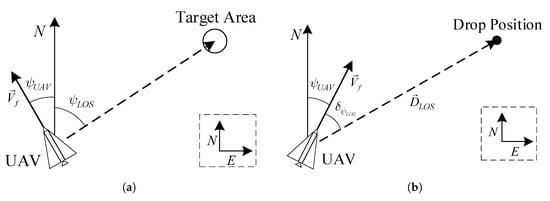
Figure 3.
Problems Description among UAV Airdrop Task: (a) the UAV should turn its nose towards target area firstly; (b) after adjustment of azimuth, the UAV could follow the guidance of UAV maneuver decision-making policy until reaching target position.
- Turn round problem: UAV flies from a random starting point and turns to the direction of target area demanded. During this process, pilots usually manipulate UAVs and controls the azimuth of UAVs towards target direction.
- Guidance problem: UAV starts from a random position and flies to a drop position given by commander. If the pilot want to manually finish this work, it will take lots of energy because the pilot should plan an effective path and manipulate the UAV following it.
If we want to simulate this process described above, a dynamical model of UAV should be constructed. We adopted a dynamical model describing airdrop task based on 3-DoF kinematic model of UAV [22]. When the position and attitude of UAV are confirmed at t, we can obtain the state of UAV at t+1 by solving the model we designed. Therefore, we think that the transition probability of UAV maneuver decision-making model is , which belongs to deterministic model.
Based on the 3-DoF kinematic model of UAV, the flight state is defined as , where is the horizontal coordinates of the UAV in the geographical coordinate system, and is the flight path azimuth Angle of the UAV. On the other hand, the steering overload of UAV is defined as , where represents the max normal acceleration of UAV in the body coordinate system. During the simulation process, algorithm outputs the current optimal maneuver control and the next state of UAV is calculated combined with the current state according to the flight simulation model of UAV.
2.1.3. State Representation and Action Design
Based on the problems’ definition among airdrop task, we can design the state space of two problems mentioned above separately. Specifically, action space is the same for both problems because the core kinematic model is all realized based on the 3-DoF kinematic model of UAV.
(1) State Space of Turn Round Problem
Considering that turn round problem is related to the azimuth of UAV and the relative direction of relative orientation between UAV and target area, we designed the state space of turn round problem, that is defined as
where is the relative azimuth between LOS and nose direction of UAV, and represents the steering overload of UAV. could be calculated by
where is the azimuth of LOS relative to North, and is the azimuth of UAV relative to North. Two symbols are all in and satisfy the right-hand rule.
(2) State Space of Guidance Problem
For the guidance problem of airdrop task, we can define its state space as
where indicates the distance between UAV and drop position. Moreover, if we define as the position of UAV and as the drop position, we will calculate the symbols by
where represents the 2-norm of vector.
(3) Action Space of Both Problems
Based on the flight simulation model of UAV we constructed, we can establish the action space as below.
2.1.4. Reward Function Based on Potential-Based Reward Shaping
In MDPs, the reward function determines the direction of policy iteration and directly reflects the agent’s intention. The termination condition of turn round problem can be defined as follows:
where is at decision moment t, and is the minimum error of . This termination condition means that, when the UAV heads to the target area with an error under certain tolerance, we could think that the turn round problem has been solved. Analogously, the termination condition of guidance problem could be also obtained as
where is at decision moment t, and is the minimum error of the distance between the UAV and the required drop position.
Therefore, the reward function of the problems could be defined as
Equation (11) indicates that if UAV’s state satisfies termination condition of problems, will return 1.0, otherwise 0.0.
The algorithm we proposed could search the optimal policy according to this kind of episodic reward, but there is a serious fault that is possible to influence the efficiency of policy convergence because the rewards environment returned are too sparse to learn useful experience, such as those samples whose reward is not zero. Thus, some researchers proposed the potential-based reward shaping [23,24] (PBRS) method to solve the problem brought by “sparse” reward. PBRS provides a guidance signal for improving the speed of policy convergence by adding a new reward shaping function to original reward function. Generally, should satisfy
where is a discount factor, and , , and indicate the current state, the current action, and the next state, respectively. Moreover, is a kind of potential energy function. If agent’s action help it approach termination condition, it will receive a positive reward, otherwise negation. In summary, traditional MDPs can be rewritten as
and new reward function is defined as
In the following, we present the shaping function for each individual problem.
(1) The Shaping Function for Turn Round Problem
Based on the definition of turn round problem, we can obtain the shaping function for turn round problem as shown in Equation (15).
In Equation (15), is the coefficient of azimuth error factor, and is the coefficient of maneuver factor.
(2) The Shaping Function for Guidance Problem
As shown in Equation (16), the definition of the shaping function of guidance problem is given.
In the equation, is distance that UAV approaches drop position after one simulation step, is the coefficient of distance factor. Moreover, T is simulation step, is the maximum speed of UAV. The symbol could be calculated by
where is the distance between UAV and drop position at t-th decision step.
2.2. The UAV Maneuver Decision-Making Algorithm for Autonomous Airdrop Based on Per-DDPG
2.2.1. The Framework of Per-DDPG
The Deep Deterministic Policy Gradient (DDPG) is a model-free, off-policy, and DRL-based algorithm based on Actor-Critic architecture. It can effectively solve problems belonging to MDPs with continuous state space and action space.
Although DDPG can avoid the dimensional explosion problem brought by continuous state space and action space, it does not consider the diversity of data and does not utilize historical experience fully. This results in the low convergence speed of DDPG’s policy and poor stability of the convergence result. Meanwhile, because the episode of UAV maneuver decision-making is short, while the task process lasts a long time, the changing of reward is not obvious. Thus, the value density of historical experience is low. That is the reason why we use PER to generate training data [17], which can improve the utilization of the potential value of historical experiences, thereby increasing convergence speed and enhancing the stability of training results.
Figure 4 shows the block diagram of the PER-DDPG’s structure. At each decision-making step, the actor network outputs action with noise for exploring according to state, and the current state, action, reward, and next state are packaged and stored in experience memory D. During the process of storing experience, samples bind with probability used for PER sampling. And then, the training data is sampled from D by PER, and every sampled data’s TD-error [25] between current and target value is calculated for updating the priority of data and being cumulated for updating network’s parameters with importance sampling (IS) weights. Finally, the parameters of main networks and are updated, and the parameters of target networks and are also updated smoothly because of stability of network training.
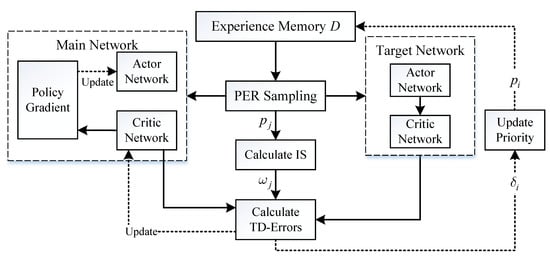
Figure 4.
The diagram of Prioritized Experience Replay-Deep Deterministic Policy Gradient (PER-DDPG)’s framework.
At each moment, the algorithm gives action by
where is the current state, and is the resulting output by the actor function . During the training process, the critic function evaluates current action given by actor function, and the evaluation is used for the basis of updating .
2.2.2. The UAV Maneuver Decision-Making Network
As mentioned above, DDPG is a kind of deep reinforcement learning algorithm based on the Actor-Critic framework. During the training process, the actor network outputs action according to state generated by environment. Meanwhile, TD-error is used to optimize the critic network and update its parameters. Similarly, the actor network’s parameters are optimized according to . Therefore, we must design the structure of actor and critic networks, respectively, on the basis of DL.
(1) Actor Network
The actor network is mainly used to output action in real-time decision according to state. The input vector of the network is the current state , and the output vector of the network is the current action calculated by . Considering the definition of state space, the dimension of network input is , and the dimension of output is . As shown in Figure 5, it is the normal structure of actor network .
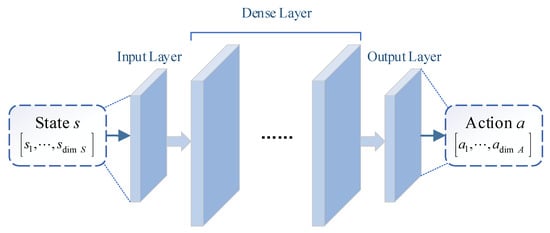
Figure 5.
The structure of actor network.
(2) Critic Network
The critic network is used to evaluate the advantage of current action output by . The network input is , and the network output is . According to state space and action space defined above, the dimension of network input is , and the dimension of network output is 1. As shown in Figure 6, it is the normal structure of critic network .
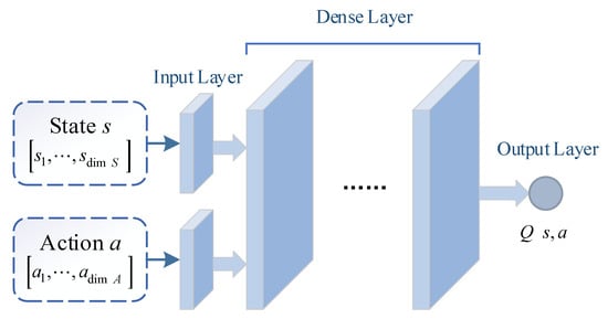
Figure 6.
The structure of critic network.
In addition, before state and action are entered into network, the value of input vector should be normalized for eliminating the influence of data’s physical meaning. Moreover, the structure of target networks and is similar to and , and only the method of parameters updating is distinguished.
2.2.3. The Training Procedure of UAV Maneuver Decision-Making Algorithm
Based on MDPs, the key issue of searching optimal UAV maneuver decision-making policy is to solve an optimization problem defined as
where is defined in Equation (3). In this paper, we use Double Q-Learning [18] to update the , as defined in Equation (20).
In the equation above, is current state, is current action, is current reward, is next state, and is the learning rate of the algorithm. As shown in Equation (21), it is loss function of critic network .
The symbol is TD-error based on Double Q-Learning of j-th data sampling from memory D. TD-error describes the difference between and optimal goal, and it is defined as
where is the optimal goal of , is j-th training data, and and are current state and action in , respectively. The symbol could be calculated by
where and are current reward and next state in . Thus, we can obtain the gradient of loss function as shown below considering Equations (21) and (22).
At the same time, we define the loss function of actor network in order to update the parameters of .
Thereby, we can obtain the gradient of according to deterministic policy gradient theorem [26], as shown in Equation (26).
During the process of training networks, we use the PER method to sample training data from D in order to utilize the diversity of experiences fully. Usually, the training data is sampled by selecting a batch of data from D uniformly, which means the probability of each sample selected in D is equal. On the contrary, of PER is not same, as defined as Equation (27).
In the equation above, is the priority of i-th sample in D, and is a hyperparameter. When , it is pure UER. is defined based on TD-error, as shown in Equation (28).
Among the equation above, is TD-error of i-th sample in D. Moreover, a minimum is introduced to prevent from being 0.
Although PER improves the availability of experiences, the distribution error of training data sampled by PER occurs compared with UER’s, and this problem also reduces the diversity of training samples. Therefore, importance sampling (IS) weights are introduced to correct the distribution error of training data caused by PER. The IS weight is defined as Equation (29).
In the equation above, N is the size of D. When , the distribution error of training set is fully compensated. When is calculated, the actual updating target is and it’s used to replace in Equation (24). Therefore, the final gradient of is calculated by
In order to ensure the stable convergence of the network, is normalized by . Thereby, the actual IS weight could be defined as
At the same time, in the early stage of training, the distribution error caused by PER is not big. Thus, we define an initial , and it gradually increases to 1 with training going on.
In addition, because of stability of target networks’ training, the parameters of and are updated by “Soft” updating similar to smooth updating, as shown in Equation (32).
In the equation above, the symbol is a hyperparameter involved in the “Soft” updating. Moreover, a kind of random noise is used to improve the exploration ability of deterministic policy involved in algorithm, as shown in Equation (33).
Among the equation, is a kind of time-variant noise. Because the UAV maneuver decision-making satisfies the Markovian condition and the changing of state is inertial process, an autocorrelation noise model called Ornstein Uhlenbeck (OU) process [27] is used for action exploration. The iterative formula of is shown in Equation (34).
In the equation above, and are current and next value of noise separately. and indicate the mean value and regression rate of noise, respectively. Moreover, is the step of noise, and represents the Wiener process.
Finally, the training procedure of UAV maneuver decision-making algorithm is given in Algorithm 1.
| Algorithm 1 The UAV Maneuver Decision-Making Algorithm for Airdrop Task. |
|
3. Results and Analysis
According to content aforementioned, we design some experiments to verify the availability of the algorithm we proposed and compare PER with UER in terms of the efficiency of policy optimization. In the following, we will explain the setting of simulation environment, training results, and results of Monte-Carlo (MC) test experiments, as well as their analysis.
3.1. The Settings of Simulation Environment
In the experiments we designed, the drop area and UAV are restricted to 100 km × 100 km airspace at the height of 5000 m. For each simulation experiment, the UAV’s initial state is randomly generated, and the UAV might start from arbitrary position in flight airspace. In order to make simulation closer to real environment, we decide to make s because UAV’s control input is usually updated by human pilot every 0.5 s ∼ 1 s.
Moreover, because each dimension of state space has different physical units, the state and action should be normalized before it’s input into and . As shown in Table 1, the details of data are explained. Thereby, we can normalize parameters according to their physical meanings.

Table 1.
The details of data input into networks.
3.2. The Simulation Results and Analysis of Turn Round Problem
3.2.1. The Parameters Setting of Algorithm
According to the training procedure of algorithm, before we start training, some parameters should be assigned. As shown in Table 2, there are some parameters assignments of algorithm. Moreover, we design the structure of networks and shown in Table 3 and Table 4, respectively, according to the state space and action space of turn round problem. In this paper, the networks are all designed by fully-connected neural network, which means the layers are dense layers.
Table 2.
The parameters assignment of algorithm.
Table 3.
The structure of critic network .
Table 4.
The structure of actor network .
3.2.2. The Analysis of Simulation Results
Based on the setting above, we finished the training of networks successfully and the loss diagrams of critic networks involved in UER-DDPG and PER-DDPG over time are shown in Figure 7, respectively. We could find that the loss of PER-DDPG converges faster than UER-DDPG. Moreover, the loss of PER-DDPG becomes stable after converging to minimum. On the contrary, when UER-DDPG converges, the loss fluctuated greatly at 1000th episode, and its convergence costs more time.
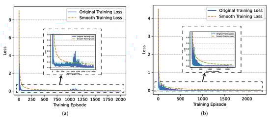
Figure 7.
The comparison of critic networks’ training loss involved in Uniform Experience Replay (UER)-DDPG and PER-DDPG over training episode. (a) The training loss of critic network of UER-DDPG. (b) The training loss of critic network of PER-DDPG.
Figure 8 is the winning rate of algorithms based on different experience replay methods over simulation episode during the training process. We can find that all the winning rates are more than and maintain stably. It is shown that DDPG with PER method could achieve the same result compared with UER-DDPG. But the training process of PER-DDPG is much stabler than UER-DDPG because the winning rate of UER-DDPG fluctuates violently at the beginning of training. Meanwhile, the curve of episode rewards further demonstrates that PER-DDPG is much steadier than UER-DDPG from Figure 9.
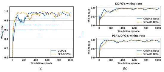
Figure 8.
The winning rate of algorithms based on UER-DDPG and PER-DDPG over simulation episode. Winning rate means a rate of finishing mission successfully. (a) The comparison of winning rate based on UER-DDPG and PER-DDPG. (b) The top figure is the winning rate of algorithm based on UER-DDPG, and the figure at the bottom is the winning rate of algorithm based on PER-DDPG.
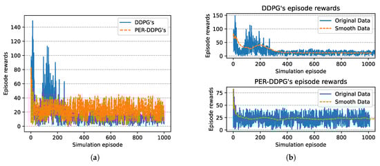
Figure 9.
The episode rewards of algorithms based on UER-DDPG and PER-DDPG over simulation episode. (a) The comparison of episode rewards based on UER-DDPG and PER-DDPG. (b) The top figure is the episode rewards of algorithm based on UER-DDPG, and the bottom figure is the episode rewards of algorithm based on PER-DDPG.
After training, we run a group of Monte-Carlo experiments for trained results of UER-DDPG and PER-DDPG, and the number of MC experiments for each result is 1000. As shown in Table 5, the training result’s performance of PER-DDPG is better than UER-DDPG’s because the winning rate of PER-DDPG’s is more than about than UER-DDPG’s. Meanwhile, we visualize some typical test results from MC experiments, and Figure 10, Figure 11, Figure 12 and Figure 13 is the flight trajectory of UAV and some parameters, including azimuth, reward, and action, over simulation step.
Table 5.
The analysis of MC experiments for the trained results of UER-DDPG and PER-DDPG.
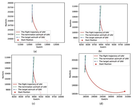
Figure 10.
The flight trajectory from Monte-Carlo (MC) experiments for the trained result of UER-DDPG: (a) the flight trajectory of 1st experiment; (b) the flight trajectory of 2nd experiment; (c) the flight trajectory of 3rd experiment; (d) the flight trajectory of 4th experiment.
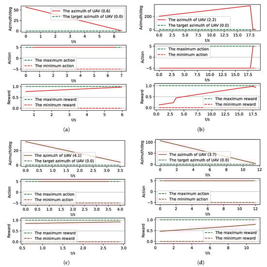
Figure 11.
The parameters curve from MC experiments for the trained result of UER-DDPG. (a) The parameters curve of 1st experiment; (b) the parameters curve of 2nd experiment; (c) the parameters curve of 3rd experiment; (d) the parameters curve of 4th experiment.
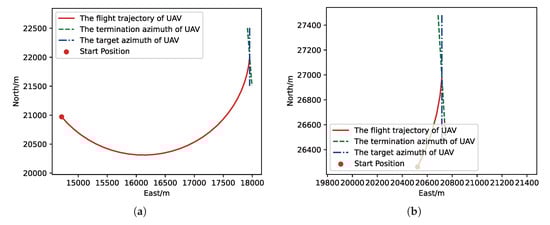
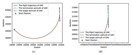
Figure 12.
The flight trajectory from MC experiments for the trained result of PER-DDPG: (a) the flight trajectory of 1st experiment; (b) the flight trajectory of 2nd experiment; (c) the flight trajectory of 3rd experiment; (d) the flight trajectory of 4th experiment.
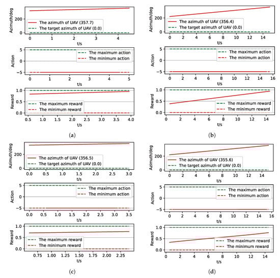
Figure 13.
The parameters curve from MC experiments for the trained result of PER-DDPG: (a) The parameters curve of 1st experiment. (b) The parameters curve of 2nd experiment. (c) The parameters curve of 3rd experiment. (d) The parameters curve of 4th experiment.
In Figure 10 and Figure 12 the red solid line represents the flight trajectory of UAV, and the red dashed line and the blue dash dot line indicate the termination azimuth of UAV and the required azimuth of LOS. In Figure 11 and Figure 13, the 1st row each figure is azimuth of UAV over simulation step, the 2nd row each figure is action of UAV over simulation step, and the 3rd row each figure is reward of UAV received over simulation step.
We can find that the algorithm based on PER-DDPG we proposed solves the turn round problem involved in airdrop task, and its performance is more than UER-DDPG. In summary, not only is the training process of algorithm based on PER-DDPG stabler than UER-DDPG’s, but also the trained result of algorithm based on PER-DDPG is much more effective than UER-DDPG’s.
3.3. The Simulation Results and Analysis of Guidance Problem
3.3.1. The Parameters Setting of Algorithm
Based on content above, there are some parameters assignments of algorithm for guidance problem shown in Table 6. Moreover, according to the state space and action space of guidance problem, the structure of networks and is shown in Table 7 and Table 8, respectively.
Table 6.
The parameters assignment of algorithm.
Table 7.
The structure of critic network .
Table 8.
The structure of actor network .
3.3.2. The Analysis of Simulation Results
Similarly, we also analyzed the training loss, the winning rate, and the episode rewards generated during the training process of algorithms. In Figure 14, we could find that the convergence speed of PER-DDPG is more than UER-DDPG’s due to high utilization of experiences, and PER-DDPG becomes much stabler than UER-DDPG because the fluctuation of PER-DDPG is less than UER-DDPG.
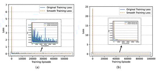
Figure 14.
The comparison of critic networks’ training loss involved in UER-DDPG and PER-DDPG over training episode. (a) The training loss of critic network of UER-DDPG. (b) The training loss of critic network of PER-DDPG.
In Figure 15, the winning rate of algorithms based on different experience replay methods over simulation episode during the training process is shown. We can find that the winning rate curves of UER-DDPG and PER-DDPG are stable after some simulation episodes and maintain a high value. And the winning rate of PER-DDPG is much more than UER-DDPG after fluctuation. Meanwhile, the comparison of episode rewards could demonstrate that PER-DDPG is much steadier than UER-DDPG because the fluctuation of episode rewards of PER-DDPG is clearly less than UER-DDPG from Figure 16.
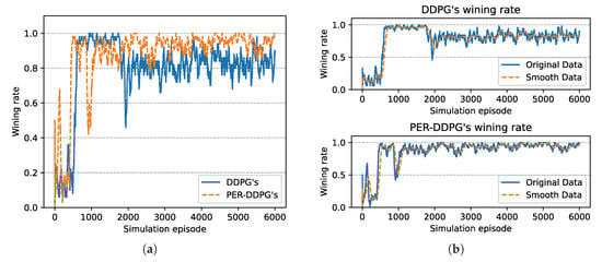
Figure 15.
The winning rate of algorithms based on UER-DDPG and PER-DDPG over simulation episode. Winning rate means a rate of finishing mission successfully. (a) The comparison of winning rate based on UER-DDPG and PER-DDPG. (b) The figure in 1st row is the winning rate of algorithm based on UER-DDPG, and the figure in 2nd row is the winning rate of algorithm based on PER-DDPG.
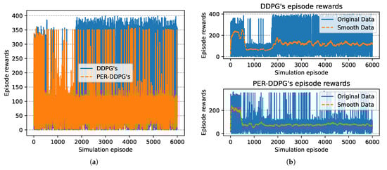
Figure 16.
The episode rewards of algorithms based on UER-DDPG and PER-DDPG over simulation episode. The legends of figure are the same to Figure 9. (a) The comparison of episode rewards based on UER-DDPG and PER-DDPG. (b) The figure in 1st row is the episode rewards of algorithm based on UER-DDPG, and the figure in 2nd row is the episode rewards of algorithm based on PER-DDPG.
After training, we finished a set of Monte-Carlo experiments for trained results of UER-DDPG and PER-DDPG, and the number of it for each result is 1000. As shown in Table 9, the winning rate of PER-DDPG is more than approximately than PER-DDPG, and we can think that the training result’s performance of PER-DDPG is better than UER-DDPG’s.
Table 9.
The analysis of Monte-Carlo (MC) experiments for the trained results of UER-DDPG and PER-DDPG.
Moreover, we visualize some typical test results from MC experiments in order to make our analysis more convincing. Figure 17, Figure 18, Figure 19 and Figure 20 is the flight trajectory of UAV and some parameters, including reward and action over simulation step. In Figure 17 and Figure 19, the red solid line represents the flight trajectory of UAV, and the blue dashed circle represents the maximum range of drop area. The red solid point and green solid point indicate start position and drop position. In Figure 18 and Figure 20, the top figure is the action of UAV over simulation step, the bottom figure is the reward of UAV received over simulation step.
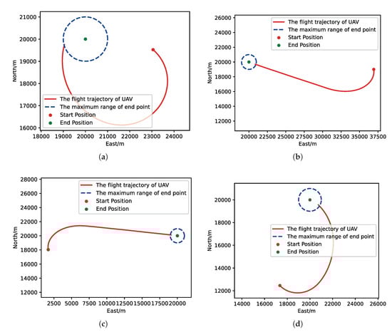
Figure 17.
The flight trajectory from MC experiments for the trained result of UER-DDPG: (a) The flight trajectory of 1st experiment. (b) The flight trajectory of 2nd experiment. (c) The flight trajectory of 3rd experiment. (d) The flight trajectory of 4th experiment.
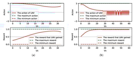
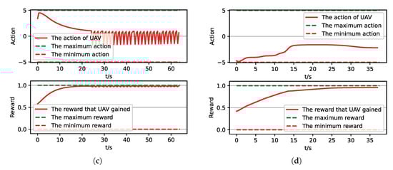
Figure 18.
The parameters curve from MC experiments for the trained result of UER-DDPG. (a) The parameters curve of 1st experiment. (b) The parameters curve of 2nd experiment. (c) The parameters curve of 3rd experiment. (d) The parameters curve of 4th experiment.
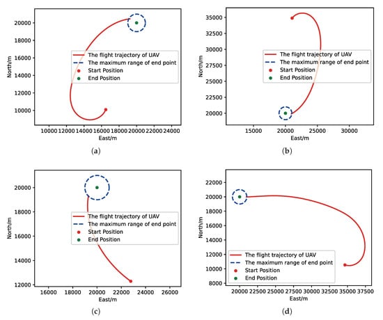
Figure 19.
The flight trajectory from MC experiments for the trained result of PER-DDPG: (a) The flight trajectory of 1st experiment. (b) The flight trajectory of 2nd experiment. (c) The flight trajectory of 3rd experiment. (d) The flight trajectory of 4th experiment.
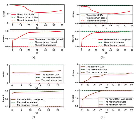
Figure 20.
The parameters curve from MC experiments for the trained result of PER-DDPG: (a) The parameters curve of 1st experiment. (b) The parameters curve of 2nd experiment. (c) The parameters curve of 3rd experiment. (d) The parameters curve of 4th experiment.
According to results and analysis above, we could find that the algorithm based on PER-DDPG we proposed solves the guidance problem involved in airdrop task, and its performance is more than UER-DDPG. Similarly, not only is the training process of algorithm based on PER-DDPG stabler than UER-DDPG’s, but also the trained result of algorithm based on PER-DDPG is much more effective than UER-DDPG’s, while solving the guidance problem.
4. Conclusions
Aiming at the airdrop task, we refined and described two key issues, including turn round problem and guidance problem. Based on the definitions of problems, we designed the UAV maneuver decision-making model for airdrop task based on MDPs and constructed the state space, the action space, and the reward function based on PBRS. Then, we proposed the UAV maneuver decision-making algorithm for autonomous airdrop based on Deep Reinforcement Learning. Particularly, we used Prioritized Experience Replay to improve the availability of experiences during training process. Meanwhile, the results showed that the algorithm we proposed could be able to solve the turn round problem and guidance problem after training successfully. And the convergence of PER-DDPG is faster and stabler than UER-DDPG and the trained result performance of PER-DDPG is also better than UER-DDPG. In the future, we will investigate the solution of UAV autonomous flight when state is partially observed. And we will extend the algorithm we proposed to manipulate the real UAV to improve the autonomy of UAV, while performing special missions in the real world.
Author Contributions
Conceptualization, K.Z.; methodology, K.L. and K.Z.; software, K.L., K.Z., Z.Z., Z.L. and S.H.; validation, K.L. and K.Z.; formal analysis, S.H.; resources, K.Z. and J.H.; writing—original draft preparation, K.L.; writing—review and editing, K.L.; visualization, Z.Z. and Z.L.; supervision, K.Z.; funding acquisition, K.Z. All authors have read and agreed to the published version of the manuscript.
Funding
This research was funded by the Natural Science Basic Research Program of Shaanxi Program grant number No.2020JM-147, the seed Foundation of Innovation and Creation for Graduate Students in Northwestern Polytechnical University grant number ZZ2019021, the Key Laboratory Project Foundation grant number 6142504190105.
Institutional Review Board Statement
Not applicable.
Informed Consent Statement
Not applicable.
Acknowledgments
We would like to thank Xiaodong Cheng (Cambridge University) for insightful discussions and valuable suggestions.
Conflicts of Interest
The authors declare no conflict of interest.
References
- Menouar, H.; Guvenc, I.; Akkaya, K.; Uluagac, A.S.; Kadri, A.; Tuncer, A. UAV-enabled intelligent transportation systems for the smart city: Applications and challenges. IEEE Commun. Mag. 2017, 55, 22–28. [Google Scholar] [CrossRef]
- Mathisen, S.G.; Leira, F.S.; Helgesen, H.H.; Gryte, K.; Johansen, T.A. Autonomous ballistic airdrop of objects from a small fixed-wing unmanned aerial vehicle. Auton. Robot. 2020, 44, 859–875. [Google Scholar] [CrossRef]
- Klinkmueller, K.; Wieck, A.; Holt, J.; Valentine, A.; Bluman, J.E.; Kopeikin, A.; Prosser, E. Airborne delivery of unmanned aerial vehicles via joint precision airdrop systems. In Proceedings of the AIAA Scitech 2019 Forum, San Diego, CA, USA, 7–11 January 2019; p. 2285. [Google Scholar]
- Yang, L.; Qi, J.; Xiao, J.; Yong, X. A literature review of UAV 3D path planning. In Proceedings of the 11th World Congress on Intelligent Control and Automation, Shenyang, China, 29 June–4 July 2014; pp. 2376–2381. [Google Scholar]
- Huang, S.; Teo, R.S.H. Computationally efficient visibility graph-based generation of 3D shortest collision-free path among polyhedral obstacles for unmanned aerial vehicles. In Proceedings of the 2019 International Conference on Unmanned Aircraft Systems (ICUAS), Atlanta, GA, USA, 11–14 June 2019; pp. 1218–1223. [Google Scholar]
- Cheng, X.; Zhou, D.; Zhang, R. New method for UAV online path planning. In Proceedings of the 2013 IEEE International Conference on Signal Processing, Communication and Computing (ICSPCC 2013), KunMing, China, 5–8 August 2013; pp. 1–5. [Google Scholar]
- Sun, Q.; Li, M.; Wang, T.; Zhao, C. UAV path planning based on improved rapidly-exploring random tree. In Proceedings of the 2018 Chinese Control and Decision Conference (CCDC), Shenyang, China, 9–11 June 2018; pp. 6420–6424. [Google Scholar]
- Yan, F.; Liu, Y.S.; Xiao, J.Z. Path planning in complex 3D environments using a probabilistic roadmap method. Int. J. Autom. Comput. 2013, 10, 525–533. [Google Scholar] [CrossRef]
- Tseng, F.H.; Liang, T.T.; Lee, C.H.; Der Chou, L.; Chao, H.C. A star search algorithm for civil UAV path planning with 3G communication. In Proceedings of the 2014 Tenth International Conference on Intelligent Information Hiding and Multimedia Signal Processing, Kitakyushu, Japan, 27–29 August 2014; pp. 942–945. [Google Scholar]
- Meng, B.B.; Gao, X. UAV path planning based on bidirectional sparse A* search algorithm. In Proceedings of the 2010 International Conference on Intelligent Computation Technology and Automation, Changsha, China, 11–12 May 2010; Volume 3, pp. 1106–1109. [Google Scholar]
- Zhang, Z.; Wu, J.; Dai, J.; He, C. A novel real-time penetration path planning algorithm for stealth UAV in 3D complex dynamic environment. IEEE Access 2020, 8, 122757–122771. [Google Scholar] [CrossRef]
- Silva Arantes, J.D.; Silva Arantes, M.D.; Motta Toledo, C.F.; Júnior, O.T.; Williams, B.C. Heuristic and genetic algorithm approaches for UAV path planning under critical situation. Int. J. Artif. Intell. Tools 2017, 26, 1760008. [Google Scholar] [CrossRef]
- Kaminer, I.; Pascoal, A.; Hallberg, E.; Silvestre, C. Trajectory tracking for autonomous vehicles: An integrated approach to guidance and control. J. Guid. Control. Dyn. 1998, 21, 29–38. [Google Scholar] [CrossRef]
- Lee, H.; Kim, H.J. Trajectory tracking control of multirotors from modelling to experiments: A survey. Int. J. Control Autom. Syst. 2017, 15, 281–292. [Google Scholar] [CrossRef]
- Mnih, V.; Kavukcuoglu, K.; Silver, D.; Rusu, A.A.; Veness, J.; Bellemare, M.G.; Graves, A.; Riedmiller, M.; Fidjeland, A.K.; Ostrovski, G.; et al. Human-level control through deep reinforcement learning. Nature 2015, 518, 529–533. [Google Scholar] [CrossRef] [PubMed]
- Lillicrap, T.P.; Hunt, J.J.; Pritzel, A.; Heess, N.; Erez, T.; Tassa, Y.; Silver, D.; Wierstra, D. Continuous control with deep reinforcement learning. arXiv 2015, arXiv:1509.02971. [Google Scholar]
- Schaul, T.; Quan, J.; Antonoglou, I.; Silver, D. Prioritized experience replay. arXiv 2015, arXiv:1511.05952. [Google Scholar]
- Van Hasselt, H.; Guez, A.; Silver, D. Deep reinforcement learning with double q-learning. In Proceedings of the AAAI Conference on Artificial Intelligence, Phoenix, AZ, USA, 12–17 February 2016; Volume 30. [Google Scholar]
- Hou, Y.; Liu, L.; Wei, Q.; Xu, X.; Chen, C. A novel DDPG method with prioritized experience replay. In Proceedings of the 2017 IEEE International Conference on Systems, Man, and Cybernetics (SMC), Banff, AB, Canada, 5–8 October 2017; pp. 316–321. [Google Scholar]
- Ragi, S.; Chong, E.K. UAV path planning in a dynamic environment via partially observable Markov decision process. IEEE Trans. Aerosp. Electron. Syst. 2013, 49, 2397–2412. [Google Scholar] [CrossRef]
- François-Lavet, V.; Henderson, P.; Islam, R.; Bellemare, M.G.; Pineau, J. An introduction to deep reinforcement learning. arXiv 2018, arXiv:1811.12560. [Google Scholar]
- Zhang, K.; Li, K.; He, J.; Shi, H.; Wang, Y.; Niu, C. A UAV Autonomous Maneuver Decision-Making Algorithm for Route Guidance. In Proceedings of the 2020 International Conference on Unmanned Aircraft Systems (ICUAS), Athens, Greece, 1–4 September 2020; pp. 17–25. [Google Scholar]
- Ng, A.Y.; Harada, D.; Russell, S. Policy invariance under reward transformations: Theory and application to reward shaping. In Proceedings of the Sixteenth International Conference on Machine Learning, Bled, Slovenia, 27–30 June 1999; Volume 99, pp. 278–287. [Google Scholar]
- Badnava, B.; Mozayani, N. A new potential-based reward shaping for reinforcement learning agent. arXiv 2019, arXiv:1902.06239. [Google Scholar]
- Tesauro, G. Temporal difference learning and TD-Gammon. Commun. ACM 1995, 38, 58–68. [Google Scholar] [CrossRef]
- Silver, D.; Lever, G.; Heess, N.; Degris, T.; Wierstra, D.; Riedmiller, M. Deterministic policy gradient algorithms. In Proceedings of the International Conference on Machine Learning, Beijing, China, 22–24 June 2014; pp. 387–395. [Google Scholar]
- Barndorff-Nielsen, O.E.; Shephard, N. Non-Gaussian Ornstein–Uhlenbeck-based models and some of their uses in financial economics. J. R. Stat. Soc. Ser. B 2001, 63, 167–241. [Google Scholar] [CrossRef]


Publisher’s Note: MDPI stays neutral with regard to jurisdictional claims in published maps and institutional affiliations. |
© 2021 by the authors. Licensee MDPI, Basel, Switzerland. This article is an open access article distributed under the terms and conditions of the Creative Commons Attribution (CC BY) license (http://creativecommons.org/licenses/by/4.0/).