
Do Radiographic Assessments of Periodontal Bone Loss Improve with Deep Learning Methods for Enhanced Image Resolution?


Abstract
1. Introduction
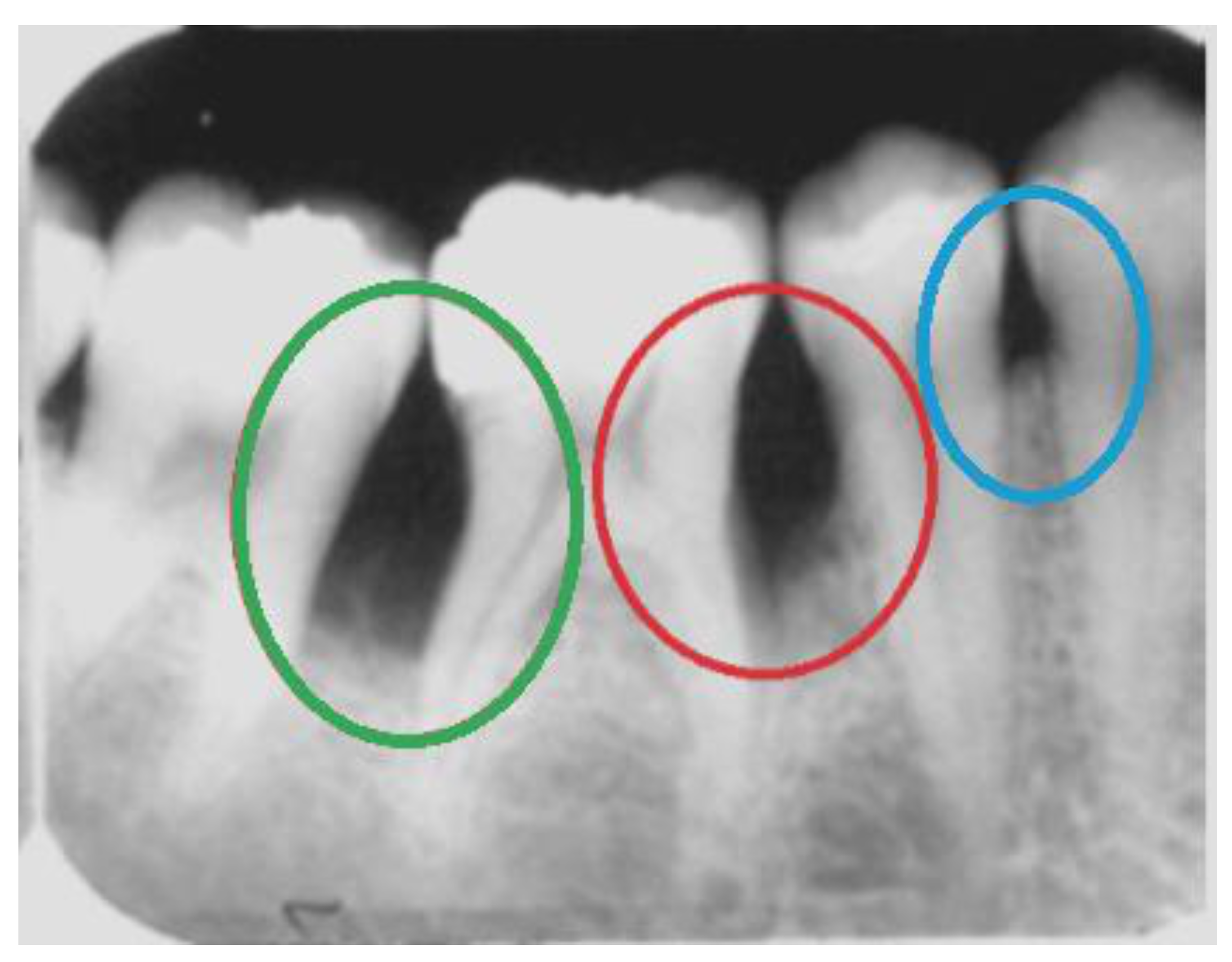
2. Radiographic Identification of Periodontal Bone Loss
Convolutional Neural Networks for PBL Identification
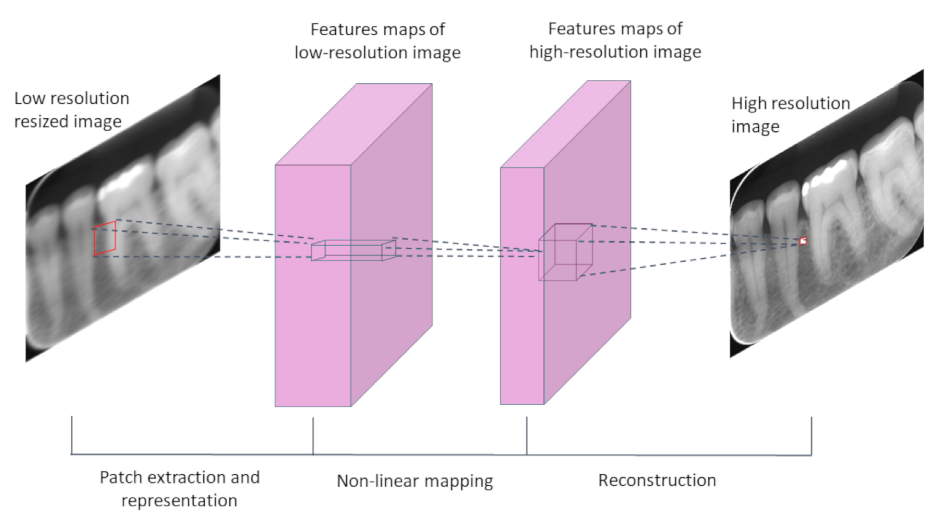
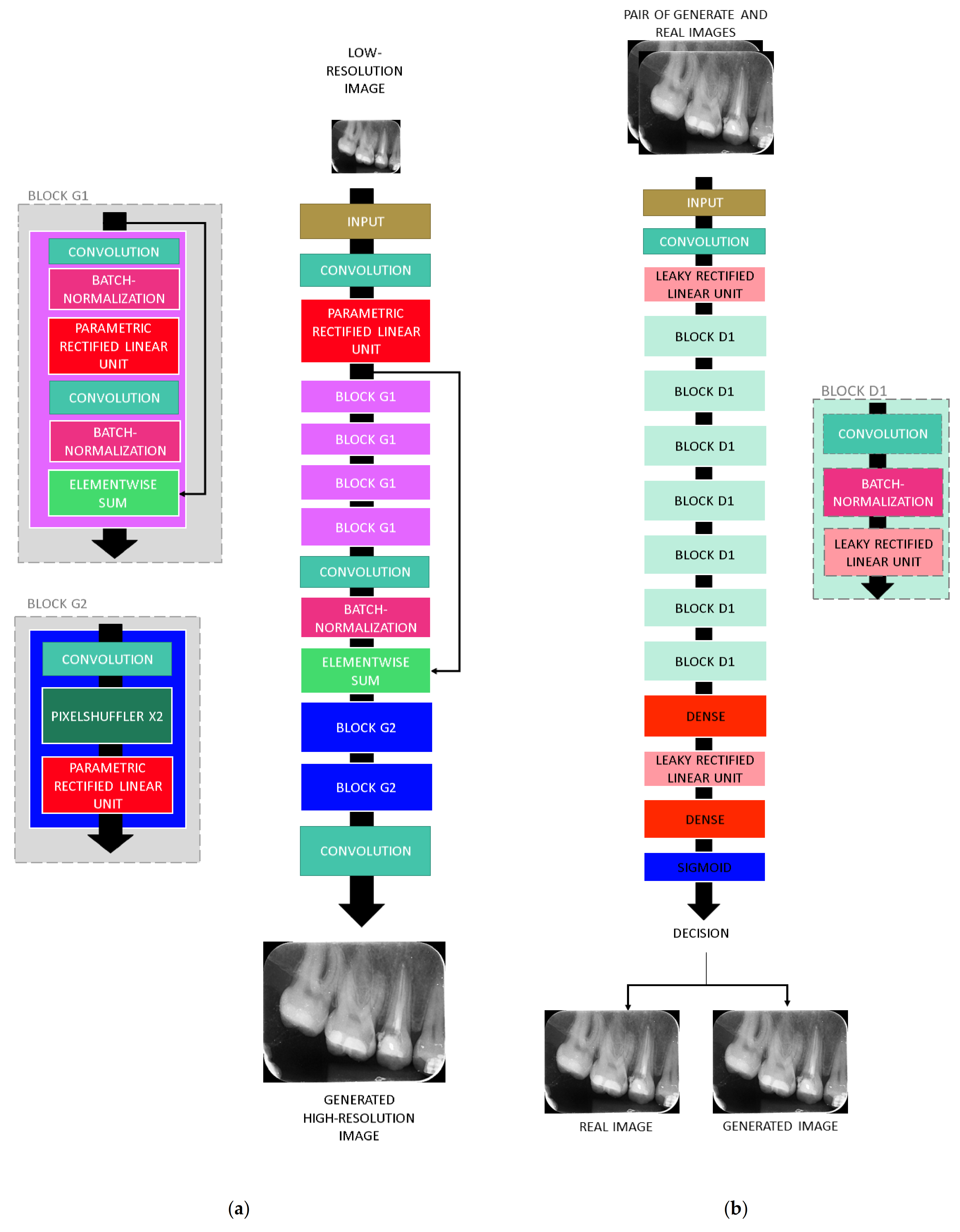
3. Deep-Learning Resolution Improvement Methods
4. Materials and Methods
4.1. Study 1—Qualitative Analysis of Image Quality
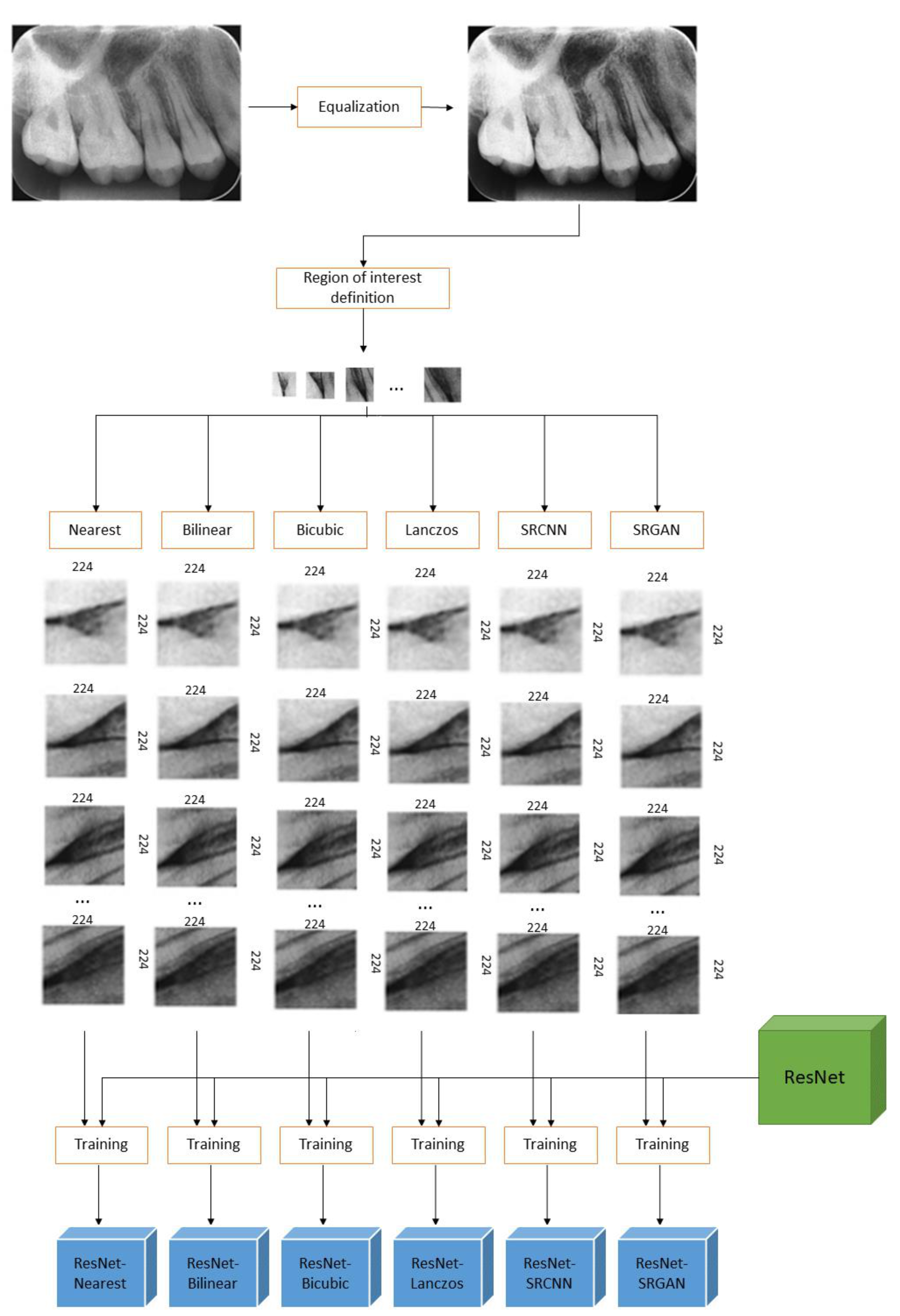
4.2. Study 2—Evaluation of the Impacts of Pre-Processing on Deep-Learning Based Classification
5. Results
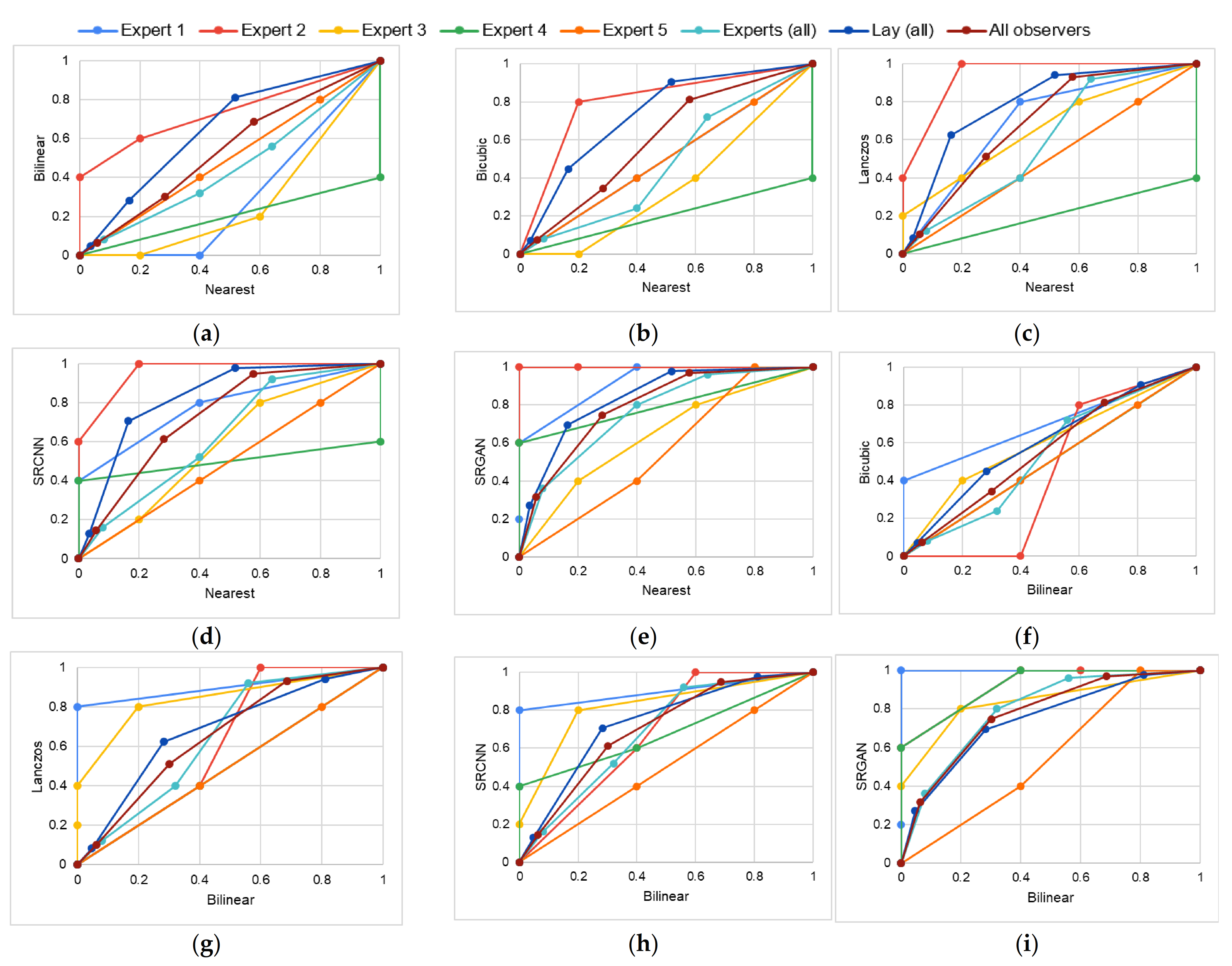
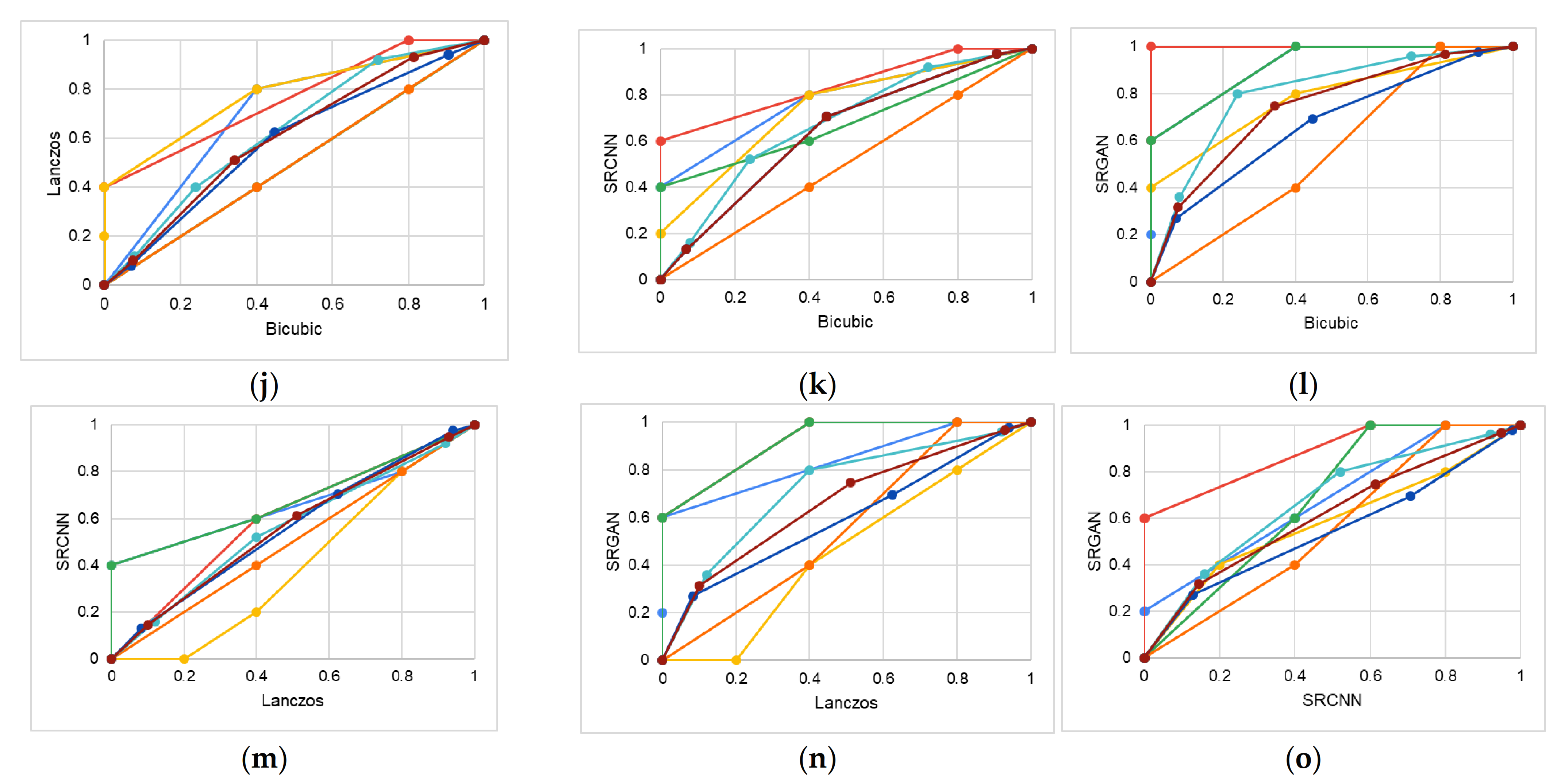
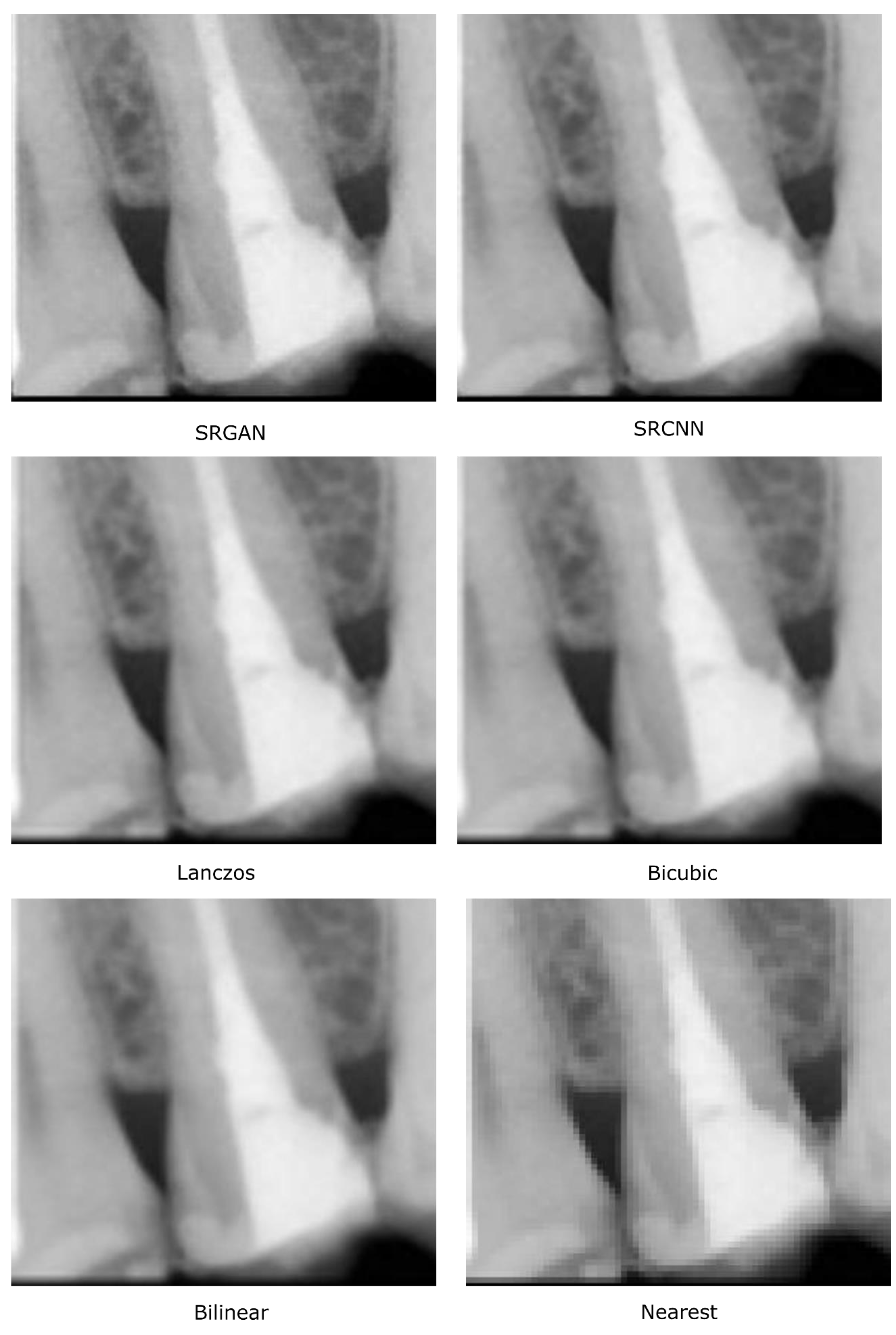
5.1. Study 1
5.2. Study 2
- True negatives (TN)—regions correctly classified as healthy;
- True positives (TP)—regions correctly classified as regions with bone loss;
- False negatives (FN)—regions with bone loss incorrectly classified as healthy;
- False positives (FP)—healthy regions incorrectly classified as regions with bone loss.
6. General Discussion
7. Conclusions
Author Contributions
Funding
Institutional Review Board Statement
Informed Consent Statement
Data Availability Statement
Acknowledgments
Conflicts of Interest
References
- Jeffcoat, M.K.; Wang, I.C.; Reddy, M.S. Radiographic Diagnosis in Periodontics. Periodontol. 2000 1995, 7, 54–68. [Google Scholar] [CrossRef]
- Tugnait, A.; Clerehugh, V.; Hirschmann, P.N. The Usefulness of Radiographs in Diagnosis and Management of Periodontal Diseases: A Review. J. Dent. 2000, 28, 219–226. [Google Scholar] [CrossRef]
- Estrela, C.; Bueno, M.R.; Leles, C.R.; Azevedo, B.; Azevedo, J.R. Accuracy of Cone Beam Computed Tomography and Panoramic and Periapical Radiography for Detection of Apical Periodontitis. J. Endod. 2008, 34, 273–279. [Google Scholar] [CrossRef] [PubMed]
- Tugnait, A.; Clerehugh, V.; Hirschmann, P.N. Survey of Radiographic Practices for Periodontal Disease in UK and Irish Dental Teaching Hospitals. Dentomaxillofac Radiol 2000, 29, 376–381. [Google Scholar] [CrossRef]
- Douglass, C.W.; Valachovic, R.W.; Wijesinha, A.; Chauncey, H.H.; Kapur, K.K.; McNeil, B.J. Clinical Efficacy of Dental Radiography in the Detection of Dental Caries and Periodontal Diseases. Oral Surg. Oral Med. Oral Pathol. 1986, 62, 330–339. [Google Scholar] [CrossRef]
- Pepelassi, E.A.; Diamanti-Kipioti, A. Selection of the Most Accurate Method of Conventional Radiography for the Assessment of Periodontal Osseous Destruction. J. Clin. Periodontol 1997, 24, 557–567. [Google Scholar] [CrossRef]
- Rohlin, M.; Akesson, L.; Hakansson, J.; Hakansson, H.; Nasstrom, K. Comparison between Panoramic and Periapical Radiography in the Diagnosis of Periodontal Bone Loss. Dentomaxillofacial Radiol. 1989, 18, 72–76. [Google Scholar] [CrossRef] [PubMed]
- Krois, J.; Ekert, T.; Meinhold, L.; Golla, T.; Kharbot, B.; Wittemeier, A.; Schwendicke, F. Deep Learning for the Radiographic Detection of Periodontal Bone Loss. Sci. Rep. 2019, 9, 1–6. [Google Scholar] [CrossRef]
- Faria, M.D.B. Quantitative Analysis of Radiation Dose for Critical Organs during Linear Tomography Regarding Intraosseous Dental Implant Planning. Master’s Thesis, Universidade Estadual de Campinas, Campinas, Brazil, 1997. [Google Scholar]
- Baskan, O.; Erol, C.; Ozbek, H.; Paksoy, Y. Effect of Radiation Dose Reduction on Image Quality in Adult Head CT with Noise-Suppressing Reconstruction System with a 256 Slice MDCT. J. Appl. Clin. Med Phys. 2015, 16, 285–296. [Google Scholar] [CrossRef]
- De Morais, J.; Sakakura, C.; Loffredo, L.; Scaf, G. Accuracy of Zoomed Digital Image in the Detection of Periodontal Bone Defect: In Vitro Study. Dentomaxillofacial Radiol. 2006, 35, 139–142. [Google Scholar] [CrossRef]
- Kositbowornchai, S.; Basiw, M.; Promwang, Y.; Moragorn, H.; Sooksuntisakoonchai, N. Accuracy of Diagnosing Occlusal Caries Using Enhanced Digital Images. Dentomaxillofacial Radiol. 2004, 33, 236–240. [Google Scholar] [CrossRef]
- Alvares, H. D Analysis of the Impact of Image Interpolation Methods in the Segmentation of Skin Lesions Using the SegNet Convolutional Neural Network. Universidade Federal de Ouro Preto: Ouro Preto, Brazil, 2019. [Google Scholar]
- Goodfellow, I.; Bengio, Y.; Courville, A. Deep Learning (Adaptive Computation and Machine Learning); The MIT Press: Cambridge, MA, USA, 2016; ISBN 978-0-262-03561-3. [Google Scholar]
- Dodge, S.; Karam, L. Understanding How Image Quality Affects Deep Neural Networks. In Proceedings of the 8th International Conference on Quality of Multimedia Experience (QoMEX), Lisbon, Portugal, 6–8 June 2016; pp. 1–6. [Google Scholar]
- Koziarski, M.; Cyganek, B. Impact of Low Resolution on Image Recognition with Deep Neural Networks: An Experimental Study. Int. J. Appl. Math. Comput. Sci. 2018, 28, 735–744. [Google Scholar] [CrossRef]
- Chatfield, K.; Simonyan, K.; Vedaldi, A.; Zisserman, A. Return of the Devil in the Details: Delving Deep into Convolutional Nets. In Proceedings of the British Machine Vision Conference 2014, Nottingham, UK, 1–5 September 2014. [Google Scholar]
- Szegedy, C.; Wei, L.; Yangqing, J.; Sermanet, P.; Reed, S.; Anguelov, D.; Erhan, D.; Vanhoucke, V.; Rabinovich, A. Going Deeper with Convolutions. In Proceedings of the 2015 IEEE Conference on Computer Vision and Pattern Recognition (CVPR), Boston, MA, USA, 8–12 June 2015; pp. 1–9. [Google Scholar]
- Simonyan, K.; Zisserman, A. Very Deep Convolutional Networks for Large-Scale Image Recognition. arXiv 2014, arXiv:1409.1556. [Google Scholar]
- Krizhevsky, A.; Sutskever, I.; Hinton, G.E. ImageNet Classification with Deep Convolutional Neural Networks. Commun. Acm. 2017, 60, 84–90. [Google Scholar] [CrossRef]
- Moran, M.B.H.; Faria, M.D.B.; Giraldi, G.A.; Bastos, L.F.; Conci, A. Using Super-Resolution Generative Adversarial Network Models and Transfer Learning to Obtain High Resolution Digital Periapical Radiographs. Comput. Biol. Med. 2021, 129, 104139. [Google Scholar] [CrossRef] [PubMed]
- Zeng, K.; Zheng, H.; Cai, C.; Yang, Y.; Zhang, K.; Chen, Z. Simultaneous Single- and Multi-Contrast Super-Resolution for Brain MRI Images Based on a Convolutional Neural Network. Comput. Biol. Med. 2018, 99, 133–141. [Google Scholar] [CrossRef] [PubMed]
- Zhang, Y.; An, M. Deep Learning- and Transfer Learning-Based Super Resolution Reconstruction from Single Medical Image. J. Healthc. Eng. 2017, 2017, 1–20. [Google Scholar] [CrossRef]
- Hatvani, J.; Basarab, A.; Tourneret, J.-Y.; Gyongy, M.; Kouame, D. A Tensor Factorization Method for 3-D Super Resolution with Application to Dental CT. IEEE Trans. Med. Imaging 2019, 38, 1524–1531. [Google Scholar] [CrossRef]
- Umehara, K.; Ota, J.; Ishida, T. Application of Super-Resolution Convolutional Neural Network for Enhancing Image Resolution in Chest CT. J. Digit. Imaging 2018, 31, 441–450. [Google Scholar] [CrossRef]
- Park, J.; Hwang, D.; Kim, K.Y.; Kang, S.K.; Kim, Y.K.; Lee, J.S. Computed Tomography Super-Resolution Using Deep Convolutional Neural Network. Phys. Med. Biol. 2018, 63, 145011. [Google Scholar] [CrossRef]
- Båth, M.; Zachrisson, S.; Månsson, L.G. VGC Analysis: Application of the ROC Methodology to Visual Grading Tasks. In Proceedings of the Medical Imaging 2008: Image Perception, Observer Performance, and Technology Assessment, San Diego, CA, USA, 16–21 February 2008; p. 69170X. [Google Scholar]
- Perschbacher, S. Periodontal Diseases. In Oral Radiology: Principles and Interpretation; Elsevier: New York, NY, USA, 2014; pp. 299–313. [Google Scholar]
- Moran, M.B.H.; Faria, M.D.B.; Giraldi, G.A.; Bastos, L.F.; Inacio, B.; Conci, A. On Using Convolutional Neural Networks to Classify Periodontal Bone Destruction in Periapical Radiographs. In Proceedings of the 2020 IEEE International Conference on Bioinformatics and Biomedicine (BIBM), Seoul, Korea, 16–19 December 2020. [Google Scholar]
- Lin, P.L.; Huang, P.Y.; Huang, P.W. Automatic Methods for Alveolar Bone Loss Degree Measurement in Periodontitis Periapical Radiographs. Comput. Methods Programs Biomed. 2017, 148, 1–11. [Google Scholar] [CrossRef] [PubMed]
- Lee, J.-H.; Kim, D.; Jeong, S.-N.; Choi, S.-H. Diagnosis and Prediction of Periodontally Compromised Teeth Using a Deep Learning-Based Convolutional Neural Network Algorithm. J. Periodontal Implant. Sci. 2018, 48, 114. [Google Scholar] [CrossRef]
- Carmody, D.P.; McGrath, S.P.; Dunn, S.M.; van der Stelt, P.F.; Schouten, E. Machine Classification of Dental Images with Visual Search. Acad. Radiol. 2001, 8, 1239–1246. [Google Scholar] [CrossRef]
- Mol, A.; van der Stelt, P.F. Application of Computer-Aided Image Interpretation to the Diagnosis of Periapical Bone Lesions. Dentomaxillofacial Radiol. 1992, 21, 190–194. [Google Scholar] [CrossRef]
- Ekert, T.; Krois, J.; Meinhold, L.; Elhennawy, K.; Emara, R.; Golla, T.; Schwendicke, F. Deep Learning for the Radiographic Detection of Apical Lesions. J. Endod. 2019, 45, 917–922.e5. [Google Scholar] [CrossRef]
- Yang, C.-Y.; Ma, C.; Yang, M.-H. Single-Image Super-Resolution: A Benchmark. In Proceedings of the Computer Vision–ECCV 2014, Zürich, Switzerland, 6–12 September 2014; Fleet, D., Pajdla, T., Schiele, B., Tuytelaars, T., Eds.; Lecture Notes in Computer Science. Springer: Cham, Switzerland, 2014; Volume 8692, pp. 372–386, ISBN 978-3-319-10592-5. [Google Scholar]
- Shi, J.; Liu, Q.; Wang, C.; Zhang, Q.; Ying, S.; Xu, H. Super-Resolution Reconstruction of MR Image with a Novel Residual Learning Network Algorithm. Phys. Med. Biol. 2018, 63, 085011. [Google Scholar] [CrossRef] [PubMed]
- Zhao, C.; Shao, M.; Carass, A.; Li, H.; Dewey, B.E.; Ellingsen, L.M.; Woo, J.; Guttman, M.A.; Blitz, A.M.; Stone, M.; et al. Applications of a Deep Learning Method for Anti-Aliasing and Super-Resolution in MRI. Magn. Reson. Imaging 2019, 64, 132–141. [Google Scholar] [CrossRef] [PubMed]
- Dong, C.; Loy, C.C.; He, K.; Tang, X. Image Super-Resolution Using Deep Convolutional Networks. IEEE Trans. Pattern Anal. Mach. Intell. 2016, 38, 295–307. [Google Scholar] [CrossRef] [PubMed]
- Ledig, C.; Theis, L.; Huszar, F.; Caballero, J.; Cunningham, A.; Acosta, A.; Aitken, A.; Tejani, A.; Totz, J.; Wang, Z.; et al. Photo-Realistic Single Image Super-Resolution Using a Generative Adversarial Network. In Proceedings of the 2017 IEEE Conference on Computer Vision and Pattern Recognition (CVPR), Honolulu, HI, USA, 21–26 July 2017; pp. 105–114. [Google Scholar]
- Martin, D.; Fowlkes, C.; Tal, D.; Malik, J. A Database of Human Segmented Natural Images and Its Application to Evaluating Segmentation Algorithms and Measuring Ecological Statistics. In Proceedings of the Proceedings Eighth IEEE International Conference on Computer Vision (ICCV 2001), Vancouver, BC, Canada, 7–14 July 2001; pp. 416–423. [Google Scholar]
- Qiu, D.; Zhang, S.; Liu, Y.; Zhu, J.; Zheng, L. Super-Resolution Reconstruction of Knee Magnetic Resonance Imaging Based on Deep Learning. Comput. Methods Programs Biomed. 2020, 187, 105059. [Google Scholar] [CrossRef]
- Blau, Y.; Mechrez, R.; Timofte, R.; Michaeli, T.; Zelnik-Manor, L. The 2018 PIRM Challenge on Perceptual Image Super-Resolution. In Computer Vision–ECCV 2018 Workshops; Leal-Taixé, L., Roth, S., Eds.; Springer International Publishing: Cham, Switzerland, 2019; Volume 11133, pp. 334–355. ISBN 978-3-030-11020-8. [Google Scholar]
- Nagano, Y.; Kikuta, Y. SRGAN for Super-Resolving Low-Resolution Food Images. In Proceedings of the Joint Workshop on Multimedia for Cooking and Eating Activities and Multimedia Assisted Dietary Management, Stockholm, Sweden, 15 July 2018; pp. 33–37. [Google Scholar]
- Xiong, Y.; Guo, S.; Chen, J.; Deng, X.; Sun, L.; Zheng, X.; Xu, W. Improved SRGAN for Remote Sensing Image Super-Resolution Across Locations and Sensors. Remote Sens. 2020, 12, 1263. [Google Scholar] [CrossRef]
- Liu, J.; Chen, F.; Wang, X.; Liao, H. An Edge Enhanced SRGAN for MRI Super Resolution in Slice-Selection Direction. In Multimodal Brain Image Analysis and Mathematical Foundations of Computational Anatomy; Zhu, D., Yan, J., Huang, H., Shen, L., Thompson, P.M., Westin, C.-F., Pennec, X., Joshi, S., Nielsen, M., Fletcher, T., et al., Eds.; Lecture Notes in Computer Science; Springer International Publishing: Cham, Switzerland, 2019; Volume 11846, pp. 12–20. ISBN 978-3-030-33225-9. [Google Scholar]
- Kwang In Kim; Younghee Kwon Single-Image Super-Resolution Using Sparse Regression and Natural Image Prior. IEEE Trans. Pattern Anal. Mach. Intell. 2010, 32, 1127–1133. [CrossRef]
- Jianchao, Y.; Wright, J.; Huang, T.S. Yi Ma Image Super-Resolution Via Sparse Representation. IEEE Trans. Image Process. 2010, 19, 2861–2873. [Google Scholar] [CrossRef]
- Timofte, R.; De Smet, V.; Van Gool, L. A+: Adjusted Anchored Neighborhood Regression for Fast Super-Resolution. Proceedings of 12th Asian Conference on Computer Vision (ACCV 2014), Singapore, 1–5 November 2014; pp. 111–126, ISBN 978-3-319-16816-6. [Google Scholar]
- Seitzer, M.; Yang, G.; Schlemper, J.; Oktay, O.; Würfl, T.; Christlein, V.; Wong, T.; Mohiaddin, R.; Firmin, D.; Keegan, J.; et al. Adversarial and Perceptual Refinement for Compressed Sensing MRI Reconstruction. In Medical Image Computing and Computer Assisted Intervention – MICCAI 2018; Frangi, A.F., Schnabel, J.A., Davatzikos, C., Alberola-López, C., Fichtinger, G., Eds.; Lecture Notes in Computer Science; Springer International Publishing: Cham, Switzerland, 2018; Volume 11070, pp. 232–240. ISBN 978-3-030-00927-4. [Google Scholar]
- He, K.; Zhang, X.; Ren, S.; Sun, J. Deep Residual Learning for Image Recognition. In Proceedings of the 2016 IEEE Conference on Computer Vision and Pattern Recognition (CVPR), Las Vegas, NV, USA, 27–30 June 2016; pp. 770–778. [Google Scholar]
- Leung, H.; Haykin, S. The Complex Backpropagation Algorithm. IEEE Trans. Signal. Process. 1991, 39, 2101–2104. [Google Scholar] [CrossRef]
- Russakovsky, O.; Deng, J.; Su, H.; Krause, J.; Satheesh, S.; Ma, S.; Huang, Z.; Karpathy, A.; Khosla, A.; Bernstein, M.; et al. ImageNet Large Scale Visual Recognition Challenge. IntJ. Comput. Vis. 2015, 115, 211–252. [Google Scholar] [CrossRef]
- Ramsey, P.H.; Hodges, J.L.; Popper Shaffer, J. Significance Probabilities of the Wilcoxon Signed-Rank Test. J. Nonparametric Stat. 1993, 2, 133–153. [Google Scholar] [CrossRef]
- Powers, D. Evaluation-From Precision, Recall and F-Measure to ROC. J. Mach. Lear Tech. 2007, 2, 37–63. [Google Scholar]
- Pepe, A.; Li, J.; Rolf-Pissarczyk, M.; Gsaxner, C.; Chen, X.; Holzapfel, G.A.; Egger, J. Detection, Segmentation, Simulation and Visualization of Aortic Dissections: A Review. Med. Image Anal. 2020, 65, 101773. [Google Scholar] [CrossRef]


| Expert 1 (specialist in oral radiology) | ||||||
| Visual quality perception (MOS score) | Number of cases | |||||
| Nearest | Bilinear | Bicubic | Lanczos | SRCNN | SRGAN | |
| Poor (1) | 3 | 5 | 3 | 1 | 1 | 0 |
| Reasonable (2) | 2 | 0 | 2 | 4 | 2 | 2 |
| Good (3) | 0 | 0 | 0 | 0 | 2 | 2 |
| Very high (4) | 0 | 0 | 0 | 0 | 0 | 1 |
| Expert 2 (specialist in oral radiology) | ||||||
| Visual quality perception (MOS score) | Number of cases | |||||
| Nearest | Bilinear | Bicubic | Lanczos | SRCNN | SRGAN | |
| Poor (1) | 4 | 2 | 1 | 0 | 0 | 0 |
| Reasonable (2) | 1 | 1 | 4 | 3 | 2 | 0 |
| Good (3) | 0 | 2 | 0 | 2 | 3 | 2 |
| Very high (4) | 0 | 0 | 0 | 0 | 0 | 3 |
| Expert 3 (experienced dentist) | ||||||
| Visual quality perception (MOS score) | Number of cases | |||||
| Nearest | Bilinear | Bicubic | Lanczos | SRCNN | SRGAN | |
| Poor (1) | 2 | 4 | 3 | 2 | 1 | 1 |
| Reasonable (2) | 2 | 1 | 2 | 2 | 3 | 2 |
| Good (3) | 1 | 0 | 0 | 1 | 1 | 2 |
| Very high (4) | 0 | 0 | 0 | 1 | 0 | 0 |
| Expert 4 (specialist in endodontics) | ||||||
| Visual quality perception (MOS score) | Number of cases | |||||
| Nearest | Bilinear | Bicubic | Lanczos | SRCNN | SRGAN | |
| Poor (1) | 0 | 0 | 0 | 0 | 0 | 0 |
| Reasonable (2) | 0 | 3 | 3 | 3 | 2 | 0 |
| Good (3) | 5 | 2 | 2 | 2 | 1 | 2 |
| Very high (4) | 0 | 0 | 0 | 0 | 2 | 3 |
| Expert 5 (specialist in oral endodontics) | ||||||
| Visual quality perception (MOS score) | Number of cases | |||||
| Nearest | Bilinear | Bicubic | Lanczos | SRCNN | SRGAN | |
| Poor (1) | 0 | 0 | 0 | 0 | 0 | 0 |
| Reasonable (2) | 1 | 1 | 1 | 1 | 1 | 0 |
| Good (3) | 2 | 2 | 2 | 2 | 2 | 3 |
| Very high (4) | 2 | 2 | 2 | 2 | 2 | 2 |
| Experts (all) | ||||||
| Visual quality perception (MOS score) | Number of cases | |||||
| Nearest | Bilinear | Bicubic | Lanczos | SRCNN | SRGAN | |
| Poor (1) | 9 | 11 | 7 | 2 | 2 | 1 |
| Reasonable (2) | 6 | 6 | 12 | 13 | 10 | 4 |
| Good (3) | 8 | 6 | 4 | 7 | 9 | 11 |
| Very high (4) | 2 | 2 | 2 | 3 | 4 | 9 |
| Lay participants (all) | ||||||
| Visual quality perception (MOS score) | Number of cases | |||||
| Nearest | Bilinear | Bicubic | Lanczos | SRCNN | SRGAN | |
| Poor (1) | 41 | 16 | 8 | 5 | 2 | 2 |
| Reasonable (2) | 30 | 45 | 39 | 27 | 23 | 24 |
| Good (3) | 11 | 20 | 32 | 46 | 49 | 36 |
| Very high (4) | 3 | 4 | 6 | 7 | 11 | 23 |
| All observers | ||||||
| Visual quality perception (MOS score) | Number of cases | |||||
| Nearest | Bilinear | Bicubic | Lanczos | SRCNN | SRGAN | |
| Poor (1) | 50 | 27 | 15 | 7 | 4 | 3 |
| Reasonable (2) | 36 | 51 | 51 | 40 | 33 | 28 |
| Good (3) | 19 | 26 | 36 | 53 | 58 | 47 |
| Very high (4) | 5 | 6 | 8 | 10 | 15 | 32 |
| MA–MB Pair | Experts (All) | Lay (All) | All Observers |
|---|---|---|---|
| Nearest–Bilinear | 0.454 | 0.652 | 0.544 |
| Nearest–Bicubic | 0.479 | 0.733 | 0.602 |
| Nearest–Lanczos | 0.592 | 0.791 | 0.692 |
| Nearest–SRCNN | 0.634 | 0.829 | 0.731 |
| Nearest–SRGAN | 0.764 | 0.839 | 0.797 |
| Bilinear–Bicubic | 0.535 | 0.600 | 0.559 |
| Bilinear–Lanczos | 0.648 | 0.682 | 0.657 |
| Bilinear–SRCNN | 0.683 | 0.733 | 0.701 |
| Bilinear–SRGAN | 0.796 | 0.748 | 0.775 |
| Bicubic–Lanczos | 0.632 | 0.586 | 0.605 |
| Bicubic–SRCNN | 0.675 | 0.641 | 0.656 |
| Bicubic–SRGAN | 0.804 | 0.667 | 0.741 |
| Lanczos–SRCNN | 0.556 | 0.557 | 0.557 |
| Lanczos–SRGAN | 0.720 | 0.596 | 0.662 |
| SRCNN–SRGAN | 0.668 | 0.545 | 0.610 |
| Methods | MSE | PSNR | SSIM |
|---|---|---|---|
| SRGAN | 3.521 (±0.931) | 42.771 (±1.038) | 1.000 (±0.000) |
| SRCNN | 16.606 (±3.035) | 35.984 (±0.766) | 0.983 (±0.001) |
| Lanczos | 15.416 (±2.732) | 36.303 (±0.739) | 0.974 (±0.003) |
| Bicubic | 17.862 (±3.145) | 35.663 (±0.736) | 0.974 (±0.003) |
| Bilinear | 21.371 (±3.517) | 34.878 (±0.695) | 0.970 (±0.003) |
| Nearest | 40.622 (±5.805) | 32.078 (±0.616) | 0.953 (±0.005) |
| ResNetNearest | n = 104 | Predicted | ||
| Healthy | PBL | |||
| Actual | Healthy | 19 | 33 | |
| PBL | 3 | 49 | ||
| ResNetBilinear | n = 104 | Predicted | ||
| Healthy | PBL | |||
| Actual | Healthy | 26 | 26 | |
| PBL | 2 | 50 | ||
| ResNetBicubic | n = 104 | Predicted | ||
| Healthy | PBL | |||
| Actual | Healthy | 38 | 14 | |
| PBL | 13 | 39 | ||
| ResNetLanczos | n = 104 | Predicted | ||
| Healthy | PBL | |||
| Actual | Healthy | 49 | 3 | |
| PBL | 27 | 25 | ||
| ResNetSRCNN | n = 104 | Predicted | ||
| Healthy | PBL | |||
| Actual | Healthy | 33 | 19 | |
| PBL | 5 | 47 | ||
| ResNetSRGAN | n = 104 | Predicted | ||
| Healthy | PBL | |||
| Actual | Healthy | 46 | 6 | |
| PBL | 21 | 31 | ||
| InceptionNearest | n = 104 | Predicted | ||
| Healthy | PBL | |||
| Actual | Healthy | 32 | 20 | |
| PBL | 2 | 50 | ||
| InceptionBilinear | n = 104 | Predicted | ||
| Healthy | PBL | |||
| Actual | Healthy | 25 | 27 | |
| PBL | 5 | 74 | ||
| InceptionBicubic | n = 104 | Predicted | ||
| Healthy | PBL | |||
| Actual | Healthy | 37 | 15 | |
| PBL | 4 | 48 | ||
| InceptionLanczos | n = 104 | Predicted | ||
| Healthy | PBL | |||
| Actual | Healthy | 25 | 27 | |
| PBL | 1 | 51 | ||
| InceptionSRCNN | n = 104 | Predicted | ||
| Healthy | PBL | |||
| Actual | Healthy | 32 | 20 | |
| PBL | 9 | 43 | ||
| InceptionSRGAN | n = 104 | Predicted | ||
| Healthy | PBL | |||
| Actual | Healthy | 36 | 16 | |
| PBL | 10 | 42 | ||
| Metric | ResNetNearest | ResNetBilinear | ResNetBicubic | ResNetLanczos | ResNetSRCNN | ResNetSRGAN |
|---|---|---|---|---|---|---|
| PPV (precision) | 0.598 | 0.658 | 0.736 | 0.893 | 0.712 | 0.838 |
| Sensitivity (recall) | 0.942 | 0.962 | 0.750 | 0.481 | 0.904 | 0.596 |
| Specificity | 0.365 | 0.500 | 0.731 | 0.942 | 0.635 | 0.885 |
| NPV | 0.864 | 0.929 | 0.745 | 0.645 | 0.868 | 0.687 |
| AUC-ROC curve | 0.749 | 0.811 | 0.864 | 0.833 | 0.877 | 0.822 |
| AUC-PR curve | 0.712 | 0.769 | 0.868 | 0.836 | 0.886 | 0.807 |
| Metric | InceptionNearest | InceptionBilinear | InceptionBicubic | InceptionLanczos | InceptionSRCNN | InceptionSRGAN |
|---|---|---|---|---|---|---|
| PPV (precision) | 0.714 | 0.635 | 0.762 | 0.654 | 0.683 | 0.724 |
| Sensitivity (recall) | 0.962 | 0.904 | 0.923 | 0.981 | 0.827 | 0.808 |
| Specificity | 0.615 | 0.481 | 0.711 | 0.481 | 0.615 | 0.692 |
| NPV | 0.941 | 0.833 | 0.902 | 0.962 | 0.780 | 0.783 |
| AUC-ROC curve | 0.811 | 0.756 | 0.860 | 0.873 | 0.817 | 0.824 |
| AUC-PR curve | 0.824 | 0.718 | 0.847 | 0.867 | 0.818 | 0.806 |
| Method | Accuracy |
|---|---|
| ResNetNearest | 0.654 |
| ResNetBilinear | 0.731 |
| ResNetBicubic | 0.740 |
| ResNetLanczos | 0.712 |
| ResNetSRCNN | 0.769 |
| ResNetSRGAN | 0.740 |
| InceptionNearest | 0.788 |
| InceptionBilinear | 0.952 |
| InceptionBicubic | 0.817 |
| InceptionLanczos | 0.731 |
| InceptionSRCNN | 0.721 |
| InceptionSRGAN | 0.750 |
Publisher’s Note: MDPI stays neutral with regard to jurisdictional claims in published maps and institutional affiliations. |
© 2021 by the authors. Licensee MDPI, Basel, Switzerland. This article is an open access article distributed under the terms and conditions of the Creative Commons Attribution (CC BY) license (http://creativecommons.org/licenses/by/4.0/).
Share and Cite
Moran, M.; Faria, M.; Giraldi, G.; Bastos, L.; Conci, A. Do Radiographic Assessments of Periodontal Bone Loss Improve with Deep Learning Methods for Enhanced Image Resolution? Sensors 2021, 21, 2013. https://doi.org/10.3390/s21062013
Moran M, Faria M, Giraldi G, Bastos L, Conci A. Do Radiographic Assessments of Periodontal Bone Loss Improve with Deep Learning Methods for Enhanced Image Resolution? Sensors. 2021; 21(6):2013. https://doi.org/10.3390/s21062013
Chicago/Turabian StyleMoran, Maira, Marcelo Faria, Gilson Giraldi, Luciana Bastos, and Aura Conci. 2021. "Do Radiographic Assessments of Periodontal Bone Loss Improve with Deep Learning Methods for Enhanced Image Resolution?" Sensors 21, no. 6: 2013. https://doi.org/10.3390/s21062013
APA StyleMoran, M., Faria, M., Giraldi, G., Bastos, L., & Conci, A. (2021). Do Radiographic Assessments of Periodontal Bone Loss Improve with Deep Learning Methods for Enhanced Image Resolution? Sensors, 21(6), 2013. https://doi.org/10.3390/s21062013