Abstract
To protect the personnel of the intervention units operating in high-risk areas, it is necessary to introduce (autonomous/semi-autonomous) robotic intervention systems. Previous studies have shown that robotic intervention systems should be as versatile as possible. Here, we focused on the idea of a robotic system composed of two vectors: a carrier vector and an operational vector. The proposed system particularly relates to the carrier vector. A simple analytical model was developed to enable the entire robotic assembly to be autonomous. To validate the analytical-numerical model regarding the kinematics and dynamics of the carrier vector, two of the following applications are presented: intervention for extinguishing a fire and performing measurements for monitoring gamma radiation in a public enclosure. The results show that the chosen carrier vector solution, i.e., the ground vehicle with six-wheel drive, satisfies the requirements related to the mobility of the robotic intervention system. In addition, the conclusions present the elements of the kinematics and dynamics of the robot.
1. Introduction
An alarming increase in risks has recently been observed, coming from both natural and artificial sources. Among the risks caused by technological hazards, the most frequent and significant risks are estimated for fires and radiation, depending on their frequency, complexity, and consequences [1,2]. The risks caused by natural causes, which contribute to the worsening of emergencies, include climate change as in the “Hyogo Framework for Action”. Response personnel in reported cases [3,4] are permanently at risk, which could even include death, regardless of the equipment and substances used to protect them from the effects of radiation and fire [5,6,7,8]. The multiple causes of death of firefighters during missions include smoke inhalation, burns, crush injuries, and trauma [9].
In previous studies, some authors have described the design shortcomings of pre-existing machines. The design errors of the intervention robots are mainly due to the lack of standards for their geometric aspects. The size of an intervention robot must take into account certain factors determined by the characteristics of the missions it must perform. As no standardization is available to facilitate the preparation of specifications, we focused our research on proposing an intervention robot system. The proposed system is an integrated model, with a propulsion/transport platform and an operational platform, which allows the simultaneous acquisition of data and their transmission to a ground control station (GCS) with movement in the area of action, which allows data analysis, decision making, and autonomous intervention. For the design of the robotic system, a terrestrial robotic system can be considered effective if: it can move autonomously in the area with maximum risk, can investigate and monitor the amount and concentration of dangerous substances or radiation, and can intervene in reducing/eliminating the source of risk [10,11,12]. The research work on the development of a family of specialized robots for emergencies is a continuation of the research carried out so far [13].
As we found no references in the studied literature to the use of specialized programs and methodologies for the evaluation of autonomous mobile robots in extreme environments with high temperatures, we used a simulation of a 6 × 6 vehicle model for which the experimental data were capable of validating the simulation methods adopted. The main requirements for experimental activities are a high degree of accuracy, a high degree of detail of the samples, repeatability of environmental conditions, and the ability to interface with dedicated programs for data analysis. These often-contradictory requirements become extremely complex in situations with high temperatures, fluctuations in wind direction, and the specificity of radioactive elements depending on the risk area.
In this context, the problem we aimed to address was: What is the optimal solution for developing an autonomous robotic system on wheels that can perform intervention/rescue missions in risky situations?
Motivated by this question, our aim was to analyze and validate an analytical-numerical model (2D kinematics and 3D dynamics) for the carrier vector. This carrier vector is a 6 × 6 wheeled vehicle. We developed an analytical-experimental model regarding the kinematics and dynamics of an Unmanned Ground Vehicle (UGV) with multiple uses for use in emergency situations. Each of the four theses will determine the status of the robot, corresponding to the stage of development.
To perform the analysis, the main directions of this study are summarized as follows:
- Limitations on the progression of the robot under the conditions imposed by missions to detect the level of radiation
- The level of radiation that may affect the communication system or the quality of the data captured by the sensors
- Identification of obstacles
- Reserve of energy resources
The task formulation for our research refers to the following:
- Imperfections due to the execution of the robot, which was constructed in the laboratory
- Discussing a robotic system (carrier vector and operational vector), which, to complete, requires four main stages:
- ○
- Establishing the analytical-numerical model to achieve the kinematic and dynamism performance required to complete the missions presented above
- ○
- Developing a navigation model that avoids obstacles
- ○
- Improving operational platforms
- ○
- Testing and evaluation of the robotic system
Regarding the novelty of the models, the integration of the elements of kinematics and vehicle dynamics with those related to the communications system and those due to emergencies (fires, radiation, etc.) is a subject that has not yet been integrated (in the literature). To the best of our knowledge, there are no autonomous robots that can fully perform intervention tasks in emergency situations while simultaneously performing those related to movement, orientation, bypassing obstacles, etc. As such, a hardware and software (H&S) solution for a future modular intervention robot (carrier vector and operational vector) will allow for a wide range of interventions at reasonable costs [14].
At this stage of project development, the integration will be done at a software level. The three types of controllers used are dependent on their own operating system. Also, the development of a family of robots with a transport platform and an operational one (depending on the missions) will represent the novelty of the robot. For now, companies producing robotic disaster response systems are making robots for one type of intervention. The solution proposed in the article would be able to participate in various missions only by changing the operational platform. In addition, each subsystem could be replaced on the principle of very flexible and agile assembly. The concept “Plug and Execute” allows the easy and quick insertion and removal of a new device. The concept was designed by analogy with the Plug and Play concept used in computers. The proposed concept could greatly increase the agility of emergency response systems.
The paper is structured as follows: Section 2 addresses the configuration of the intervention robot: hardware, controller, external sensor system, and propulsion system; Section 3 presents the algorithm for the analytical determination of the kinematics and dynamics (2D and 3D) characteristics. Section 4 provides the model for simulating the variation of the slope climbing, crossing the step type obstacle. The experimental methods used to determine the variation in the deceleration and acceleration while braking on a slope are presented in Section 5. Section 6 presents two of the risky emergency situations in which the robot can intervene: fires and gamma radiation emissions. Section 7 presents the conclusions and future developments.
2. Configuration of the Intervention Robot
2.1. Hardware
In this section, ‘Hardware’, we define all the components that would allow the robot to perform the actions required for different tasks [15], either commanded or autonomous [4,16].
Following the successive iterations of development (three so far), the hardware architecture of the robot in our research presented in Figure 1 allowed us to continue our research by developing the two vectors: carrier and operational. It is possible to mount various operational platforms on the housing cover: (1) for extinguishing fires; (2) to determine the level of radiation; and (3) a manipulator arm for carrying out interventions in case of artisanal explosive devices.
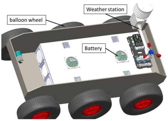
Figure 1.
The terrestrial 6 × 6 robot developed for identifying, monitoring, and intervening in risky areas. The structural elements of the robot include the command-and-control system, the battery system, and the weather station.
The literature suggests that a robot has artificial intelligence if the following hold:
- Its perception is constituted from a system of sensors, controllers, and software modules that are essential for moving from point A to point B. The perception system detects, classifies, and localizes natural and artificial features of the unstructured environment in which it moves. The specific objectives of the perception system for crossing a path, following a planned path and avoiding the obstacles, come from the necessary velocity of the vehicle and from the characteristics of the presumed working environment (the density of the obstacles, visibility, illumination, weather, and the edges of the road) so that the UGV can determine the corresponding velocity, stop, or avoid obstacles [4,17].
- When planning the paths that will be followed, a path is generated with no collisions in an environment with obstacles, and the path is optimized by respecting some criteria. This deals with the planning methods of global and local paths. The planning methods use the data captured by the sensors to estimate the parameters of the environment and moving the robot in real-time. The global method needs a completely known environment and certain simplifying methods; for the local method, the algorithm allows some real-time adjustments to the path to be followed. Planning implies optimization procedures of the time (and velocities) to select the geometrical paths in real-time to avoid obstacles [18,19,20,21]. Since every obstacle creates a risk level for the UGV, introducing proportional integrative derivative (PID) controllers and fuzzy logic methods, which classify the objects around the vehicle based on their level of risk, allows generating some predictions regarding the capacity to avoid fixed or moving obstacles (the velocity obstacle (VO) approach), which means that, virtually, a space that defines the respective object should be generated [22,23,24].
- The mission of a UGV agrees with path planning through adopting some algorithms that can generate optimal behavior and, each time discrepancies from the initial map appear, these data are updated. Thus, the error and cost functions increase the efficiency when crossing a certain space, and the search would become faster [25,26].
- The wireless communication and tele-command of a UGV with a ground control station (GCS) with an operator or with another robot are achieved through wireless mesh networks (WMNs). These networks are self-organized and dynamically auto-configured. For quality communication, these systems have scalability and security as objectives [27,28]. Tele-command is very important [28], even though its functionalities are due to its sensors; the video Infra-Red/Electro-Optical (IR/EO) devices and any other attached devices allow the sampling of data [29,30,31].
- The navigation system of a robot is a non-structured environment that uses path planning, obstacle avoidance and circumnavigating, localization, and perceptive interpretation techniques. All these cannot be combined in a single system (a single software application), which is why for each robotic system, a custom project must be realized with a software system that should be adapted to the respective application. A navigation architecture becomes efficient if the mobility of the robot is divided into specialized software modules. This architecture consists of software modularity (as a consequence of introducing a new sensor or maintaining some obstacle avoidance modules based on certain cinematics), robot location control based on the different functionalities and learning algorithms, techniques of time-domain analysis (response time of the sensors, temporal depth, space localization, and decision making based of the dynamics of the robot), and decoupled control [32,33,34,35,36].
- Implementing machine learning and deep learning techniques requires precise information so that the path planning allows locating the robot in space and memorizing the position of obstacles. UGVs are complex autonomous systems that use artificial intelligence (AI) through image recognition, human-machine interaction, intelligent decisions, logic, and learning. The deep learning algorithms restricted Boltzmann machines (RBMs), and convoluted neural networks (CNNs) are specially used for computer vision (CV) applications for object recognition. The data quantity necessitates using algorithms of the back-propagation types to compute the gradients and stochastic gradient descent optimization methods to minimize the errors in the outputs from the network as a function of the corresponding inputs. Apart from these, various auto-encoders, capsule networks, and synthetic gradients are needed, which we will discuss in future research in the domain of UGVs [37,38,39,40,41,42].
- Obstacles are defined as the elements that appear on the robot’s path—bumps and ditches are just elements of the road that are described in the equations of the contact of the engine with the ground.
The research part on autonomous movement (machine learning, deep learning, etc.) is already underway. The reviewers’ suggestions in this regard will be considered. For route planning, we think it is much better to focus on route planning algorithms such as Rapidly-Exploring Random Tree (RRT), Lattice, and the A* search algorithm.
2.2. The Controller
The implemented controllers integrate the systems, and the data flow was commercial off-the-shelf (COTS) accessible [43,44].
Figure 2 presents the three types of remote-control systems for terrestrial robots, which are currently described in the literature as follows:
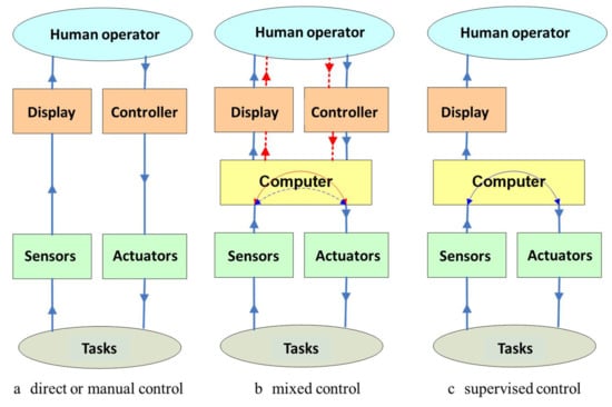
Figure 2.
Schematic representation of the three major classes of command-and-control systems of terrestrial robots. For ongoing research, on the use of 6 × 6 terrestrial robots for the purpose of identification, monitoring and intervention in risk areas, we proposed that of the three versions: (a) direct or manual control; (b) mixed control; (c) supervised control, to use version (b).
- Direct or manual control: The robot does not have artificial intelligence or autonomy, and the operator controls the movement of the robot directly without automatic aid; the principle of operation is very simple and is based on four bits (forward-backward and left-right), in which case signal identification is a priority, as the microcontroller timer is used as an internal counter so that it can calculate the pulse width from the motor shaft [45].
- Mixed control: The robot has a certain degree of artificial intelligence and/or autonomy, and the operator helps it to perform certain operations; to switch to autonomous mode, the system of sensors for orientation (gyroscope) and measurement of distances (odometer) make predictions about the next path to follow. The greater the distance from the operator, the more difficult the teleoperation, especially due to the visual effect on the operator due to the movements of the vehicle and the orientation of the camera. If the orientation of the camera does not correctly compensate for the vehicle’s rotation, it will cause a shunt of the camera and wrong decisions related to the movement of the vehicle [46].
- Supervised control: The robot has a high degree of intelligence and/or autonomy, while the user only intervenes at a high decision level. Control architectures are designed to allow the use of a single control law for each context: the route to the target, the avoidance of obstacles, etc. To manage the interactions between controllers depending on the context, multi-agent systems are used, which can self-organize depending on the emergence of phenomena [47].
The control architecture for the intervention robot was specific for autonomous navigation and is based on the Raspberry Pi 4, B/4 GB model controllers (for commanding the motors) (Distrelec GmbH Dresdnerstrasse 471200 Wien Austria), NVIDIA® Jetson Nano™ Developer Kit (video image processing) (Distrelec GmbH Dresdnerstrasse 471200 Wien Austria), and Pixhawk Autopilot (navigation) as shown in (Figure 3).
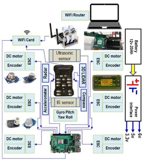
Figure 3.
The control and command architecture of the studied robot including obstacle detection (ultrasonic and infrared (IR) sensors); orientation (tri-axial accelerometer and global positioning system (GPS)), gyroscope (pitch, yaw, and roll), compass; DC motor encoder, Electronic Speed Controller (ESC); Pixhawk controller, Raspberry Pi 4 controller and NVIDIA Jetson Nano; power system, and Wi-Fi communication system.
This architecture (Figure 3) was designed to manage the interactions between the elementary controllers. The control laws allow reaching static or moving targets. Regarding the technical detail, the command-and-control system was structured in seven modules:
- i.
- The obstacle detection module, consisting mainly of sensors for measuring distance. The use of several types of sensors (ultrasonic, IR, and 3DLIDAR) was used to allow obtaining values as close as possible to reality. Each type of sensor had its own characteristics regarding the maximum/minimum measuring distance. The 3DLIDAR sensor had the role of performing an overall scan, allowing the lifting of a 3D survey of the area of interest. Overlapping information from the three types of sensors would provide a map of the terrain, including beyond the open view.
- ii.
- The orientation module, composed of inertial sensors, GPS, compass, magnetometer, gyroscope, was used to analyze the position of the robot but also the obstacles to the global and local reference system. This information passed through the displacement algorithm determining the optimal path between the local reference point and the final position. The final position could be variable or fixed. We are talking about fixed targets when we are dealing with stable emergencies. In general, the kinematic and dynamic characteristics of the targets can be variable. For example, the flames of a fire can have different intensities depending on the nature of the combustible material, the direction and speed of the wind, etc.
- iii.
- The motor supply voltage control module consisted of the encoder, and the electronic speed controller (ESC) has the role of modifying the speed and direction of rotation of the motors so that the robot can move on a certain route. It also knows when and how much energy to deliver to the engines when leaving the place or climbing some slopes or climbing some obstacles. In the case of intervention in terrorist actions (artisanal bombs, etc.), the engines must be very stable so that no vibrational phenomena occur. In addition to the traction motors, there will also be motors for the manipulator on the robot.
- iv.
- The module consisted of two types of controllers, Raspberry Pi and Pixhawk, which handled the management of all components of the robot. The Raspberry controller controlled the engines, managed the sensors, the power supply system. The Pixhawk controller handled the management of the navigation system.
- v.
- The module consists of an NVIDIA Jetson nano-controller; two video cameras had the mission of taking video images, analyzing them, and/or sending them wirelessly to the GCS in order to prepare the route to be followed by the robot. The Jeston nano-controller also had a master role.
- vi.
- The power supply module was a structure made up of Li-Ion batteries type 18,650, 5000 mAh, 3.7 V.
- vii.
- Wireless communication module: router and a cheap and available ESP8266 Wi-Fi module with full TCP/IP capability and microcontroller capability. It could be used with any Pixhawk, Raspberry Pi, or Jetson nano-controller.
2.3. External Sensor System
The sensor system of the robot consisted of sensors for dangerous substance detection (CO2, CO, CH4, and H2), gamma radiation detection (mass spectrometer), environment conditions determination (meteorological station: humidity, temperature, and air current detection), anemometer, 3D scanning (3D LiDAR), and images (IR/EO video cameras) [48,49,50]. In addition, the intervention for neutralizing an incident with explosive systems involves applying, in all circumstances, some procedures that represent a particular means of action adopted from the specialized personnel in neutralizing/destroying explosive systems or any dangerous material. The intervention robots for missions involving neutralizing explosive devices would be controlled through a remote command or remote control.
Tele-command implies the existence of a barrier between the user and the operating environment in two locations: the operator location and the robot location. The control of the mobile robots, based on remote operation, needs a robust system with an intuitive, flexible, and efficient interface. In the most common situations, mobile robots are equipped with sensors and controllable modules, which provide a significant amount of data for the user [50].
2.4. Propulsion System
The propulsion system consisted of six motors with a JGA25-370 gearbox (6 V, 281 rpm) and six wheels with rims composed of plastic (240 mm diameter, 75 mm tire width, and 20 mm shaft diameter). Each wheel is independent, and the motors were independently driven by electronic stability control (ESC) so that each wheel could be controlled, as shown in Figure 4.
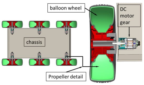
Figure 4.
Schematic representation of the propulsion system of the 6 × 6 robot for emergency situations consists of six motors with a gearbox, six wheels with rubber tires, and a nodular balloon inflated with air for more efficient damping of the unevenness of the route during movement of the robot.
The propulsion solution presented was made in the laboratory. In the future, we propose, together with a potential investor, to replace the wheeled propulsion system with a tracked one, thus reducing the size and gaining space for other components (payload). Replacing the wheeled train with a tracked one would also benefit from the progression in loose terrain or even crossing areas that are full of rubble. The aspect facilitates presented above executing the turns with minimal effort because the propulsion system has only two mobile wheels. The lack of a direction system leads to consistent friction with the ground.
3. Analytical Model
The studied robot was a multi-body system (MBS) [51,52] in which the components were categorized as rigid bodies. Researchers [52,53,54] have explained that a multi-body system is a finite set of rigid physically and geometrically interconnected bodies that are also connected to terrain that does not belong to the MBS. The MBS ensemble was built by establishing and imposing some kinematic and dynamic constraints that describe the interconnecting geometrical modes: freedom of degrees, forces, and torque.
To analyze a rigid body in a fixed coordinates system, the mathematical set of the position vectors of the complete structure and/or its components must be determined from a kinematics point of view. Since the environment in which the robot operates is an unstructured environment, the dynamics of the robot should consider the state of terrain, the type of terrain, its density, the loosening of the soil, humidity, etc. [53,54,55].
3.1. Kinematics of the Robot with a 6 × 6 Propulsion System
The kinematic model of the robot with six mobile wheels, without any of them being driving wheels, was generated based on some simplifying hypotheses [56,57]. The delay differential equations (DDEs) that describe the initial dimensional structure and use fewer parameters and state variables than the ordinary differential equation (ODE) and partial differential equation (PDE) systems are described in [16].
The robot was characterized by non-holonomic behavior because of the effects that appeared at the interaction of the wheels with the rolling path. According to this approach, the equations that describe the direction were differential equations so that the robot had high maneuverability, as shown in Figure 5. In fact, the kinematics diagram was specific to a 6 × 6 vehicle, for which an analytical-experimental model was developed [52,58,59,60]. The viability of the model was verified using a precise laser scanner for localizing the mobile robot in the conditions of the simplified hypotheses [61].
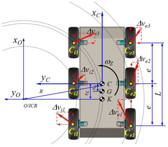
Figure 5.
The 6 × 6 kinematic diagrams of the robot showing the following essential characteristics for a simple and fast analysis of the robot kinematics: the six driving wheels are not steering wheels; turns are made by changing the rotational speeds of the six wheels; cornering radii varied depending on the rotational speed of the drive wheels and the indices of adhesion to the ground, the slip indices. If the movement was rectilinear, the decomposition of the speed was uniform only for the ideal conditions of movement; the ground contact of the balloon of the wheels was related to the pressure in the balloon. The weight of the robot and the position of the center of gravity may be altered, in particular, by the operating platforms.
Instantaneous center of rotation (ICR) values are dependent on the dynamics of the robot, which considers the slip ratio, but in an area with medium velocities, once the velocity increases, those values increase too.
For a robot with six mobile wheels, the velocities of the wheels are written as and the following convention . The calculus method of the direct kinematics in the plane can be defined as
where is the translational velocity of the robot, is the angular rate, and is the radius of the mobile wheels.
The instantaneous rotation centers are: ICR, ICRi, ICRe, and ICRCG; ICRi and ICRCG are on a line parallel to the OX axis a line parallel to the OX axis of the Cartesian coordinate system, thus determining the corresponding x and y coordinates:
The matrix is dependent on the ICR coordinates:
3.2. Dynamics of the Robot with a 6 × 6 Propulsion System
The study of the 6 × 6 dynamics was performed starting from the equations that describe its kinematics [58]. The analytical model shown in Figure 6 describes the movement based on the angular rate of the wheels. This algorithm was chosen because the velocity of the robot is given by the angular rate of the wheels, which were commanded by a controller by varying the input voltage. The dynamics of a robot terrestrial vehicle with six mobile wheels (non-driving) had two calculus models: 2D and 3D. Figure 6 depicts a diagram of the movement on 2D terrain.
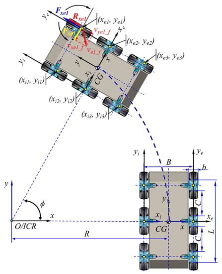
Figure 6.
Schematic of the 2D dynamics of the 6 × 6 robot, which had some specificities related to the choice of travel mode. The ground contact spots of the six wheels were identical. Working conditions are ideal when Md = Mr (Md—motor torque; Mr—resistant moment). The geometric center of the contact spots (yellow dots) during the turn is represented outside the geometric center of the contact spots. This representation suggests that progression in the field is influenced by different coefficients and that each operational platform can create an additional balance.
3.2.1. D Robotics Dynamics
The dynamic model of the robot is given by the following system of equations relating to the action of the forces upon the propulsion system:
where are the longitudinal slipping forces; are the lateral forces; are the drag forces; is the motor torque; is the resistant moment.
The tension (N/m2), or the unitary tangential effort in the wheel as a function of the deformation coefficient j, is given by
where (N/m2) is the normal pressure on the terrain, is the friction coefficient, and is the coefficient of the shear deformation module.
The longitudinal slip and lateral forces are
where is the movement of each wheel and is the angular velocity of the wheels.
3.2.2. D Robotics Dynamics
The dynamics of a terrestrial vehicle in an unstructured environment has a non-linear and varying characteristic in time. When the robot moves on tracks with slope α, its total weight can be separated into a component that is parallel to the rolling path (when it climbs a slope, its sign is negative as it opposes the movement of the robot; when it descends a slope, its sign is positive because the component becomes an active force) and a component perpendicular to the rolling path .
Figure 7 depicts the schematics of the drag at climbing the slope
where is the start drag, is the coefficient of influence of the masses in rotation, and refers to the total coefficient of friction
where is air drag, is the aerodynamic coefficient in standard aerodynamic conditions, is the air drag coefficient, and is the transversal surface of the robot.
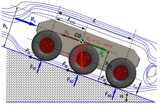
Figure 7.
A schematic of the 3D dynamics of the 6 × 6 robot showing the elements that influence the dynamic characteristics of a land vehicle: air resistance, friction force, robot weight, center of gravity position, wheel radius, and slope angle. The following figures will highlight other elements that contribute to influencing the law of motion of the robot.
Taking this perspective, Figure 8 depicts the schematics of climbing a step obstacle. Applying the Equations (11)–(14) regarding scaling an obstacle in steps, we obtained the friction coefficient corresponding to the step obstacle
where is the distance from the rear wheel shaft to the center of mass, measured on the direction of the imaginary line that passes through the center of the wheels; is the distance from the center of mass to the imaginary line that passes through the center of the wheels; is the radius of the wheels; is the height of the step obstacle; is the length of the imaginary line between the rear contact point and the edge of the obstacle (m); is the tilt angle of the shaft of the robot; is the friction coefficient corresponding to the step obstacle.
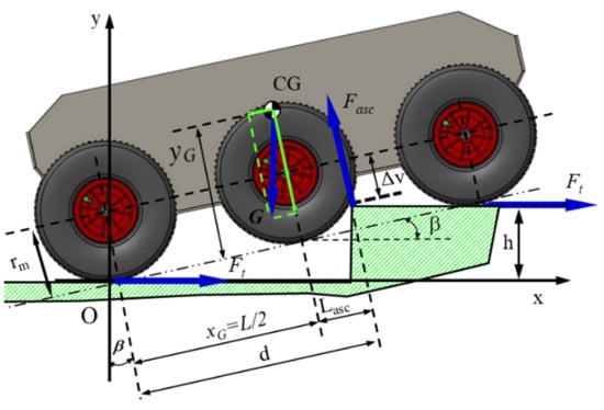
Figure 8.
Schematic of the escalation of a step-type obstacle by the robot. To ensure good ability to climb the step, the front, and middle wheels to be in permanent contact with the step to be climbed. It is not mandatory to have this situation; depending on the geometry of the workspace, energy consumption can increase, which affects the autonomy of movement. The robot was designed to move without being powered by a cable.
Following the application of Equations (11)–(14), it was possible to obtain the curves of variation in the angle of inclination of the towing platform through an analytical-numerical simulation, depending on the position of the center of gravity for the height (considered constant) of the step to be scaled, which is highlighted in Figure 9.
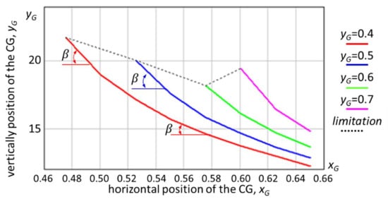
Figure 9.
The variation in as a function of the center of mass for h = 0.20 m (where h is the height of the step obstacle); the height of the step is constant. If the step to be scaled has a different height, the values in the graph will change. The pressure value of the wheel tires was not considered in this simulation.
Increasing the height of the ground robot’s center of gravity would allow it to tackle higher obstacles. However, obviously, for the accuracy of the calculation algorithm, the fact that the angle of approach of an obstacle increases means that the size of the drive wheel becomes important, and the distance between the axle of the front axle and the rear axle is also important. For example, there may be situations where a large wheelbase does not allow cornering, so the robot would not be prevented from completing the mission.
4. Simulation of the 6 × 6 Propulsion System
4.1. Simulation of Slope Climbing
To evaluate the potential to simulate the slope climbing, for longitudinal movement on a slope, the following must be considered: , the mass of the robot; , the thrust force; , the normal force; , the tilt angle of the longitudinal slope;, the distance between the center of mass and the shaft of the front deck; hcg, the distance between the center of mass and the rolling path surface (m); , the distance between the shafts; , the friction coefficient corresponding to the tilt angle of the slope (Figure 10); the moment for climbing the slope (Figure 11).
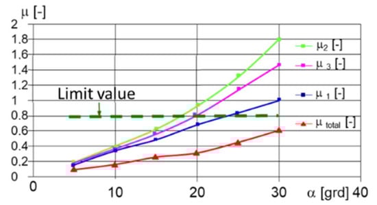
Figure 10.
The variation in the necessary for climbing a slope following the simulation using Equations (15)–(19). For the geometric characteristics of the robot and the total minimum adhesion coefficient, the robot could climb a step under the conditions of a CG (center of gravity of the robot) with a height = 0.20 m.
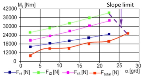
Figure 11.
The variation in the necessary as a function of the tilt angle of the slope.
The equations for the normal forces that act upon the wheels and for the minimum adhesion coefficient, which ensures using the thrust forces, are given in Equations (15)–(19):
The graphs in Figure 10 describe how the minimum coefficient of adhesion varies depending on the angle of inclination of the longitudinal slope. It can be easily observed that with the multiplication of the number of drive axles (two drive wheels for one axle), the grip capacity improved.
For the same geometric conditions and coefficients of friction with the ground (respectively, with the climb), Figure 11 displays the variation in the moment for climbing the slope.
4.2. Simulation of Crossing a Step-Type Obstacle
Crossing a step-type obstacle was simulated in two variants (Appendix A and Table A1):
- The obstacle was approached with both front deck wheels (Figure 12)
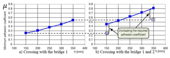 Figure 12. The variation in the necessary to cross an obstacle as a function of its height. The data used for the calculations are found in Appendix A and Table A1. Given the geometric characteristics of the towing robot and the mobile platform, and that changes are possible depending on the dimensions of the operational platforms, the robot can be used for different missions; we consider the data used to be sufficient: (a) crossing with bridge 1; (b) crossing with bridges 1 and 2.
 - The obstacle was approached with four wheels corresponding to the 1 and 2 decks (Figure 13)
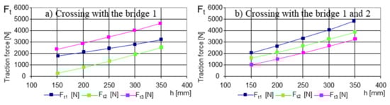 Figure 13. The variation in the necessary for crossing an obstacle as a function of its height. The explanations presented in Figure 12 also apply here: (a) crossing with bridge 1; (b) crossing with bridges 1 and 2.
Although, apparently, the index of the value of the minimum coefficient of adhesion provides information on the ability of a land vehicle to move, i.e., to be able to cling to the ground for progression, the graphs in Figure 12 provides precious information about when the robot has to climb an obstacle. In other words, the difference between the graphs in Figure 12a,b is obvious; with a safe drive axle (two-wheel drive), the climbing capacity was much lower, and energy consumption was increased.
With the escalation of an obstacle, the driving wheels would be in contact with it, successively (from the point of view of the obvious cinematic). But we could observe the distribution of the traction force on each drive axle (two conjugate drive wheels) Figure 13a. When the motor and the second axle came into contact with the obstacle, there was a new distribution of the traction forces, see Figure 13b. The new values of the traction forces showed that with the unloading of the weight force on another drive axle, the third axle required less pushing.
5. Testing the Braking When Descending a Slope in Dynamic Mode
The geometrical characteristics of the propulsion system, as the position of the center of mass of the mobile robot, are critical for ensuring stability in a static regime (Figure 14).
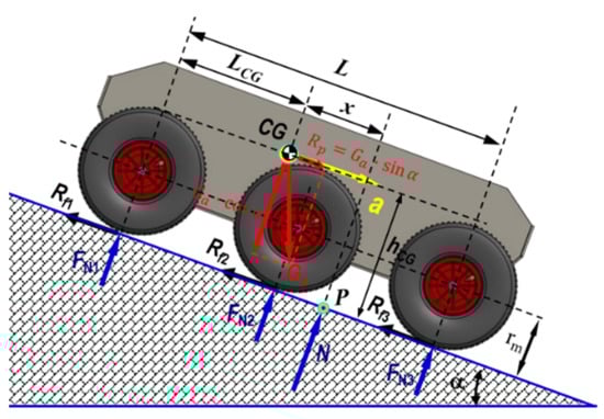
Figure 14.
Schematic of braking while descending a longitudinal slope. The dynamics of the robot during braking are much more suggestive when the process is diagrammed during the descent of a slope. In this case, two other notions intervene: a, deceleration when braking; , friction force.
From the viewpoint of the stability of the platform, while moving on a longitudinal slope, as outlined in Figure 14, the most difficult situation occurred during braking while descending on a slope, where represents the deceleration and is the braking force.
As can be seen in Figure 15, At the limit, the misalignment of the pressure center on the terrain becomes equal to , where, after solving the equilibrium equation of the torques around the P point, the deceleration becomes:
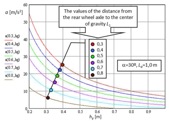
Figure 15.
The variation in the maximum deceleration at braking on a 30º slope as a function of the center of mass.
Thus, both increasing and moving it toward the front of the platform leads to decreasing the deceleration at braking because rollover could occur.
Robots with all the mobile wheels driven by electrical motors can brake by stopping the power supply or blocking the area of contact of the tire with the terrain; thus, at the limit, Equation (20) becomes:
After observing the measurements acquired by the accelerometers, we estimated that the analytical-numerical model would allow us to use it for the software necessary for autonomous navigation.
For clarity, the position of the body at a given time can be determined by integrating the accelerations measured in three mutually perpendicular directions and the angular velocities of rotation around the same axes (Figure 16).
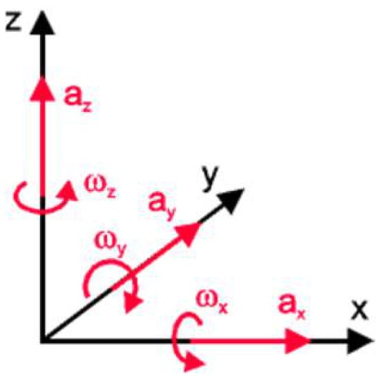
Figure 16.
Basic reference system for inertial navigation.
In Figure 17, the dynamic characteristics of the 6 × 6 robot when braking on the slope are determined with the help of an inertial sensor system.
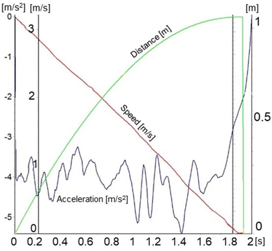
Figure 17.
The dynamic characteristics of the 6 × 6 robot when braking on the slope, determined with the help of an inertial sensor system.
The absolute speed measurement system based on inertial navigation was adopted because it allows the determination of the absolute speed of the robot. By integrating the data on accelerations and angular velocities, we determined the trajectory of the center of gravity.
The main limitation of this type of absolute speed measurement is the sensitivity and accuracy of the sensors used to measure accelerations and angular velocities. As high-precision sensors are expensive and require sophisticated calibration programs, a cheap calibration solution for the digital inertial sensor was adopted. We also considered the average of the vertical acceleration (along the z-axis) as equal to the gravitational acceleration. A GPS sensor was also used to increase the accuracy of the results. For this, the calibration solution consisted of applying the corrections for moving in three-dimensional space using the representation based on Euler’s angles and Euler’s rotation theorem, as can be seen in Figure 18.
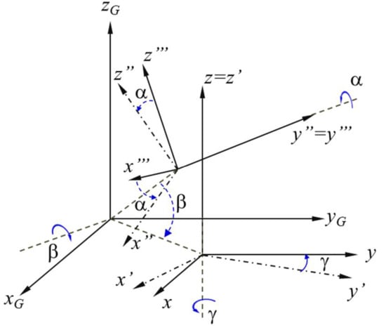
Figure 18.
Representation of the displacement of the coordinate system with the help of Euler’s angles.
In Figure 19, the longitudinal acceleration was determined using the derivative of the velocity, followed by filtering the resulted signal.
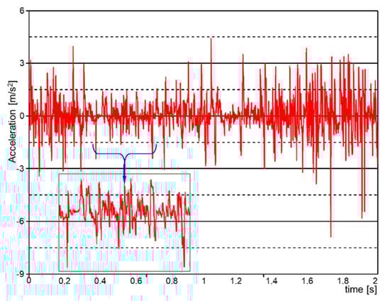
Figure 19.
The evolution of the longitudinal acceleration while braking on a slope, determined with the help of a GPS sensor system.
The importance of determining or measuring the acceleration during the braking of a vehicle is given primarily by the fact that we can determine the braking space. On the other hand, if the robot’s operating platform is equipped with, for example, a manipulator arm, the deceleration value helps us to determine how long the elements of the arm can be and what payload it can develop under certain travel conditions. Also, when using the robot to move dangerous substances or even an artisanal bomb equipped with vibration sensors, we must know the instantaneous variations of deceleration and acceleration.
6. Discussion of Potential Emergency Response Missions
The platform/carrier vector is the robot chassis, which was equipped with the propulsion, the command-and-control, and power supply systems. The platform/operational vector is a structure that can be interchangeable. Depending on the missions to be performed, the carrier vector can receive an operational vector. Next, we present two of the equipment possibilities for emergency interventions that we studied.
6.1. Emergency Response to Fires
The emergency response to fires requires an operational vector that can perform measurements on environmental conditions, the temperature of the affected area, and the types of harmful substances and their concentrations. Figure 20 depicts the elements that comprised a fire extinguishing system, which was moved to the risk area using a wheeled robot.
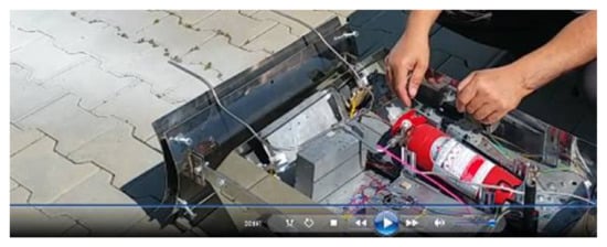
Figure 20.
Fire extinguishing system with two fire extinguishers and mechanism for maintaining the pressure of the extinguishing-type powder (Florex, E.12, Carbo, based on KHCO3).
After testing the fire extinguishing system, using a fire set with a cloth soaked in diesel, we examined the capacity of the robot to intervene in this scenario, so we list in Figure 21.
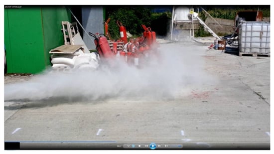
Figure 21.
Extinguishing jet performance. The fire was maintained by a pile of cotton cloths soaked in liquid fuel or diesel. When the smoke became sufficient and the wind direction changed toward the robot, the smoke sensors triggered the fire extinguishing system. The system was constructed with the help of two inert gas fire extinguishers.
Another aspect regarding the safety of the robot and the equipment of the robotic system is a flame protection shield, which was equipped to allow the robot to approach as close as possible to the fire. To highlight the characteristics of the elements that can influence the distribution and intensity of a fire, Figure 22 shows the data recorded with an Arduino-controlled weather station.
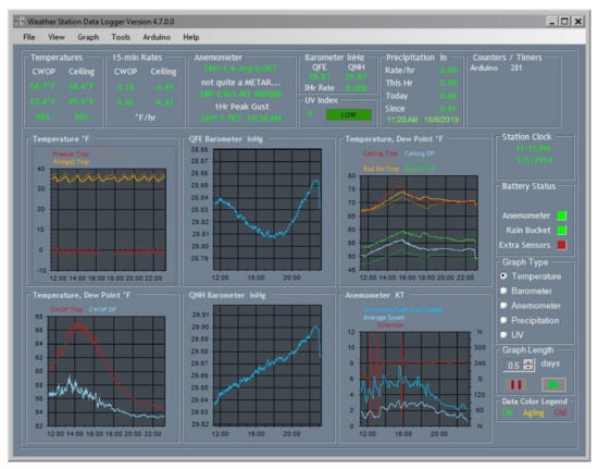
Figure 22.
Environmental samples taken with an Arduino-controlled weather station p/n 80,422. The values recorded by the weather station correspond to a summer period.
Figure 23 shows the simulation of the effects of high flame temperatures on the shield. As the purpose of this part of the study was to examine the effects of fire on the robot, we briefly present the concerns regarding the interventions that the robot could perform in emergency situations.
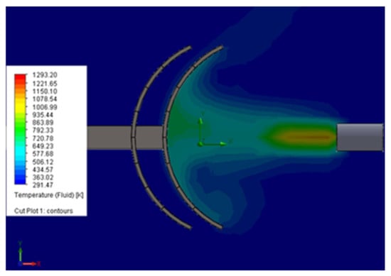
Figure 23.
Air temperature simulation for an output speed of 10 m/s. The numerical simulation was performed using the finite element simulation application Solid Works.
After testing the protection system with a stainless-steel shield, as shown in Figure 24, we verified the values obtained by numerical simulation.
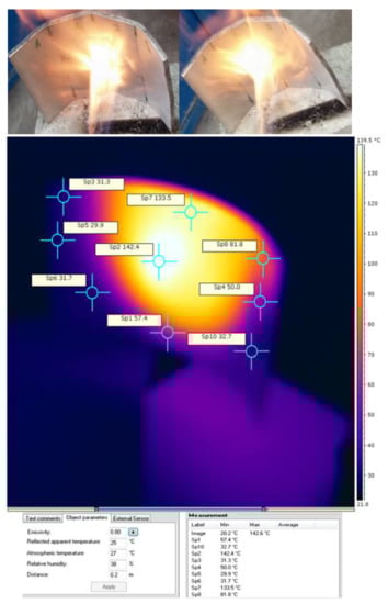
Figure 24.
Thermal study for target C (front view) direct contact with the flame at a temperature above 150 °C. Plate thickness: 4 mm, material: 316 L stainless steel, holding time: 4 min, and a concave shape.
6.2. Intervention in Emergencies Due to Gamma Radiation Emissions
An important issue during this experimental study was the use of modern solutions to ensure the transport of the measuring system through remote control systems such as robots. Some of the most important advantages of using a robotic system during a measurement operation in high-risk environments are the following:
- Improving safety by eliminating direct exposure of personnel to possible hazardous radiation.
- Reduction in operating time.
- The accuracy and precision of providing information.
- Reducing costs to help minimize the social and economic impact of possible accidents.
To minimize the risk of human exposure in hazardous environments, we aimed to perform an experiment consisting of transporting the detection equipment with a remote-controlled robot. Thus, the robot carried the equipment that was the subject of the first experiment on rough terrain to capture specific measurements to determine the radioactivity of the environment (Figure 25).
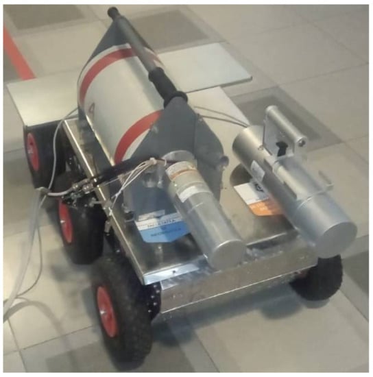
Figure 25.
Robotic system with an operational vector used to determine gamma radiation. The experiments were recorded at Titu Maiorescu University in Bucharest.
The data from Figure 26 are transmitted remotely via a secure connection from a laptop connected to the multichannel analyzer (MCA) and retrieved by specialized personnel to process it and make the necessary decisions.
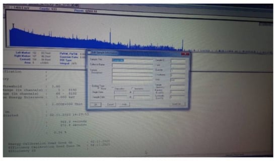
Figure 26.
Gamma radiation measurement with a Canberra dosimeter and spectrometer. The recorded values were part of the background of natural radiation. The values that stood out were specific to potassium. The purpose of data collection was to demonstrate the robot’s ability to perform different missions.
The representation in Figure 26 is a photo of data from the Canberra system, highlighting what can be measured with it.
7. Conclusions
Consistent with the results obtained, we found that our choice of geometric dimensions was appropriate as the values regarding the robot dynamics (Figure 10, Figure 11, Figure 12 and Figure 13), which were determined analytically, satisfy the mobility and stability requirements.
As the height of the center of mass increased, the characteristics when climbing stepping-type obstacles improved, but this advantage, above certain values (Figure 15), generated a loss of stability if the robot moved on a slope. This worsened under braking conditions when descending a slope (Figure 17).
Variations in acceleration and deceleration (Figure 17) lead to corresponding variations in traction forces and traction moments, which were identical to those that reflect the variation in acceleration. The variation in the traction forces, especially when turning, was influenced by the length of the adhesion surface because, with the increase in the width of the point of contact of the tire with the ground, the average pressure on the ground decreased, and the engine simultaneously sank, especially if the ground was deformable. Reducing the average pressure on the ground, even if it reduced the diving effect during a turn, also led to a reduction in the effect of lateral excavation. Another effect of reducing diving when the pressure on the ground decreased was that the grip decreased, so the wheel no longer gripped the ground very well. This side effect did not result in a significant reduction in traction (Figure 11). Overall (Figure 13), the total traction force was sufficient to move on soft ground and climb obstacles.
Inertial acceleration measurement systems are suitable for measuring decelerations/accelerations regardless of the type of rolling. The solution implemented with inertial sensors proves its effectiveness, especially when the robot is moving on rough terrain (specific to an unstructured environment). These results also reaffirm the idea that if the missions could be conducted in screened areas where satellite systems have no signal (caves, salt mines, subway, etc.), the inertial sensory system would allow the identification of specific parameters.
The processing of data captured by inertial sensors and using a GPS positioning system would be able to accurately determine the lateral sliding angle. The statement is based on the positioning error caused by the GCS (fixed station) being transmitted wirelessly to the robot so that the controller will be able to make the necessary corrections.
Author Contributions
Conceptualization, L.Ş.G.; O.A.; A.Ş.; D.G. and R.-I.B.; methodology, I.O.; software, C.M.; D.G., and D.C.; validation, A.Ş. and M.L.; formal analysis, D.C.; R.-I.B. and M.L.; investigation, O.A.; A.Ş. and C.M.; writing—original draft preparation, I.O. and L.Ş.G.; writing—review and editing, I.O. All authors have read and agreed to the published version of the manuscript.
Funding
This research received no external funding.
Institutional Review Board Statement
Not applicable.
Informed Consent Statement
Not applicable.
Data Availability Statement
Not applicable.
Acknowledgments
This study has benefited from material support and scientific consulting through the project with the following title: Demonstrator tehnologic—Robot de stins incendii (“Technological Demonstrator–Fire-Extinguishing robot”), with the identification Research Center of Excellence LUMINA (CEXLUM) contract number 587/09.09.2014. We thank the Research Center of the Faculty of Informatics of the “Titu Maiorescu” University, Bucharest, for the data from the Fire Extinguishing Robot—Fire Fighting Robot FFR-1 project. The robot participated in the first PatriotFest competition (https://www.patriotfest.ro/) in November 2017. The national PatriotFest competition was organized by the relevant Ministries of Defense, Home Affairs, Intelligence, and other subsidiaries in partnership with the New Strategy Centre Association.
Conflicts of Interest
The authors declare no conflict of interest.
Appendix A

Table A1.
The characteristics of the robot used for the simulation.
Table A1.
The characteristics of the robot used for the simulation.
| Radius of the wheels | 130.00 |
| Wheelbase | 400.00 |
| Distance between the front deck and the center of mass | 200.00 |
| Height of the center of mass related to the rolling path | 125.00 |
| Mass of the unequipped robot | 35.00 |
| Adhesion coefficient | 0.8 |
References
- Hoeppe, P. Trends in weather related disasters—Consequences for insurers and society. Weather Clim. Extrem. 2016, 11, 70–79. [Google Scholar] [CrossRef]
- Fire and Rescue Authorities Operational Guidance Generic Risk Assessment 3.10 Fighting Fires in Petrochemical Plant and Pipelines. Available online: https://assets.publishing.service.gov.uk/government/uploads/system/uploads/attachment_data/file/877073/GRA_3-10_archived.pdf (accessed on 24 February 2021).
- Nuță, I. Contributions to the Development and Improvement of Emergency Intervention Techniques. Ph.D. Thesis, Military Technical Academy “FERDINAND I”, Bucharest, Romania, 2013; p. 352. [Google Scholar]
- Virginia Tech Takes on Department of Defense Challenge to Build Disaster-Response Robots. Available online: https://vtnews.vt.edu/articles/2012/10/102412-engineering-thorrobotannouncement.html. (accessed on 24 February 2021).
- Kurvinen, K.; Smolander, P.; Pöllänen, R.; Kuukankorpi, S.; Kettunen, M.; Lyytinen, J. Design of a radiation surveillance unit for an unmanned aerial vehicle. J. Environ. Radioact. 2005, 81, 1–10. [Google Scholar] [CrossRef]
- Martínez, J.L.; Morales, J.; Sánchez, M.; Morán, M.; Reina, A.J.; Fernández-Lozano, J.J. Reactive Navigation on Natural Envi-ronments by Continuous Classification of Ground Traversability. Sensors 2020, 20, 6423. [Google Scholar] [CrossRef] [PubMed]
- Yukihisa, S.; Takeshi, S.; Yukiyasu, N.; Atsuya, K.; Tatsuo, T. The Aerial Radiation Monitoring in Japan after the Fukushima Daiichi Nuclear Power Plant Accident. Prog. Nucl. Sci. Technol. 2014, 4, 76–80. [Google Scholar]
- Lowdon, M.; Martin, P.G.; Hubbard, M.; Taggart, M.; Connor, D.T.; Verbelen, Y.; Sellin, P.; Scott, T.B. Evaluation of Scintillator Detection Materials for Application within Airborne Environmental Radiation Monitoring. Sensors 2019, 19, 3828. [Google Scholar] [CrossRef]
- Chee, F.T.; Sivakumar, D.M. Fire Fighting Mobile Robot: State of the Art and Recent Development, Malacca. Aust. J. Basic Appl. Sci. 2013, 7, 220–230. [Google Scholar]
- Grigore, L.Ș.; Soloi, A.; Tiron, O.; Răcuciu, C. Fundamentals of Autonomous Robot Classes with a System of Stabilization of the Gripping Mechanism. Adv. Mater. Res. 2013, 646, 164–170. [Google Scholar] [CrossRef]
- Park, J.-H.; Kim, B.-W.; Park, D.-J.; Kim, M.-J. A System Architecture of Wireless Communication for Fire-Fighting Robots. IFAC Proc. Vol. 2008, 41, 5303–5307. [Google Scholar] [CrossRef]
- Nuţă, I.; Orban, O.; Grigore, L. Development and Improvement of Technology in Emergency Response. Procedia Econ. Financ. 2015, 32, 603–609. [Google Scholar] [CrossRef]
- Grigore, L.S.; Priescu, I.; Joita, D.; Oncioiu, I. The Integration of Collaborative Robot Systems and Their Environmental Impacts. Processes 2020, 8, 494. [Google Scholar] [CrossRef]
- Gomez, J.C.; Ceballos, M.N.D. Hardware and software architecture for a Rover robot. Revista Avances en Sistemas e Informática Medellín 2011, 8, 494. [Google Scholar] [CrossRef]
- Anderson, J.; Lee, D.-J.; Schoenberger, R.; Wei, Z.; Archibald, J. Semi-autonomous unmanned ground vehicle control system. Def. Secur. Symp. 2006, 6230, 62301. [Google Scholar] [CrossRef]
- Grigore, L.Ș.; Priescu, I.; Grecu, D.L. Applied Artificial Intelligence in Fixed and Mobile Robotic Systems. Cap 4 Terrestrial Mobile Robots; AGIR: Bucharest, Romania, 2020; p. 703. ISBN 978-973-72-0767-8. [Google Scholar]
- Millard, F.R.; Aggarwal, R.; David, E.; Aspens, D.E.; Feddema, J.T.; Goodwine, J.W., Jr.; Kelly, C.W., III; Lehowicz, L.; McLaughlin, A.J.; Murphy, R.R.; et al. Technology Development for Army Unmanned Ground Vehicles; The National Academies Press: Washington, DC, USA, 2002. [Google Scholar]
- Wu, Q.; Chen, Z.; Wang, L.; Lin, H.; Jiang, Z.; Li, S.; Chen, D. Real-Time Dynamic Path Planning of Mobile Robots: A Novel Hybrid Heuristic Optimization Algorithm. Sensors 2019, 20, 188. [Google Scholar] [CrossRef]
- Kim, C.; Kim, Y.; Yi, H. Fuzzy Analytic Hierarchy Process-Based Mobile Robot Path Planning. Electronics 2020, 9, 290. [Google Scholar] [CrossRef]
- Hegedus, T.; Németh, B.; Gáspár, P. Design of a Low-complexity Graph-Based Motion-Planning Algorithm for Autonomous Vehicles. Appl. Sci. 2020, 10, 7716. [Google Scholar] [CrossRef]
- Guo, F.; Wang, S.; Yue, B.; Wang, J. A Deformable Configuration Planning Framework for a Parallel Wheel-Legged Robot Equipped with Lidar. Sensors 2020, 20, 5614. [Google Scholar] [CrossRef] [PubMed]
- Sun, J.; Liu, G.; Tian, G.; Zhang, J. Smart Obstacle Avoidance Using a Danger Index for a Dynamic Environment. Appl. Sci. 2019, 9, 1589. [Google Scholar] [CrossRef]
- Zuhaib, K.M.; Khan, A.M.; Iqbal, J.; Ali, M.A.; Usman, M.; Ali, A.; Yaqub, S.; Lee, J.Y.; Han, C. Collision Avoidance from Multiple Passive Agents with Partially Predictable Behavior. Appl. Sci. 2017, 7, 903. [Google Scholar] [CrossRef]
- Geng, X.; Wang, Y.; Wang, P.; Zhang, B. Motion Plan of Maritime Autonomous Surface Ships by Dynamic Programming for Collision Avoidance and Speed Optimization. Sensors 2019, 19, 434. [Google Scholar] [CrossRef] [PubMed]
- De Cos-Cholula, H.E.; Diaz-Arango, G.U.; Hernandez-Martinez, L.; Vazquez-Leal, H.; Sarmiento-Reyes, A.; Sanz-Pascual, M.T.; Herrera-May, A.L.; Castaneda-Sheissa, R. FPGA Implementation of Homotopic Path Planning Method with Automatic As-signment of Repulsion Parameter. Energies 2020, 13, 2623. [Google Scholar] [CrossRef]
- Gwon, J.; Kim, H.; Bae, H.; Lee, S. Path Planning of a Sweeping Robot Based on Path Estimation of a Curling Stone Using Sensor Fusion. Electronics 2020, 9, 457. [Google Scholar] [CrossRef]
- Akyildiz, I.; Wang, X. A survey on wireless mesh networks. IEEE Commun. Mag. 2005, 43, S23–S30. [Google Scholar] [CrossRef]
- Rao, N. Dynamic Data Transmission Using Wireless Sensor Networks. Int. J. Adv. Res. Comput. Sci. Softw. Eng. 2014, 4, 837–841. [Google Scholar]
- Parasuraman, R.; Caccamo, S.; Baberg, F.; Ogren, P.; Neerincx, M. A New UGV Teleoperation Interface for Improved Awareness of Network Connectivity and Physical Surroundings. J. Hum. Robot Interact. 2017, 6, 48. [Google Scholar] [CrossRef]
- Liu, S.; Atia, M.M.; Gao, Y.; Noureldin, A. Adaptive Covariance Estimation Method for LiDAR-Aided Multi-Sensor Integrated Navigation Systems. Micromachines 2015, 6, 196–215. [Google Scholar] [CrossRef]
- Grace, P.; Hughes, D.; Porter, B.; Alcock, P.; Coulson, G.; Blair, G. Middleware Support for Dynamic Reconfiguration in Sensor Networks. Available online: https://eprints.lancs.ac.uk/id/eprint/42464/2/grace09reconfiguration.pdf (accessed on 24 February 2021).
- Azouaoui, O.; Oudah, N.; Mansour, I.; Sema, A. Soft-computing based navigation approach for a bi-steerable mobile robot, Kybernetes. Int. J. Syst. Cybern. 2013, 42, 241–267. [Google Scholar] [CrossRef]
- Ravankar, A.; Ravankar, A.A.; Rawankar, A.; Hoshino, Y.; Kobayashi, Y. ITC: Infused Tangential Curves for Smooth 2D and 3D Navigation of Mobile Robots. Sensors 2019, 19, 4384. [Google Scholar] [CrossRef] [PubMed]
- Siegwart, R.; Nourbakhsh, I.R. Introduction to Autonomous Mobile Robots, a Bradford Book; The MIT Press: Cambridge, MA, USA, 2004; p. 335. ISBN 0-262-19502-X. [Google Scholar]
- Xiao, P.; Ju, H.; Li, Q.; Chen, F. Task Planning of Space-Robot Clusters Based on Modified Differential Evolution Algorithm. Appl. Sci. 2020, 10, 5000. [Google Scholar] [CrossRef]
- Pandey, A.; Parhi, D.R. New algorithm for behaviour-based mobile robot navigation in cluttered environment using neural network architecture. World J. Eng. 2016, 13, 129–141. [Google Scholar] [CrossRef]
- Yakub, F.; Abu, A.; Sarip, S.; Mori, Y. Study of Model Predictive Control for Path-Following Autonomous Ground Vehicle Control under Crosswind Effect. J. Control Sci. Eng. 2016, 2016, 1–18. [Google Scholar] [CrossRef]
- Gao, Y. Model Predictive Control for Autonomous and Semiautonomous Vehicles. Ph.D. Thesis, University of California, Berkeley, CA, USA, 2014.
- O’Mahony, N.; Campbell, S.; Krpalkova, L.; Riordan, D.; Walsh, J.; Murphy, A.; Ryan, C. Deep Learning for Visual Navigation of Unmanned Ground Vehicles: A review. In Proceedings of the 2018 29th Irish Signals and Systems Conference (ISSC), Belfast, UK, 21–22 June 2018; pp. 1–6. [Google Scholar]
- Shan, T. Minimalistic and Learning-Enabled Navigation Algorithms for Unmanned Ground Vehicles. Ph.D. Thesis, Faculty of the Stevens Institute of Technology, Hoboken, NJ, USA, 2019. [Google Scholar]
- Zhang, T.; Li, Q.; Zhang, C.-S.; Liang, H.-W.; Li, P.; Wang, T.-M.; Li, S.; Zhu, Y.-L.; Wu, C. Current trends in the development of intelligent unmanned autonomous systems. Front. Inf. Technol. Electron. Eng. 2017, 18, 68–85. [Google Scholar] [CrossRef]
- Toma, Ș.A.; Sebacher, B.; Focșa, A.; Pura, M.L. On Anomalous Deformation Profile Detection Through Supervised and Un-supervised Machine Learning. In Proceedings of the IGARSS 2019—2019 IEEE International Geoscience and Remote Sensing Symposium, Yokohama, Japan, 28 July–2 August 2019; pp. 7419–7422. [Google Scholar] [CrossRef]
- Appelqvist, P.; Knuuttila, J.; Ahtiaine, J. Mechatronics Design of an Unmanned Ground Vehicle for Military Applications. In Mechatronic Systems Applications; IntechOpen: London, UK, March 2010; Chapter 15; pp. 28–32. [Google Scholar] [CrossRef][Green Version]
- Al-Mayyahi, A.; Wang, W.; Hussein, A.A.; Birch, P. Motion control design for unmanned ground vehicle in dynamic environment using intelligent controller. Int. J. Intell. Comput. Cybern. 2017, 10, 530–548. [Google Scholar] [CrossRef]
- Saputra, H.M.; Mirdanies, M. Controlling unmanned ground vehicle via 4 channel remote control. Energy Procedia 2015, 68, 381–388. [Google Scholar] [CrossRef]
- Norberg, M.; Söderbäck, N.E. Design and Implementation of an Intuitive Control Method for Tracked UGVs. Master’s Thesis, KTH Industrial Engineering and Management, Stockholm, Sweden, 8 March 2011. [Google Scholar]
- Dafflon, B.; Vilca, J.; Gechter, F.; Adouane, L. Adaptive Autonomous Navigation using Reactive Multi-agent System for Control Law Merging. Procedia Comput. Sci. 2015, 51, 423–432. [Google Scholar] [CrossRef]
- Aleksandar, R.; Khalid, A.; Mirko, J. Sensor-Based Intelligent Navigation and Control of Autonomous Mobile Robots for Advanced Terrain Missions. Sci. Tech. Rev. 2010, 60, 7–15. [Google Scholar]
- Liu, G.; Zeng, W.; Feng, B.; Xu, F. DMS-SLAM: A General Visual SLAM System for Dynamic Scenes with Multiple Sensors. Sensors 2019, 19, 3714. [Google Scholar] [CrossRef] [PubMed]
- Lu, X.; Fei, J. Study of a MEMS Vibratory Gyroscope Using Adaptive Iterative Learning Control. Int. J. Adv. Robot. Syst. 2014, 11, 151. [Google Scholar] [CrossRef]
- Xu, Z.; Guo, S.; Song, T.; Zeng, L. Robust Localization of the Mobile Robot Driven by Lidar Measurement and Matching for Ongoing Scene. Appl. Sci. 2020, 10, 6152. [Google Scholar] [CrossRef]
- Wong, J.Y. Terramechanics and Off-Road Vehicle Engineering: Terrain Behaviour, Off-Road Vehicle Performance and Design, 2nd ed.; Butterworth-Heinemann: Oxford, UK, 2009; p. 488. ISBN 978-0-75-068561-0. [Google Scholar]
- Ciobotaru, T. Semi-Empiric Algorithm for Assessment of the Vehicle Mobility. Leonardo Electron. J. Pract. Technol. 2009, 8, 19–30. [Google Scholar]
- Alexa, O.; Coropețchi, I.; Vasile, A.; Oncioiu, I.; Grigore, L. Ștefăniță Considerations for Determining the Coefficient of Inertia Masses for a Tracked Vehicle. Sensors 2020, 20, 5587. [Google Scholar] [CrossRef]
- Pop, N.; Cioban, H.; Horvat-Marc, A. Finite element method used in contact problems with dry friction. Comput. Mater. Sci. 2011, 50, 1283–1285. [Google Scholar] [CrossRef]
- Wong, J.Y. Theory of Ground Vehicles, 3rd ed.; John Wiley & Sons Inc.: New York, NY, USA, 2001; p. 560. ISBN 13 978-0-471-35461-1. [Google Scholar]
- Dénes, T.; Gábor, S. Contact patch memory of tyres leading to lateral vibrations of four-wheeled vehicles. Philos. Trans. R. Soc. A Math. Phys. Eng. Sci. 2013, 371, 12. [Google Scholar]
- Wong, J.Y.; Chiang, C.F. A general theory for skid steering of tracked vehicles on firm ground. Proc. Inst. Mech. Eng. Part D J. Automob. Eng. 2001, 215, 343–355. [Google Scholar] [CrossRef]
- Yu, W.; Chuy, O.; Collins, E.G.; Hollis, P. Dynamic Modeling of a Skid-steered Wheeled Vehicle with Experimental Verification. In Proceedings of the 2009 IEEE/RSJ International Conference on Intelligent Robots and Systems, St Louis, MO, USA, 11–15 November 2009; pp. 4212–4219. [Google Scholar] [CrossRef]
- Cojocaru-Greblea, T.; Bontoș, D.; Vasiliu, N.; Dobre, A. Redundant Steering Systems for Articulated Vehicles. In Proceedings of the 17th International Multidisciplinary Scientific GeoConference SGEM 2017, Albena, Bulgaria, 29 June–5 July 2017. [Google Scholar] [CrossRef]
- Gao, J.; Ye, W.; Guo, J.; Li, Z. Deep Reinforcement Learning for Indoor Mobile Robot Path Planning. Sensors 2020, 20, 5493. [Google Scholar] [CrossRef] [PubMed]
Publisher’s Note: MDPI stays neutral with regard to jurisdictional claims in published maps and institutional affiliations. |
© 2021 by the authors. Licensee MDPI, Basel, Switzerland. This article is an open access article distributed under the terms and conditions of the Creative Commons Attribution (CC BY) license (http://creativecommons.org/licenses/by/4.0/).