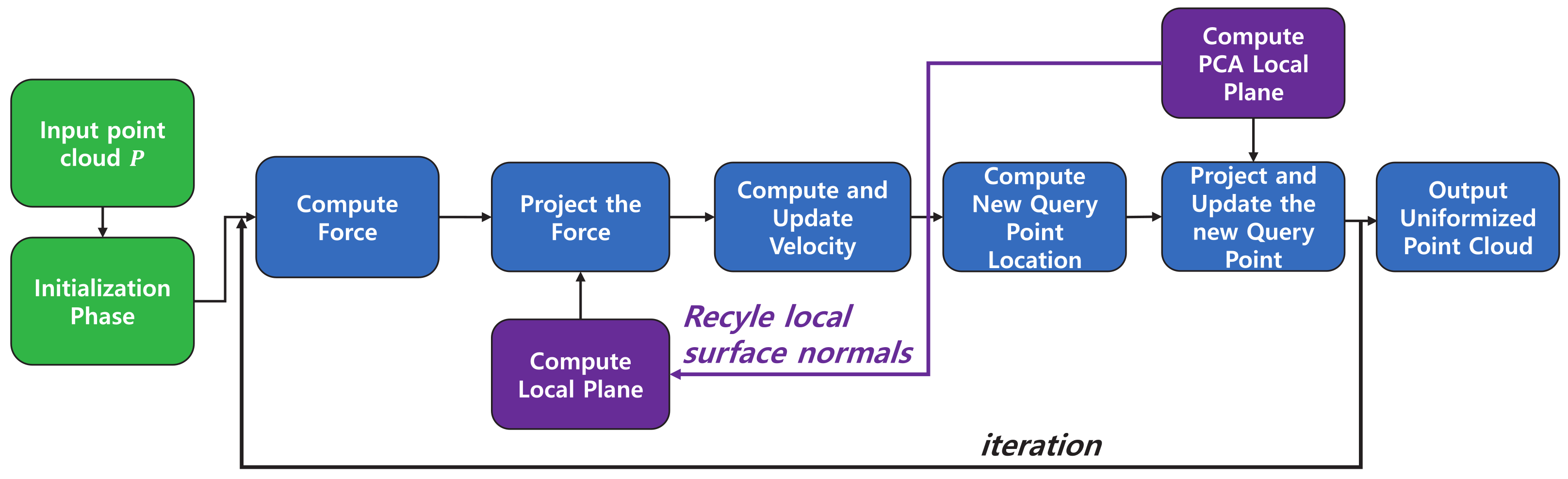
Figure 1.
Overview of point cloud resampling algorithm. The input point cloud P is assumed to be zero-centered and rescaled. First, the resampled point cloud , velocity , and the normal vectors of the local tangent plane are initialized. In each iteration, we perform the following procedures: We compute the K-nearest neighbors from to calculate the net electric force. Then, the normal vectors of the local tangent planes, calculated in the previous iteration, are used to project the forces to the local surfaces. The next velocities and the new query point cloud are computed based on the forces additionally modified with damping terms. Then, we obtain the K-nearest neighbor for the updated point cloud and calculate the local tangent planes. To prevent from diverging, we project it using these new tangent planes. These planes can be reused in the next iteration to project electric forces for efficiency. After the iteration converges, the final output point cloud is rescaled to the original scale and is relocated to have the original center point.
![Sensors 21 07768 g001]()
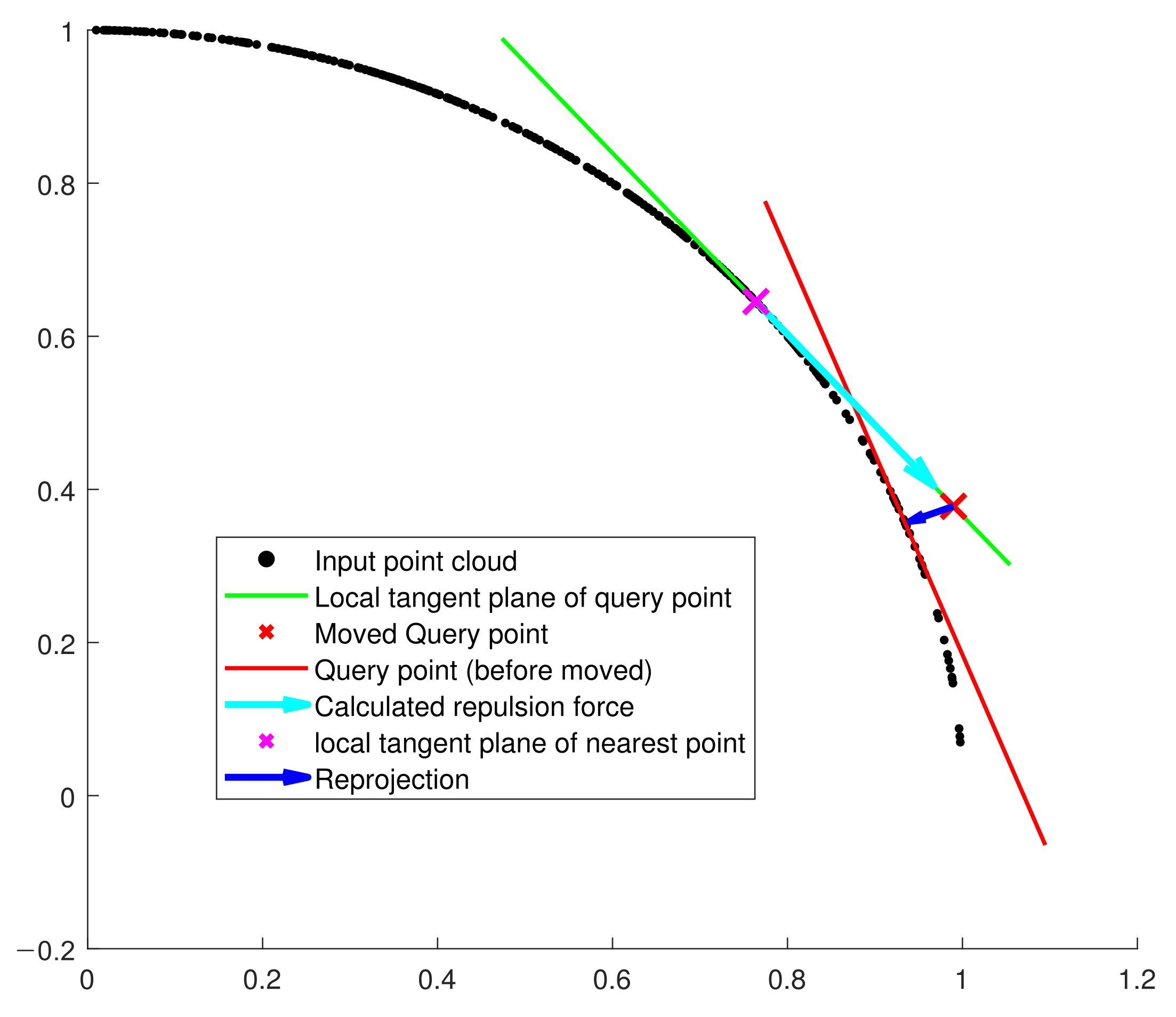
Figure 2.
PCA projection restrains the surface approximation error when moved points shift away from the input point cloud’s surface. By using the PCA projection, we project the moved points to the nearest local plane.
Figure 2.
PCA projection restrains the surface approximation error when moved points shift away from the input point cloud’s surface. By using the PCA projection, we project the moved points to the nearest local plane.
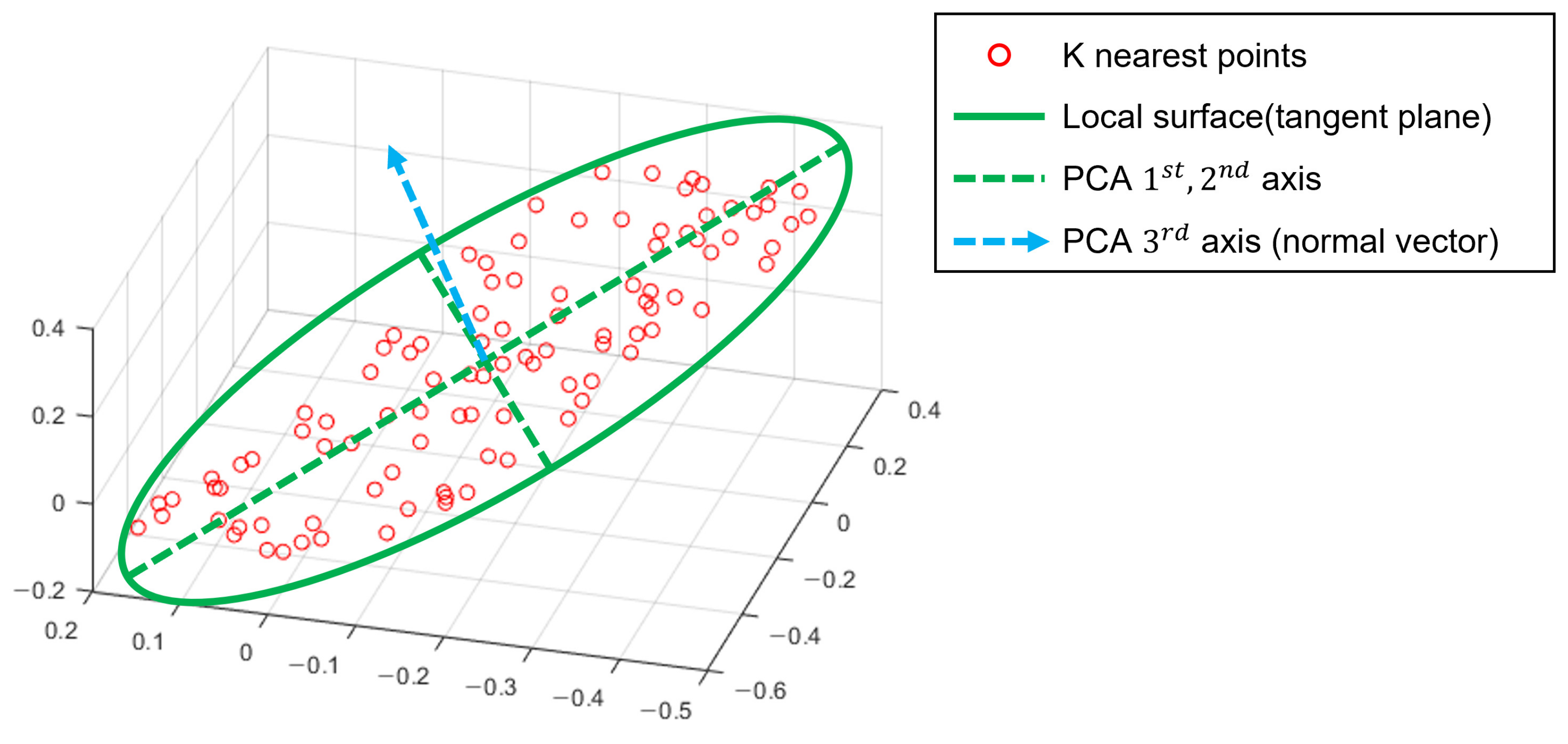
Figure 3.
Conceptual image of PCA-based local surface extraction. In a 3D space, the normal vector of the plane is the 3rd eigenvector of the PCA result.
Figure 3.
Conceptual image of PCA-based local surface extraction. In a 3D space, the normal vector of the plane is the 3rd eigenvector of the PCA result.
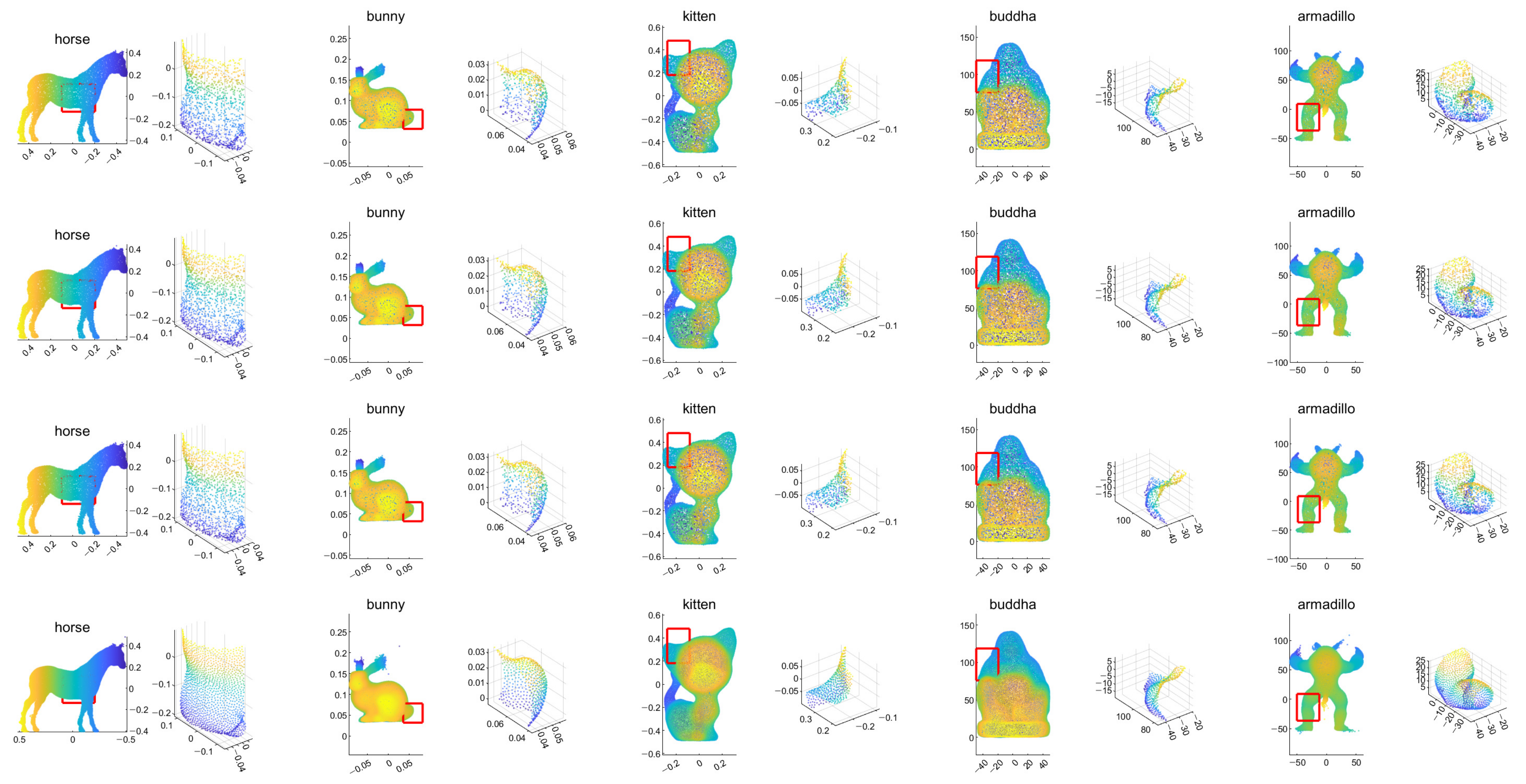
Figure 4.
Example results for the tangential noise cases. The first row is the input point cloud, the second row is the resampling result of the LOP algorithm, the third row is that of the WLOP, and the final row is that of the proposed algorithm. The odd columns are the resampled point cloud (from left to right, Horse, Bunny, Kitten, Buddha, and Armadillo), and the even columns are the corresponding enlarged views.
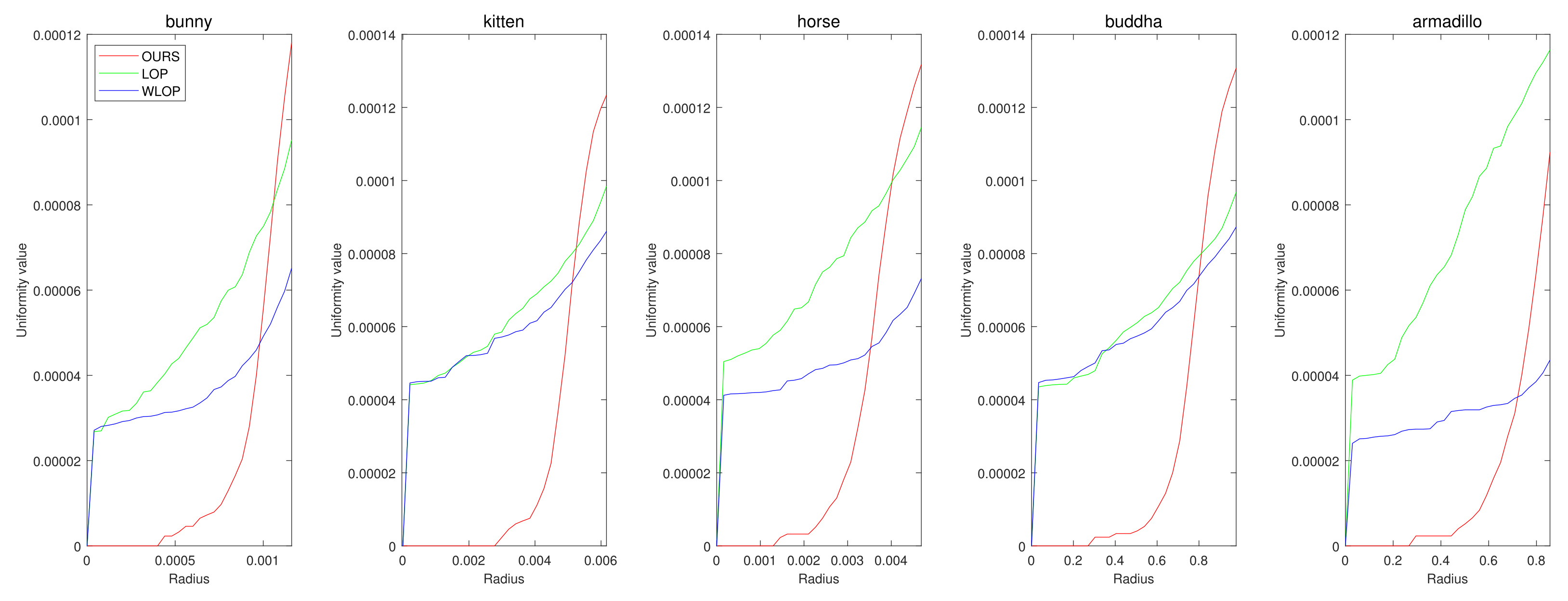
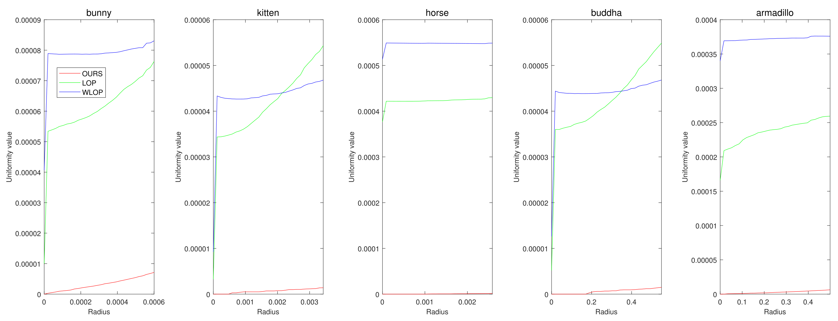
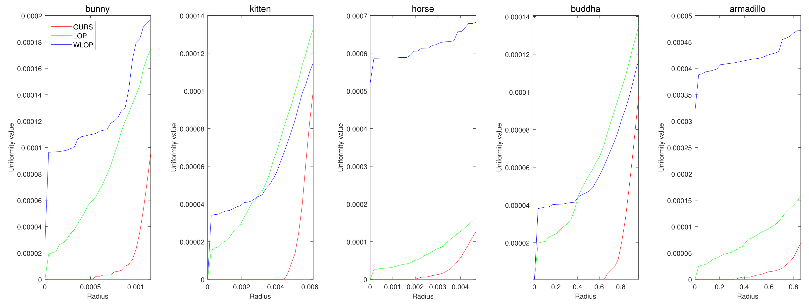
Figure 5.
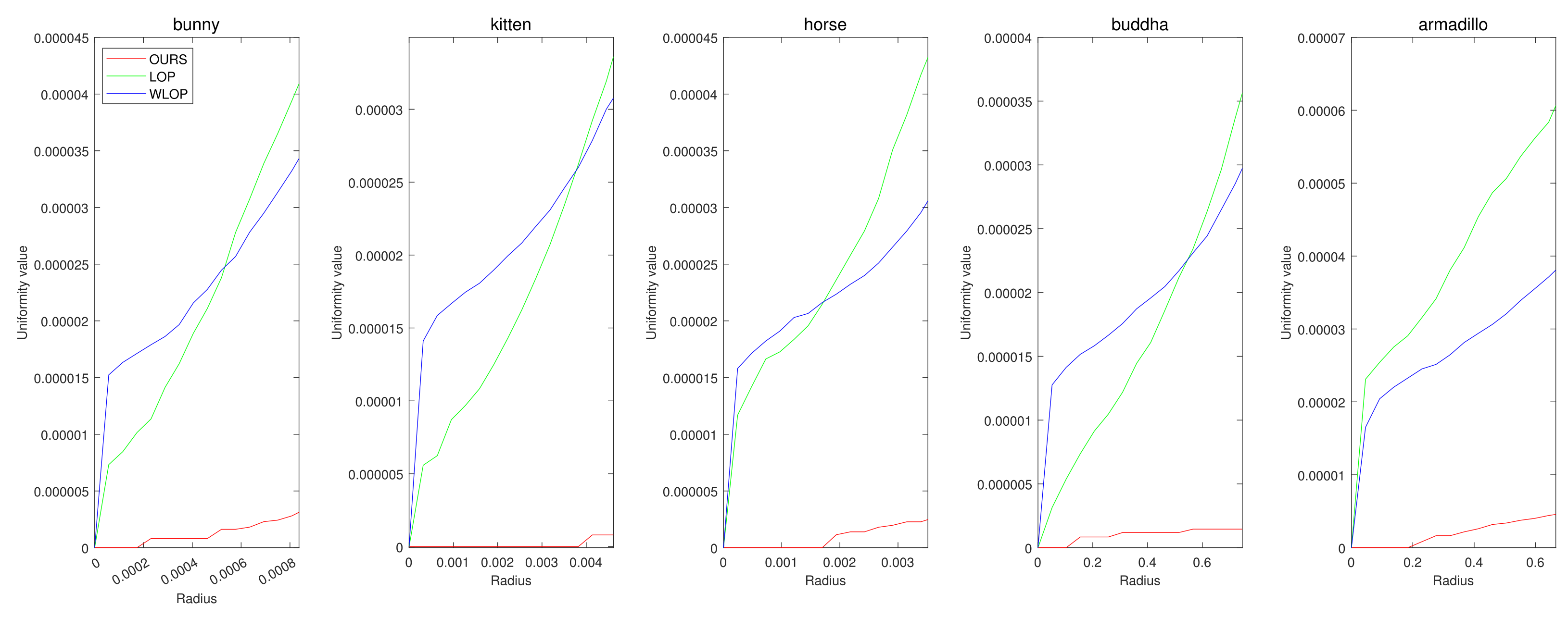
Quantitative results for the tangential noise cases. Each column shows the results of algorithms applied to Horse, Bunny, Kitten, Buddha, and Armadillo. The x-axes in the plots indicate the radius of evaluating u. The ranges of the radius were determined proportional to the square roots of the ratios between the surface areas of point clouds and the numbers of points.
Figure 5.
Quantitative results for the tangential noise cases. Each column shows the results of algorithms applied to Horse, Bunny, Kitten, Buddha, and Armadillo. The x-axes in the plots indicate the radius of evaluating u. The ranges of the radius were determined proportional to the square roots of the ratios between the surface areas of point clouds and the numbers of points.
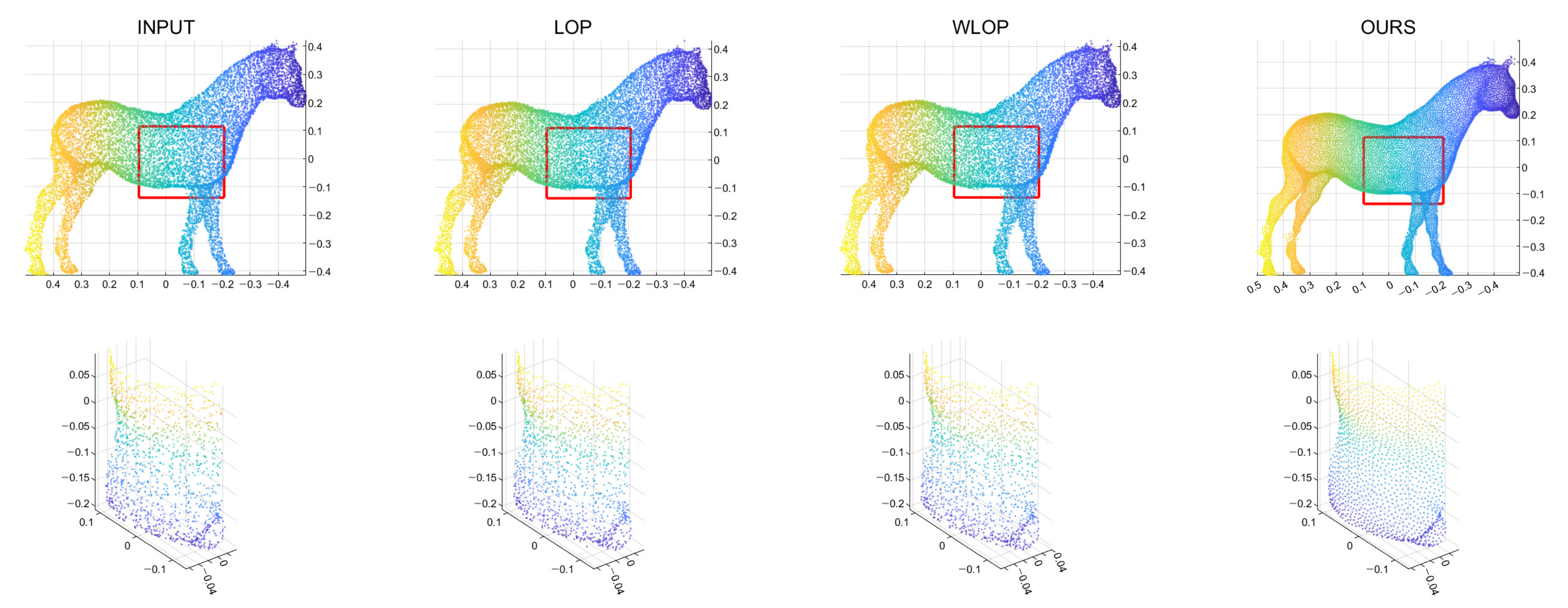
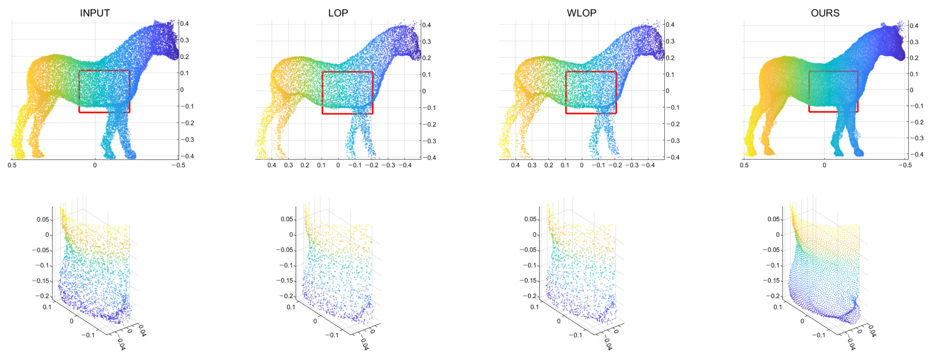
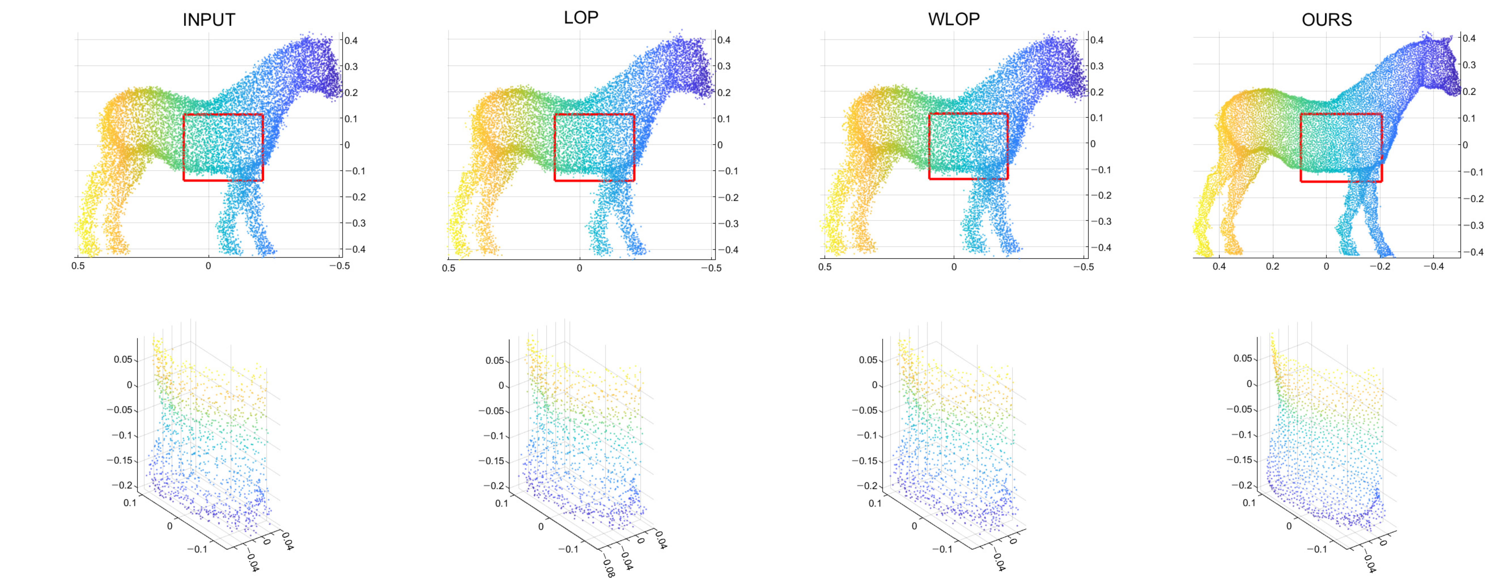
Figure 6.
Qualitative results for a tangential noise case (Horse). The second row shows the enlarged views of the red boxes in the first row. The first column shows the input point cloud. The second column shows the result of the LOP. The third column shows that of the WLOP. The last column shows that of the proposed algorithm.
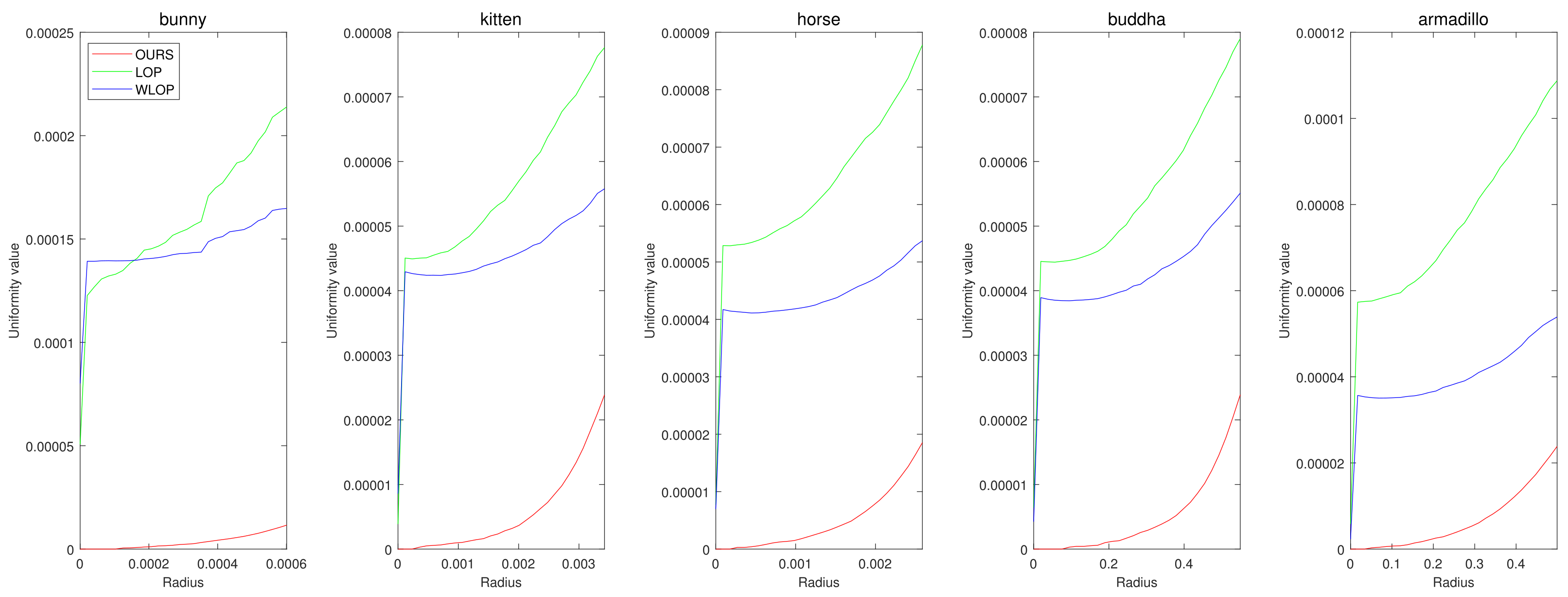
Figure 7.
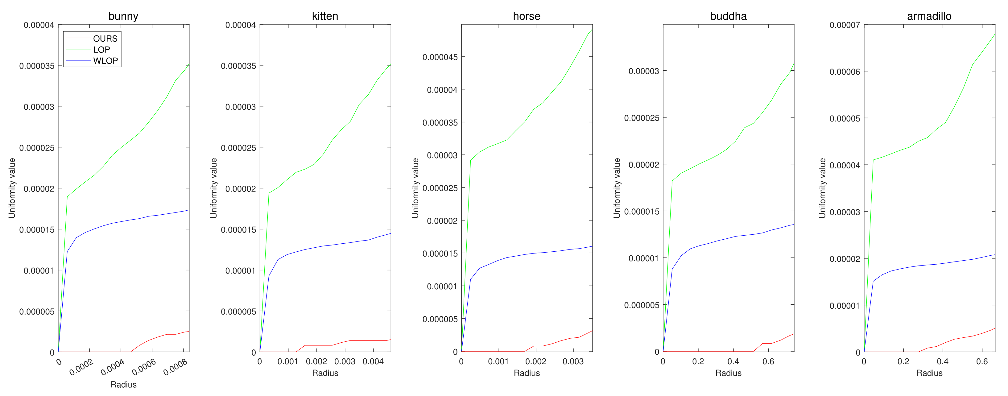
Quantitative results for the omnidirectional noise cases. Each column represents different input data (first column: Horse; second column: Bunny; third column: Kitten; fourth column: Buddha; and fifth column: Armadillo).
Figure 7.
Quantitative results for the omnidirectional noise cases. Each column represents different input data (first column: Horse; second column: Bunny; third column: Kitten; fourth column: Buddha; and fifth column: Armadillo).
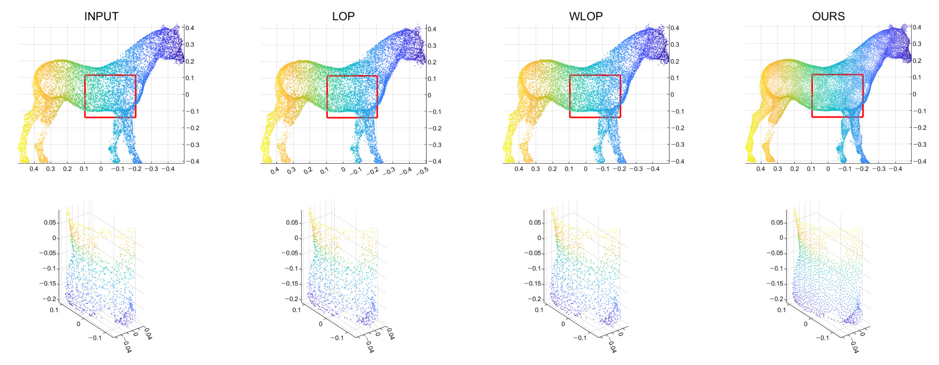
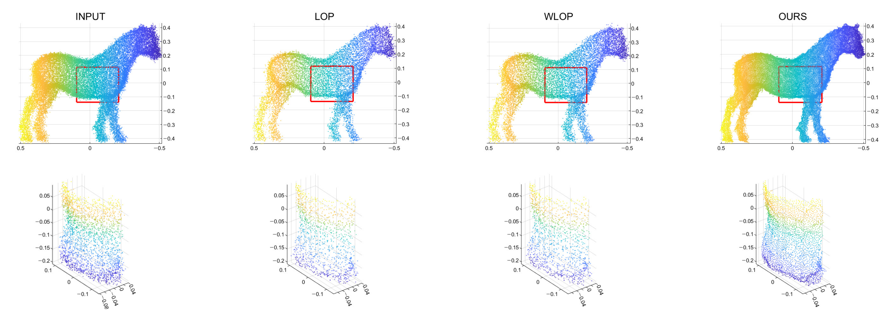
Figure 8.
Qualitative results for an omnidirectional noise case (Horse). First column: input point cloud; second column: LOP; third column: WLOP; and fourth column: proposed method. The second row shows enlarged views of the first row.
Figure 8.
Qualitative results for an omnidirectional noise case (Horse). First column: input point cloud; second column: LOP; third column: WLOP; and fourth column: proposed method. The second row shows enlarged views of the first row.
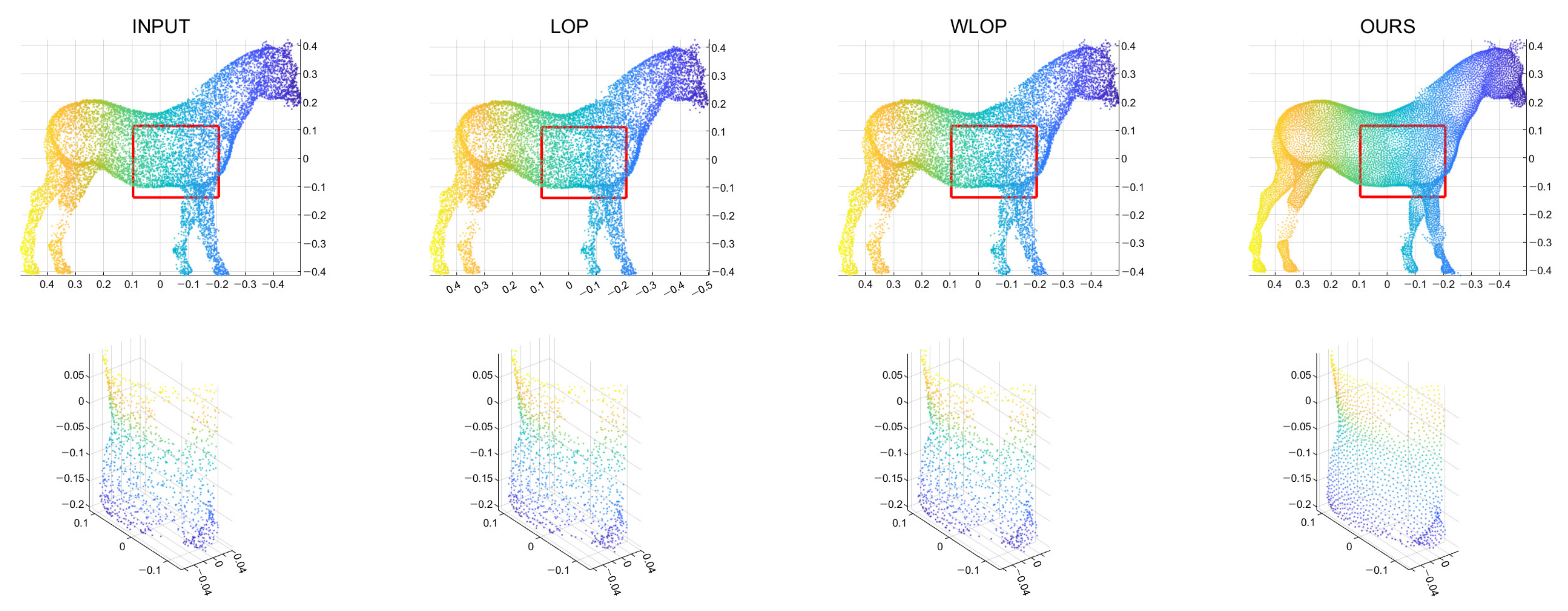
Figure 9.
Hole-filling results for the tangential directional noise case (Horse). First column: input point cloud with holes and tangential noise; second column: LOP; third column: WLOP; and fourth column: proposed method. The second row shows enlarged views of the first row.
Figure 9.
Hole-filling results for the tangential directional noise case (Horse). First column: input point cloud with holes and tangential noise; second column: LOP; third column: WLOP; and fourth column: proposed method. The second row shows enlarged views of the first row.
Figure 10.
Quantitative results for the tangential noise cases with resampling ratio 0.5. Each column represents different input data (first column: Horse; second column: Bunny; third column: Kitten; fourth column: Buddha; and fifth column: Armadillo).
Figure 10.
Quantitative results for the tangential noise cases with resampling ratio 0.5. Each column represents different input data (first column: Horse; second column: Bunny; third column: Kitten; fourth column: Buddha; and fifth column: Armadillo).
Figure 11.
Qualitative results for a tangential noise case with resampling ratio 0.5 (Horse). First column: input point cloud; second column: LOP; third column: WLOP; and fourth column: the proposed method. The second row shows enlarged views of the first row.
Figure 11.
Qualitative results for a tangential noise case with resampling ratio 0.5 (Horse). First column: input point cloud; second column: LOP; third column: WLOP; and fourth column: the proposed method. The second row shows enlarged views of the first row.
Figure 12.
Quantitative results for the omnidirectional noise cases with resampling ratio 0.5. Each column represents different input data (first column: Horse; second column: Bunny; third column: Kitten; fourth column: Buddha; and fifth column: Armadillo).
Figure 12.
Quantitative results for the omnidirectional noise cases with resampling ratio 0.5. Each column represents different input data (first column: Horse; second column: Bunny; third column: Kitten; fourth column: Buddha; and fifth column: Armadillo).
Figure 13.
Qualitative results for an omnidirectional noise case with resampling ratio 0.5 (Horse). First column: input point cloud; second column: LOP; third column: WLOP; and fourth column: the proposed method. The second row shows enlarged views of the first row.
Figure 13.
Qualitative results for an omnidirectional noise case with resampling ratio 0.5 (Horse). First column: input point cloud; second column: LOP; third column: WLOP; and fourth column: the proposed method. The second row shows enlarged views of the first row.
Figure 14.
Quantitative results for the tangential noise cases with resampling ratio 2.0. Each column represents different input data (first column: Horse; second column: Bunny; third column: Kitten; fourth column: Buddha; and fifth column: Armadillo).
Figure 14.
Quantitative results for the tangential noise cases with resampling ratio 2.0. Each column represents different input data (first column: Horse; second column: Bunny; third column: Kitten; fourth column: Buddha; and fifth column: Armadillo).
Figure 15.
Qualitative results for an tangential noise case with resampling ratio 2.0 (Horse). First column: input point cloud; second column: LOP; third column: WLOP; and fourth column: the proposed method. The second row shows enlarged views of the first row.
Figure 15.
Qualitative results for an tangential noise case with resampling ratio 2.0 (Horse). First column: input point cloud; second column: LOP; third column: WLOP; and fourth column: the proposed method. The second row shows enlarged views of the first row.
Figure 16.
Quantitative results for the omnidirectional noise cases with resampling ratio 2.0. Each column represents different input data (first column: Horse; second column: Bunny; third column: Kitten; fourth column: Buddha; and fifth column: Armadillo).
Figure 16.
Quantitative results for the omnidirectional noise cases with resampling ratio 2.0. Each column represents different input data (first column: Horse; second column: Bunny; third column: Kitten; fourth column: Buddha; and fifth column: Armadillo).
Figure 17.
Qualitative results for an omnidirectional noise case with resampling ratio 2.0 (Horse). First column: input point cloud; second column: LOP; third column: WLOP; and fourth column: the proposed method. The second row shows enlarged views of the first row.
Figure 17.
Qualitative results for an omnidirectional noise case with resampling ratio 2.0 (Horse). First column: input point cloud; second column: LOP; third column: WLOP; and fourth column: the proposed method. The second row shows enlarged views of the first row.
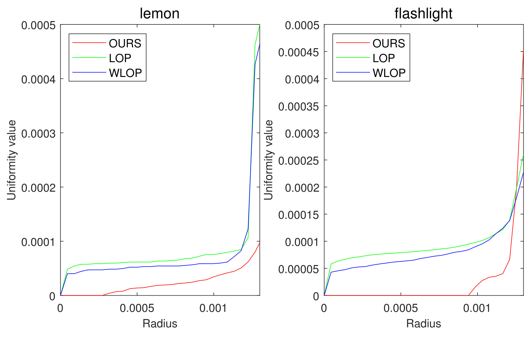
Figure 18.
Quantitative result for real data sets. The first and second columns show the uniformity results of each algorithm for Lemon and Flashlight.
Figure 18.
Quantitative result for real data sets. The first and second columns show the uniformity results of each algorithm for Lemon and Flashlight.
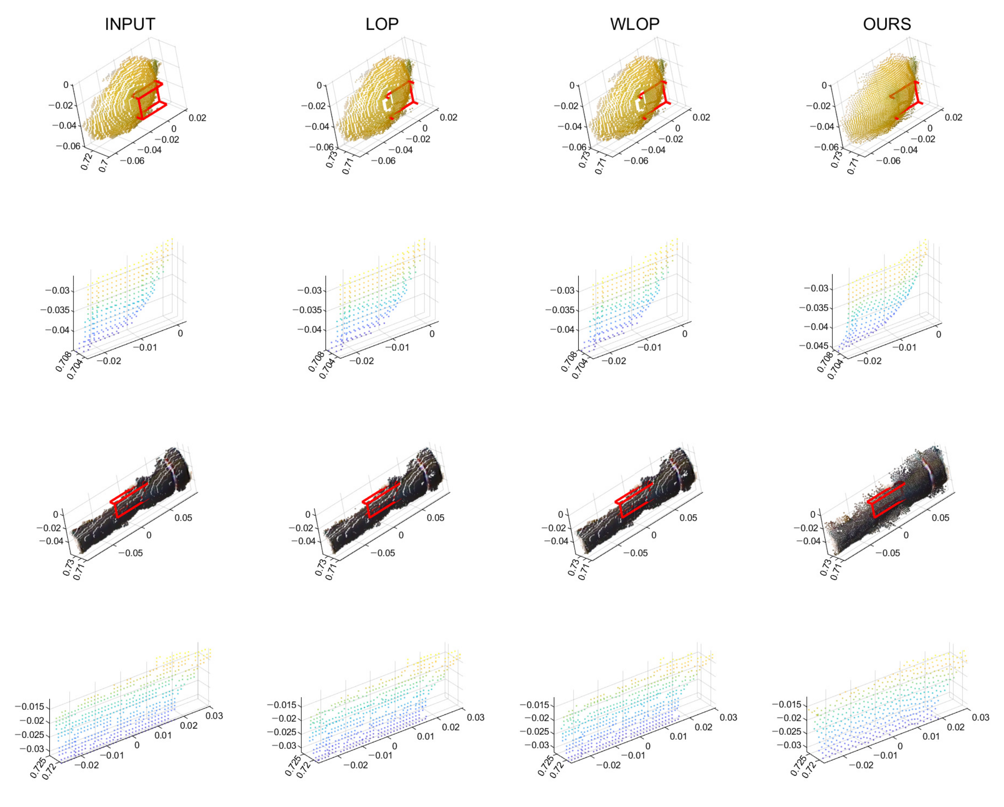
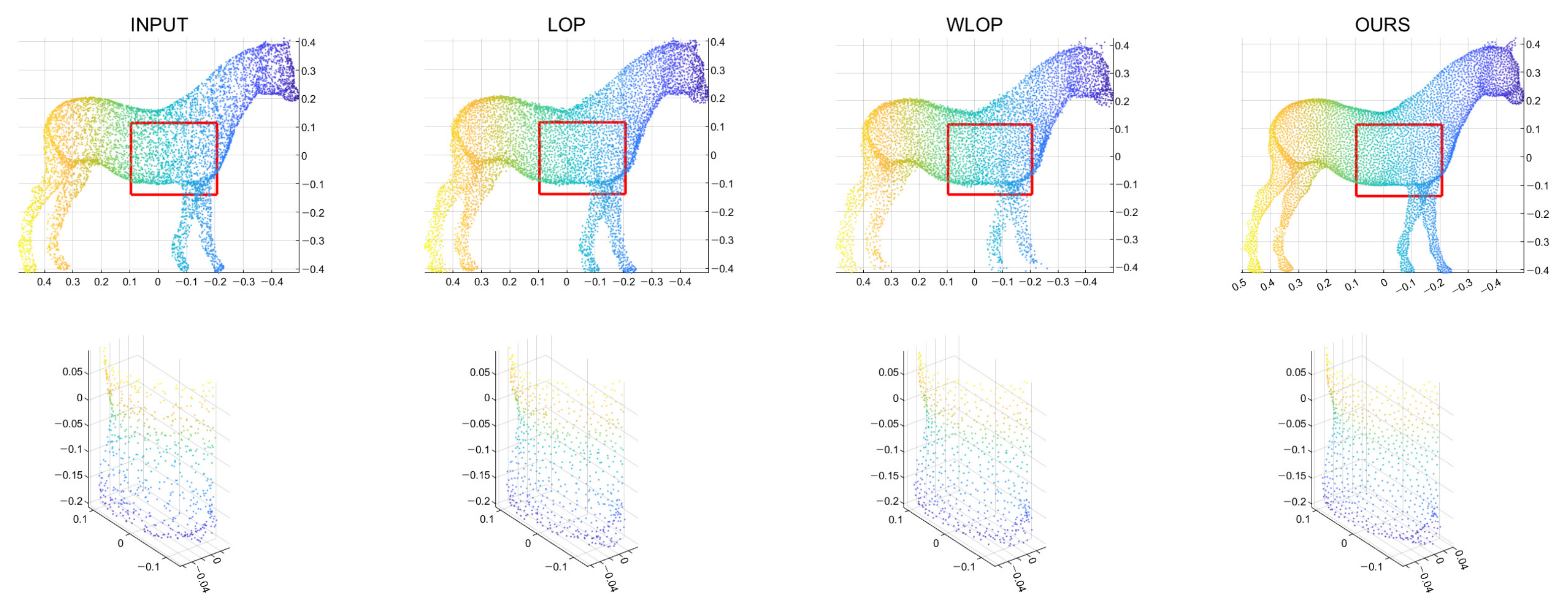
Figure 19.
Qualitative results for real data sets. The first row shows the resampled results of Lemon. The second row shows enlarged views of the first row. The third row shows the resampled results of Flashlight. The fourth row shows enlarged views of the third row. First column: input point cloud; second column: LOP; third column: WLOP; and fourth column: proposed method.
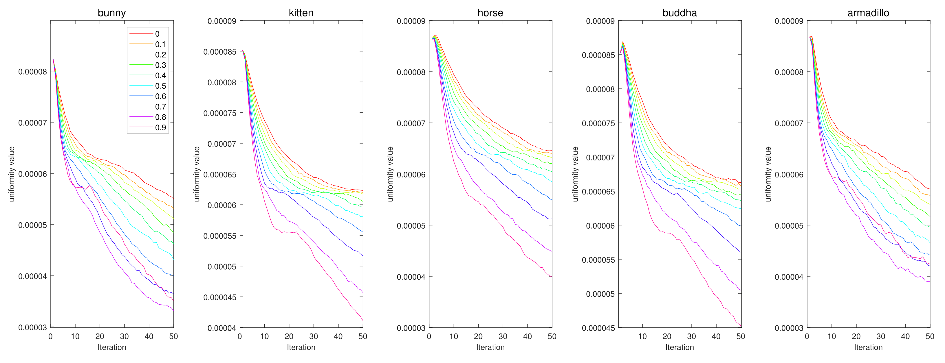
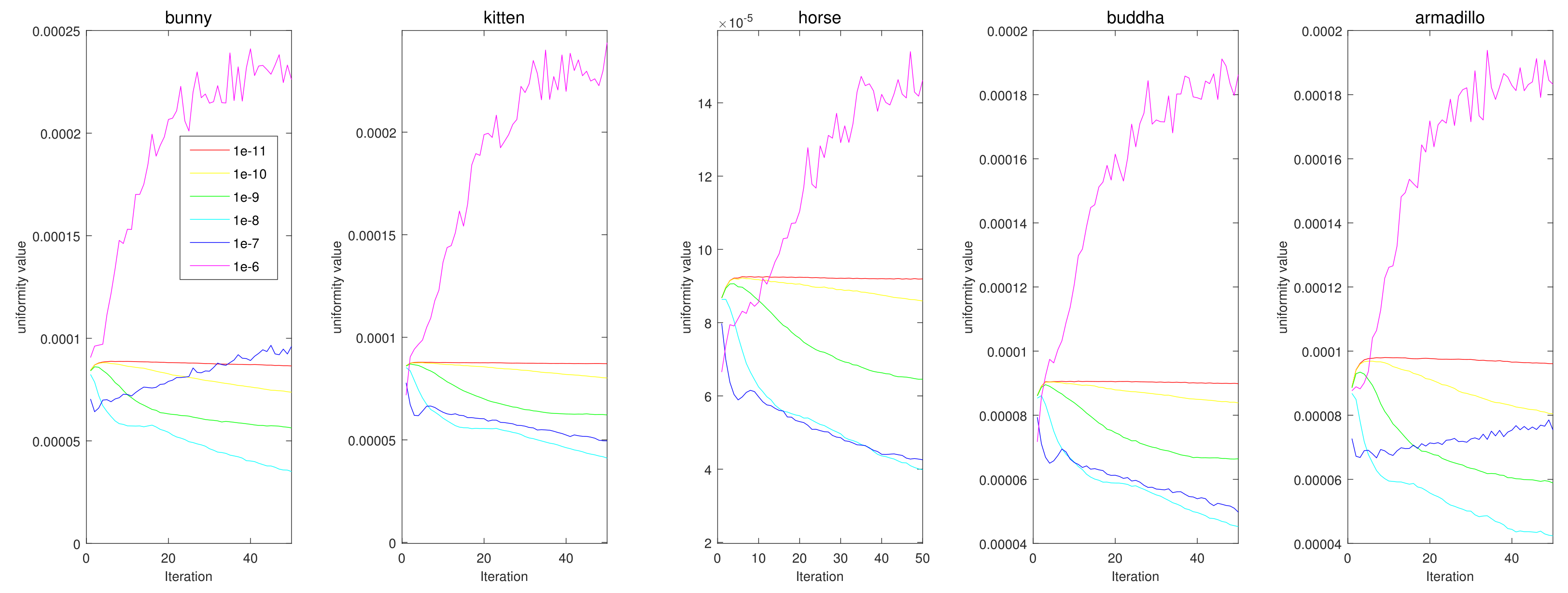
Figure 20.
Quantitative performance of the proposed method for various . The horizontal axis indicates the iteration, and the vertical axis indicates the uniformity value. Each column represents a different input point cloud (first column: Horse, second column: Bunny, third column: Kitten, fourth column: Buddha, and fifth column: Armadillo).
Figure 21.
Quantitative performance of the proposed method for various . The horizontal axis indicates the iteration, and the vertical axis indicates the uniformity value. Each column represents a different input point cloud (first column: Horse, second column: Bunny, third column: Kitten, fourth column: Buddha, and fifth column: Armadillo).
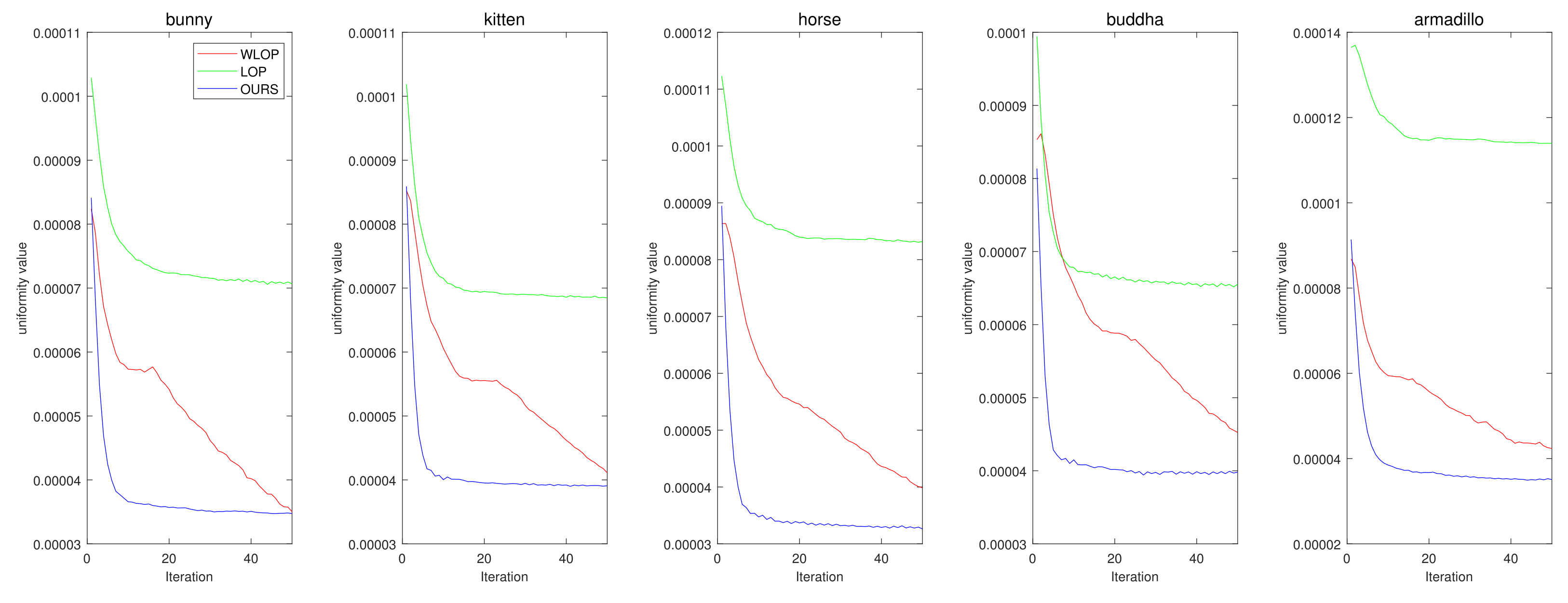
Figure 22.
Convergence results of compared methods for the resampling experiment with tangential case. (first column: Horse, second column: Bunny, third column: Kitten, fourth column: Buddha, and fifth column: Armadillo).
Figure 22.
Convergence results of compared methods for the resampling experiment with tangential case. (first column: Horse, second column: Bunny, third column: Kitten, fourth column: Buddha, and fifth column: Armadillo).
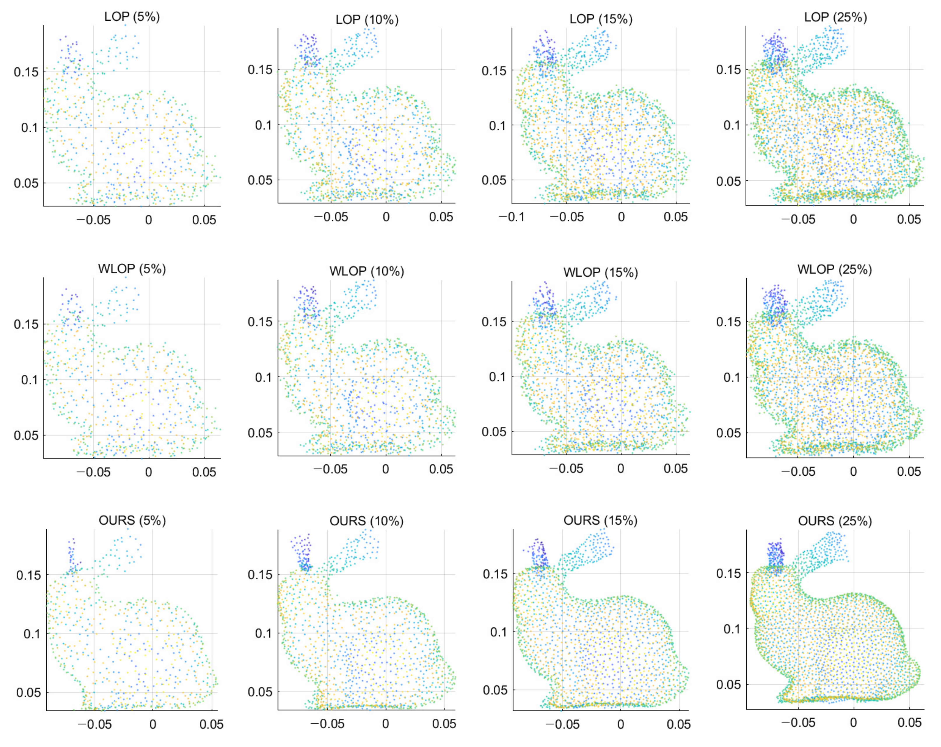
Figure 23.
Resampling results of low-density inputs. The input point clouds were generated by randomly subsampling the input data of
Figure 5. The percentages in the parentheses represent the amount of subsampling. First row: LOP, second row: WLOP, and third row: proposed method.
Figure 23.
Resampling results of low-density inputs. The input point clouds were generated by randomly subsampling the input data of
Figure 5. The percentages in the parentheses represent the amount of subsampling. First row: LOP, second row: WLOP, and third row: proposed method.
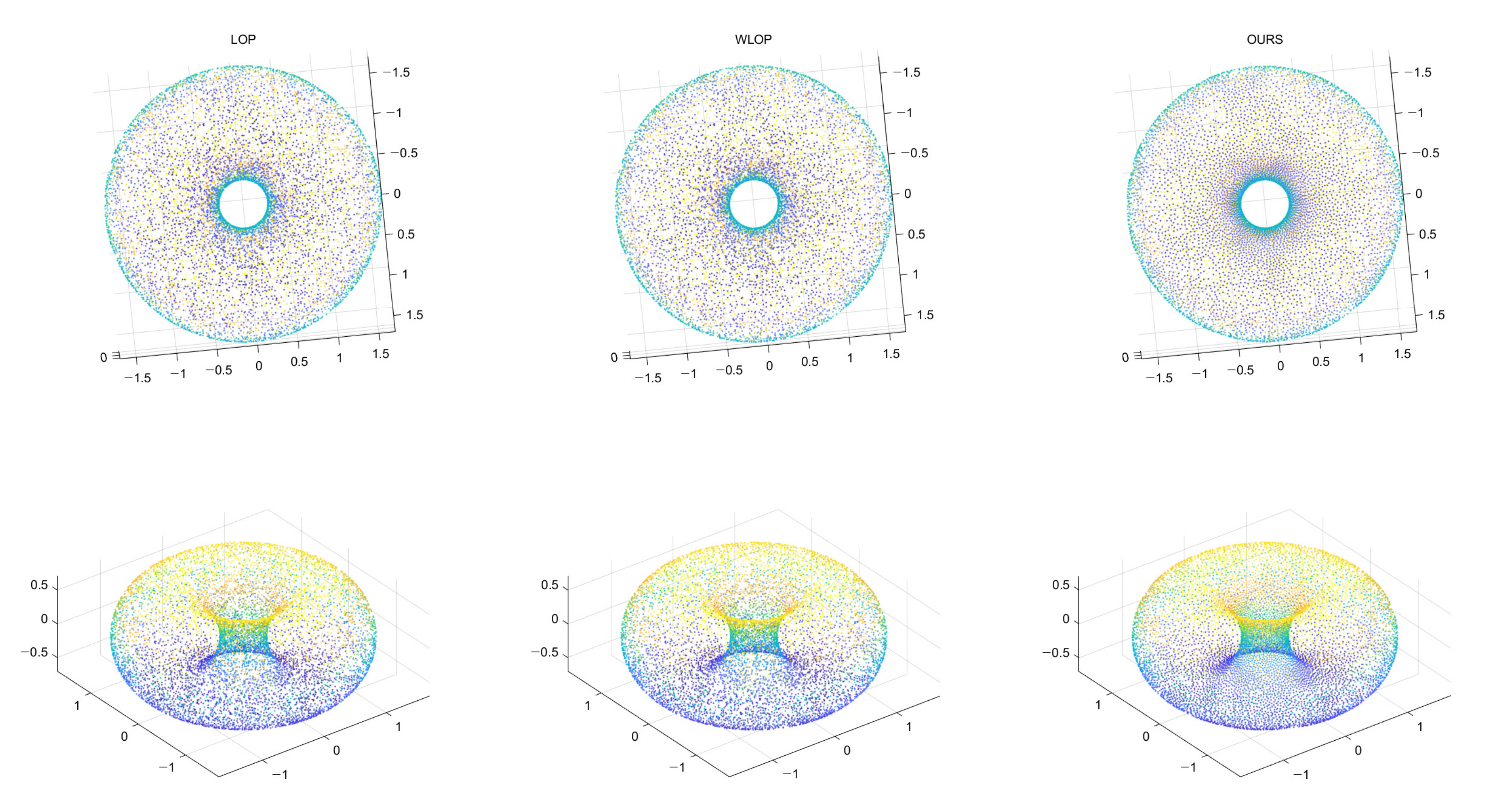
Figure 24.
Resampling result of a genus-one shape. Left: LOP, middle: WLOP, and right: proposed method.
Figure 24.
Resampling result of a genus-one shape. Left: LOP, middle: WLOP, and right: proposed method.
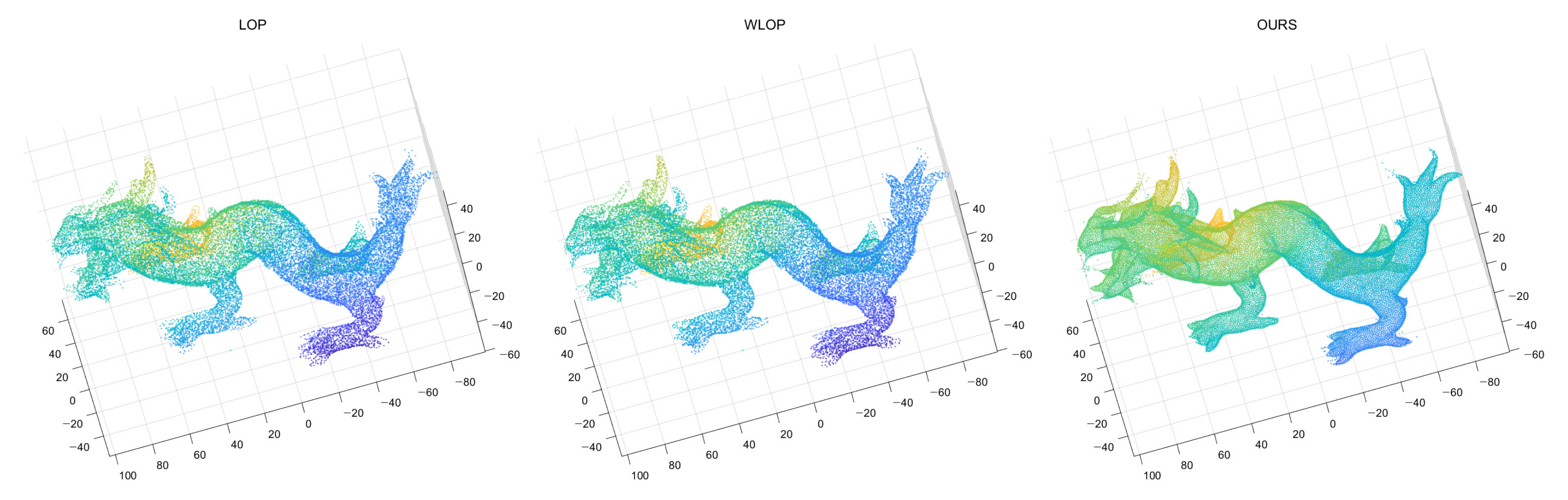
Figure 25.
Resampling results of Dragon. (Left): LOP, (Middle): WLOP, (Right): proposed method.
Figure 25.
Resampling results of Dragon. (Left): LOP, (Middle): WLOP, (Right): proposed method.
Table 1.
Running times of different algorithms for various input data and resampling ratios. The best results are highlighted in bold.
Table 1.
Running times of different algorithms for various input data and resampling ratios. The best results are highlighted in bold.
| Resampling Ratio | Method | Horse | Bunny | Kitten | Buddaha | Armadilo |
|---|
| 0.5 (Subsampling) | LOP | 112.35 s | 57.81 s | 96.84 s | 108.57 s | 112.89 s |
| WLOP | 156.98 s | 144.96 s | 153.67 s | 141.39 s | 118.76 s |
| ours | 73.97 s | 75.52 s | 74.73 s | 55.61 s | 54.96 s |
| 1.0 (Resampling) | LOP | 435.17 s | 424.60 s | 437.59 s | 406.28 s | 296.43 s |
| WLOP | 585.16 s | 559.99 s | 584.19 s | 549.82 s | 428.72 s |
| ours | 108.24 s | 112.36 s | 111.71 s | 105.53 s | 107.21 s |
| 2.0 (Upsampling) | LOP | 752.24 s | 763.53 s | 748.47 s | 705.54 s | 743.19 s |
| WLOP | 1150.53 s | 1030.98 s | 1083.53 s | 1101.86 s | 1119.77 s |
| ours | 284.78 s | 219.58 s | 237.51 s | 254.56 s | 280.32 s |


