
Dual-Input and Multi-Channel Convolutional Neural Network Model for Vehicle Speed Prediction


Abstract
:1. Introduction
- (1)
- Deep learning models are used to build the speed prediction model. The deep architecture has more tunable parameters, which can lead to better prediction results.
- (2)
- The training set is constructed based on rich vehicle data obtained from road experiments. The various vehicle signal sequences provide a more detailed picture of the current operating status of the vehicle.
- (3)
- The second type of input for the model characterizes the pedal signal. As a direct representation of driver intent in vehicle signals, the second type of input enables the prediction model to more sensitively capture trends in vehicle speed changes.
2. Road Experiments
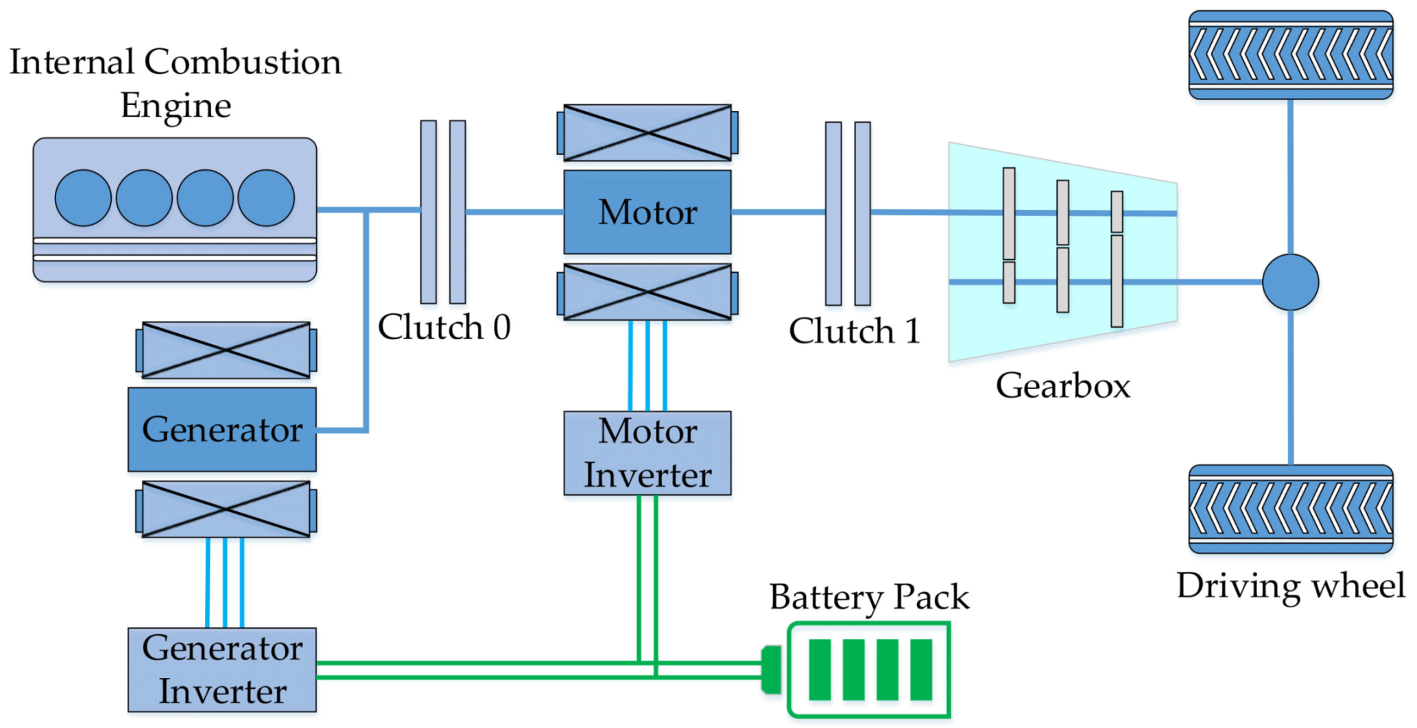
2.1. Vehicle Model
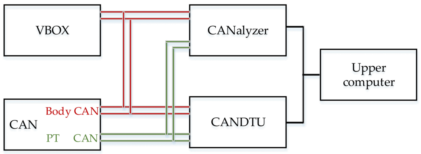
2.2. Experiment Method
2.3. Data Processing
| Algorithm 1. Recursive mean filter | |
| Data: origin signal vector , vector length , window length | |
| Result: filtered signal vector | |
| 1 | for to do |
| 2 | if then break |
| 3 | Else then mean() |
| 4 | end |
| 5 | end |
3. Speed Prediction Model
3.1. CNN
3.1.1. Convolution Layer
3.1.2. Batch Normalization Layer
3.1.3. Activation Layer
3.1.4. Pooling Layer
3.1.5. Fully Connected Layer
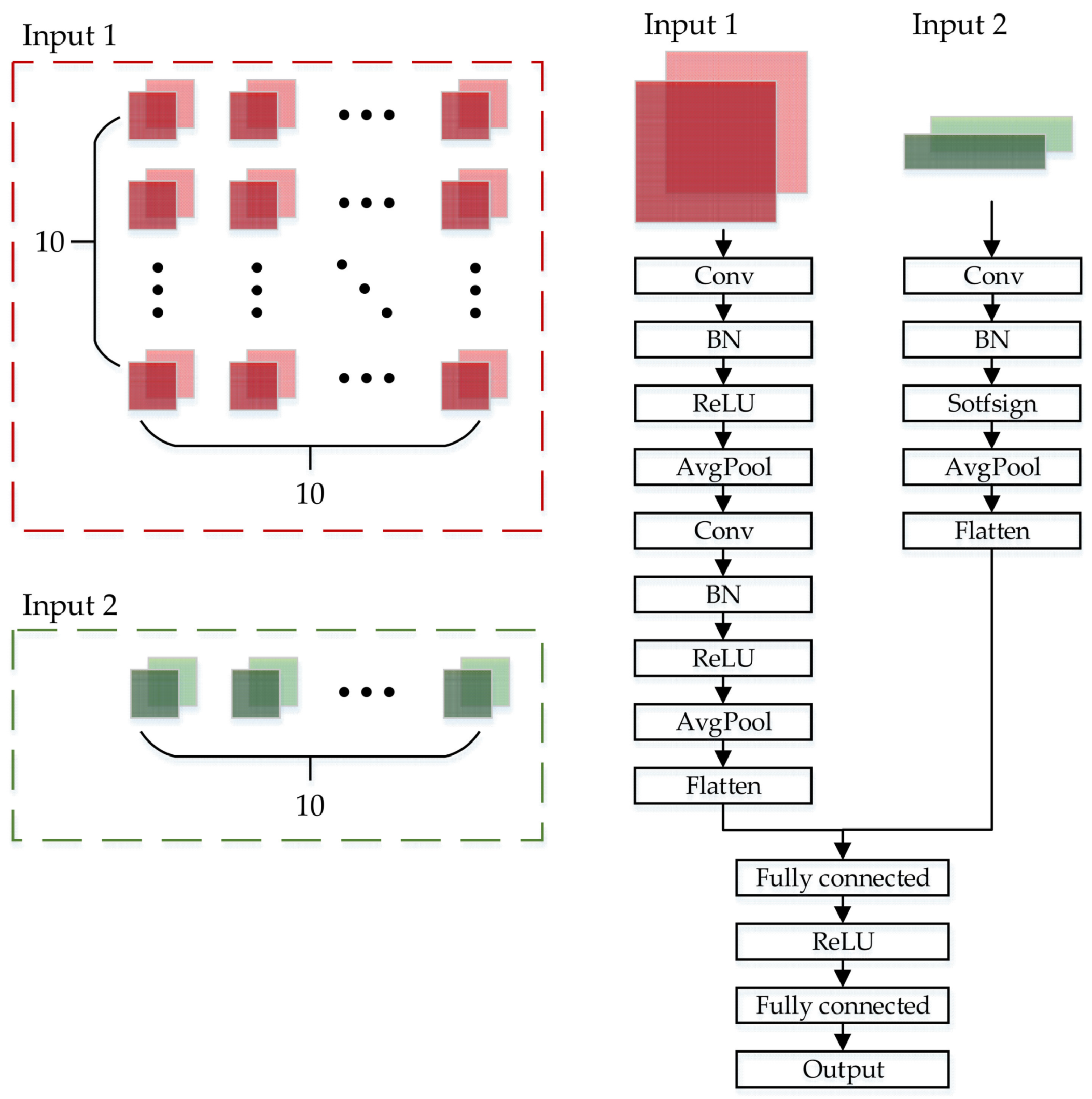
3.2. The Architecture of DICNN
4. Energy Management Strategy
4.1. Fundamentals of ECMS
4.2. ECMS with Speed Prediction
5. Validation
5.1. Preformance Evaluation
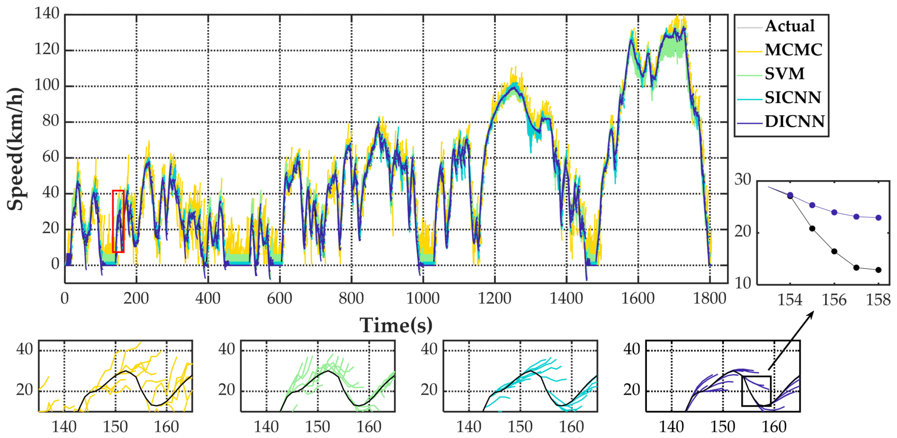
5.2. Simulation
6. Conclusions
Author Contributions
Funding
Conflicts of Interest
References
- Nie, H.; Cui, N.X.; Du, Y.; Wang, M. An Improved Velocity Forecasts Method Considering the Speed and Following Distance of Two Vehicles. In Proceedings of the 39th Chinese Control Conference (CCC), Shenyang, China, 27–29 July 2020; pp. 5517–5522. [Google Scholar]
- Jiang, B.N.; Fei, Y.S. Vehicle Speed Prediction by Two-Level Data Driven Models in Vehicular Networks. IEEE Trans. Intell. Transp. Syst. 2017, 18, 1793–1801. [Google Scholar] [CrossRef]
- Li, Y.F.; Chen, M.N.; Zhao, W.Z. Investigating long-term vehicle speed prediction based on BP-LSTM algorithms. IET Intell. Transp. Syst. 2019, 13, 1281–1290. [Google Scholar] [CrossRef]
- Li, Y.F.; Chen, M.N.; Lu, X.D.; Zhao, W.Z. Research on optimized GA-SVM vehicle speed prediction model based on driver-vehicle-road-traffic system. Sci. China-Technol. Sci. 2018, 61, 782–790. [Google Scholar] [CrossRef]
- Yeon, K.; Min, K.; Shin, J.; Sunwoo, M.; Han, M. Ego-Vehicle Speed Prediction Using a Long Short-Term Memory Based Recurrent Neural Network. Int. J. Automot. Technol. 2019, 20, 713–722. [Google Scholar] [CrossRef]
- Zhang, L.S.; Zhang, J.Y.; Liu, D.Q.; IEEE. Neural Network based Vehicle Speed Prediction for Specific Urban Driving. In Proceedings of the Chinese Automation Congress (CAC), Xi’an, China, 30 November–2 December 2018; pp. 1798–1803. [Google Scholar]
- Ghandour, R.; da Cunha, F.H.R.; Victorino, A.; Charara, A.; Lechner, D.; IEEE. A method of vehicle dynamics prediction to anticipate the risk of future accidents: Experimental validation. In 2011 14th International IEEE Conference on Intelligent Transportation Systems; IEEE International Conference on Intelligent Transportation Systems-ITSC; IEEE: New York, NY, USA, 2011; pp. 1692–1697. [Google Scholar]
- Ma, Z.Y.; Zhang, Y.Q.; Yang, J. Velocity and normal tyre force estimation for heavy trucks based on vehicle dynamic simulation considering the road slope angle. Veh. Syst. Dyn. 2016, 54, 137–167. [Google Scholar] [CrossRef]
- Magliolo, M.; Bacchi, M.; Sacone, S.; Siri, S.; IEEE. Traffic Mean Speed Evaluation in Freeway Systems; IEEE: New York, NY, USA, 2004; pp. 233–238. [Google Scholar]
- Bie, Y.W.; Qiu, T.Z.; Zhang, C.; Zhang, C.B. Introducing Weather Factor Modelling into Macro Traffic State Prediction. J. Adv. Transp. 2017, 2017, 4879170. [Google Scholar] [CrossRef] [Green Version]
- Zhang, S.N.; Wu, D.A.; Wu, L.; Lu, Y.B.; Peng, J.Y.; Chen, X.Y.; Ye, A.D.; IEEE. A Markov Chain Model with High-Order Hidden Process and Mixture Transition Distribution. In Proceedings of the International Conference on Cloud Computing and Big Data (CLOUDCOM-ASIA), Fuzhou, China, 16–18 December 2013; pp. 509–514. [Google Scholar]
- Liu, H.; Chen, C.; Lv, X.W.; Wu, X.; Liu, M. Deterministic wind energy forecasting: A review of intelligent predictors and auxiliary methods. Energy Convers. Manag. 2019, 195, 328–345. [Google Scholar] [CrossRef]
- Schmidhuber, J. Deep learning in neural networks: An overview. Neural Netw. 2015, 61, 85–117. [Google Scholar] [CrossRef] [PubMed] [Green Version]
- Shin, J.; Kim, S.; Sunwoo, M.; Han, M.; IEEE. Ego-Vehicle Speed Prediction Using Fuzzy Markov Chain With Speed Constraints. In 2019 30th IEEE Intelligent Vehicles Symposium; IEEE Intelligent Vehicles Symposium; IEEE: New York, NY, USA, 2019; pp. 2106–2112. [Google Scholar]
- Zhou, Y.; Ravey, A.; Pera, M.C.; IEEE. A Velocity Prediction Method based on Self-Learning Multi-Step Markov Chain. In 45th Annual Conference of the IEEE Industrial Electronics Society; IEEE Industrial Electronics Society; IEEE: New York, NY, USA, 2019; pp. 2598–2603. [Google Scholar]
- Zhang, L.P.; Liu, W.; Qi, B.N. Combined Prediction for Vehicle Speed with Fixed Route. Chin. J. Mech. Eng. 2020, 33, 60. [Google Scholar] [CrossRef]
- Li, Y.F.; Zhang, J.; Ren, C.; Lu, X.D. Prediction of vehicle energy consumption on a planned route based on speed features forecasting. IET Intell Transp Syst. 2020, 14, 511–522. [Google Scholar]
- Mozaffari, L.; Mozaffari, A.; Azad, N.L. Vehicle speed prediction via a sliding-window time series analysis and an evolutionary least learning machine: A case study on San Francisco urban roads. Eng. Sci. and Technol.—Int. J.-Jestech 2015, 18, 150–162. [Google Scholar] [CrossRef] [Green Version]
- He, H.W.; Wang, Y.L.; Han, R.Y.; Han, M.; Bai, Y.F.; Liu, Q.W. An improved MPC-based energy management strategy for hybrid vehicles using V2V and V2I communications. Energy 2021, 225, 120273. [Google Scholar] [CrossRef]
- Song, C.; Lee, H.; Kang, C.; Lee, W.; Kim, Y.B.; Cha, S.W.; IEEE. Traffic Speed Prediction under Weekday Using Convolutional Neural Networks Concepts. In 2017 28th IEEE Intelligent Vehicles Symposium; IEEE Intelligent Vehicles Symposium; IEEE: New York, NY, USA, 2017; pp. 1293–1298. [Google Scholar]
- Han, S.J.; Zhang, F.Q.; Xi, J.Q.; Ren, Y.F.; Xu, S.H.; IEEE. Short-term Vehicle Speed Prediction Based on Convolutional Bidirectional LSTM Networks. In 2019 IEEE Intelligent Transportation Systems Conference; IEEE International Conference on Intelligent Transportation Systems-ITSC; IEEE: New York, NY, USA, 2019; pp. 4055–4060. [Google Scholar]
- Zhang, B.D.; Yang, F.Y.; Teng, L.; Ouyang, M.G.; Guo, K.F.; Li, W.F.; Du, J.Y. Comparative Analysis of Technical Route and Market Development for Light-Duty PHEV in China and the US. Energies 2019, 12, 23. [Google Scholar] [CrossRef]
- Zhou, X.Y.; Qin, D.; Hu, J.J. Multi-objective optimization design and performance evaluation for plug-in hybrid electric vehicle powertrains. Appl. Energy 2017, 208, 1608–1625. [Google Scholar] [CrossRef]
- Li, X.M.; Liu, H.; Wang, W.D. Mode Integration Algorithm Based Plug-In Hybrid Electric Vehicle Energy Management Strategy Research. In Proceedings of the 8th International Conference on Applied Energy (ICAE), Beijing Inst Technol, Beijing, China, 8–11 October 2016; pp. 2647–2652. [Google Scholar]
- Memon, R.A.; Khaskheli, G.B.; Dahani, M.A. Estimation of operating speed on two lane two way roads along N-65 (SIBI -Quetta). Int. J. Civ. Eng. 2012, 10, 25–31. [Google Scholar]
- Zhang, X.B.; Xu, L.F.; Li, J.Q.; Ouyang, M.G.; IEEE. Real-time estimation of vehicle mass and road grade based on multi-sensor data fusion. In Proceedings of the 9th IEEE Vehicle Power and Propulsion Conference (VPPC), Beijing, China, 15–18 October 2013; pp. 486–492. [Google Scholar]
- Zhang, Q.R.; Zhang, M.; Chen, T.H.; Sun, Z.F.; Ma, Y.Z.; Yu, B. Recent advances in convolutional neural network acceleration. Neurocomputing 2019, 323, 37–51. [Google Scholar] [CrossRef] [Green Version]
- Kolarik, M.; Burget, R.; Riha, K. Comparing Normalization Methods for Limited Batch Size Segmentation Neural Networks. In Proceedings of the 43rd International Conference on Telecommunications and Signal Processing (TSP), Electr Network, Milan, Italy, 7–9 July 2020; pp. 677–680. [Google Scholar]
- Hu, Z.; Li, Y.P.; Yang, Z.Y.; IEEE. Improving Convolutional Neural Network Using Pseudo Derivative ReLU. In Proceedings of the 5th International Conference on Systems and Informatics (ICSAI), Nanjing, China, 10–12 November 2018; pp. 283–287. [Google Scholar]
- Chang, C.H.; Zhang, E.H.; Huang, S.H.; IEEE. Softsign Function Hardware Implementation Using Piecewise Linear Approximation. In Proceedings of the International Symposium on Intelligent Signal Processing and Communication Systems (lSPACS), Taipei, Taiwan, 3–6 December 2019. [Google Scholar]
- Xie, Y.; Savvaris, A.; Tsourdos, A. Fuzzy logic based equivalent consumption optimization of a hybrid electric propulsion system for unmanned aerial vehicles. Aerosp. Sci. Technol. 2019, 85, 13–23. [Google Scholar] [CrossRef] [Green Version]
- Rezaei, A.; Burl, J.B.; Zhou, B. Estimation of the ECMS Equivalent Factor Bounds for Hybrid Electric Vehicles. IEEE Trans. Control Syst. Technol. 2018, 26, 2198–2205. [Google Scholar] [CrossRef]
- Liu, L.Z.; Zhang, B.Z.; Liang, H.Y. Global Optimal Control Strategy of PHEV Based on Dynamic Programming. In Proceedings of the 6th International Conference on Information Science and Control Engineering (ICISCE), Shanghai, China, 20–22 December 2019; pp. 758–762. [Google Scholar]


| Component | Parameter | Value | Unit |
|---|---|---|---|
| Vehicle | Vehicle weight | 1200 | kg |
| Tire radius | 0.323 | m | |
| Final drive ratio | 4.021 | / | |
| Engine | Maximum torque | 165 | Nm |
| Maximum power | 105@6500 | kW@rpm | |
| Motor | Maximum torque | 307 | Nm |
| Maximum power | 126@12584 | kW@rpm | |
| Battery | Rated capacity | 20.8 | Ah |
| Rated voltage | 366 | V | |
| Gear | First | 3.527 | / |
| Second | 2.025 | / | |
| Third | 1.382 | / | |
| Fourth | 1.058 | / | |
| Fifth | 0.958 | / |
| Knot | Signal | Source | Frequency |
|---|---|---|---|
| VCU | VCU vehicle speed | PT CAN | 100 Hz |
| Drive pedal opening | PT CAN | 100 Hz | |
| Brake pedal opening | PT CAN | 100 Hz | |
| ABS | ABS vehicle speed | Body CAN | 100 Hz |
| VBOX | Latitude | Body CAN | 100 Hz |
| Longitude | Body CAN | 100 Hz | |
| VBOX vehicle speed | Body CAN | 100 Hz | |
| longitudinal acceleration | Body CAN | 100 Hz | |
| MCU | Motor speed | PT CAN | 100 Hz |
| Motor torque | PT CAN | 100 Hz | |
| DC bus voltage | PT CAN | 100 Hz | |
| DC bus current | PT CAN | 100 Hz | |
| ECU | Engine speed | PT CAN | 100 Hz |
| Engine torque | PT CAN | 100 Hz | |
| BMS | State of charge | PT CAN | 10 Hz |
| BMS voltage | PT CAN | 10 Hz | |
| BMS current | PT CAN | 10 Hz |
| Method | Prediction Time (s) | ||||
|---|---|---|---|---|---|
| 1s | 2s | 3s | 4s | 5s | |
| MCMC | 4.12 | 6.33 | 8.25 | 9.96 | 11.63 |
| SVM | 1.81 | 2.41 | 3.66 | 4.71 | 7.08 |
| SICNN | 1.36 | 2.74 | 4.28 | 5.91 | 7.49 |
| DICNN | 0.81 | 1.83 | 3.07 | 4.41 | 5.75 |
| Method | Prediction Time (s) | ||||
|---|---|---|---|---|---|
| 1s | 2s | 3s | 4s | 5s | |
| MCMC | 3.00 | 4.70 | 6.26 | 7.59 | 8.88 |
| SVM | 1.48 | 1.76 | 2.80 | 3.47 | 5.70 |
| SICNN | 0.97 | 1.96 | 3.06 | 4.35 | 5.55 |
| DICNN | 0.48 | 1.15 | 2.02 | 2.99 | 3.99 |
| Method | Prediction Time (s) | ||||
|---|---|---|---|---|---|
| 1s | 2s | 3s | 4s | 5s | |
| MCMC | 17.97 | 27.04 | 37.12 | 36.02 | 38.72 |
| SVM | 6.15 | 12.86 | 14.27 | 21.67 | 29.67 |
| SICNN | 6.22 | 11.43 | 15.66 | 21.63 | 27.68 |
| DICNN | 5.12 | 9.03 | 14.85 | 20.87 | 25.95 |
| Method | Prediction Time (s) | ||||
|---|---|---|---|---|---|
| 1s | 2s | 3s | 4s | 5s | |
| MCMC | 0.9871 | 0.9696 | 0.9483 | 0.9246 | 0.8973 |
| SVM | 0.9975 | 0.9956 | 0.9899 | 0.9832 | 0.9619 |
| SICNN | 0.9986 | 0.9943 | 0.9861 | 0.9735 | 0.9574 |
| DICNN | 0.9995 | 0.9975 | 0.9929 | 0.9852 | 0.9749 |
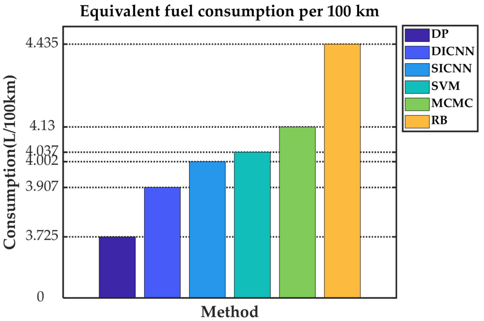
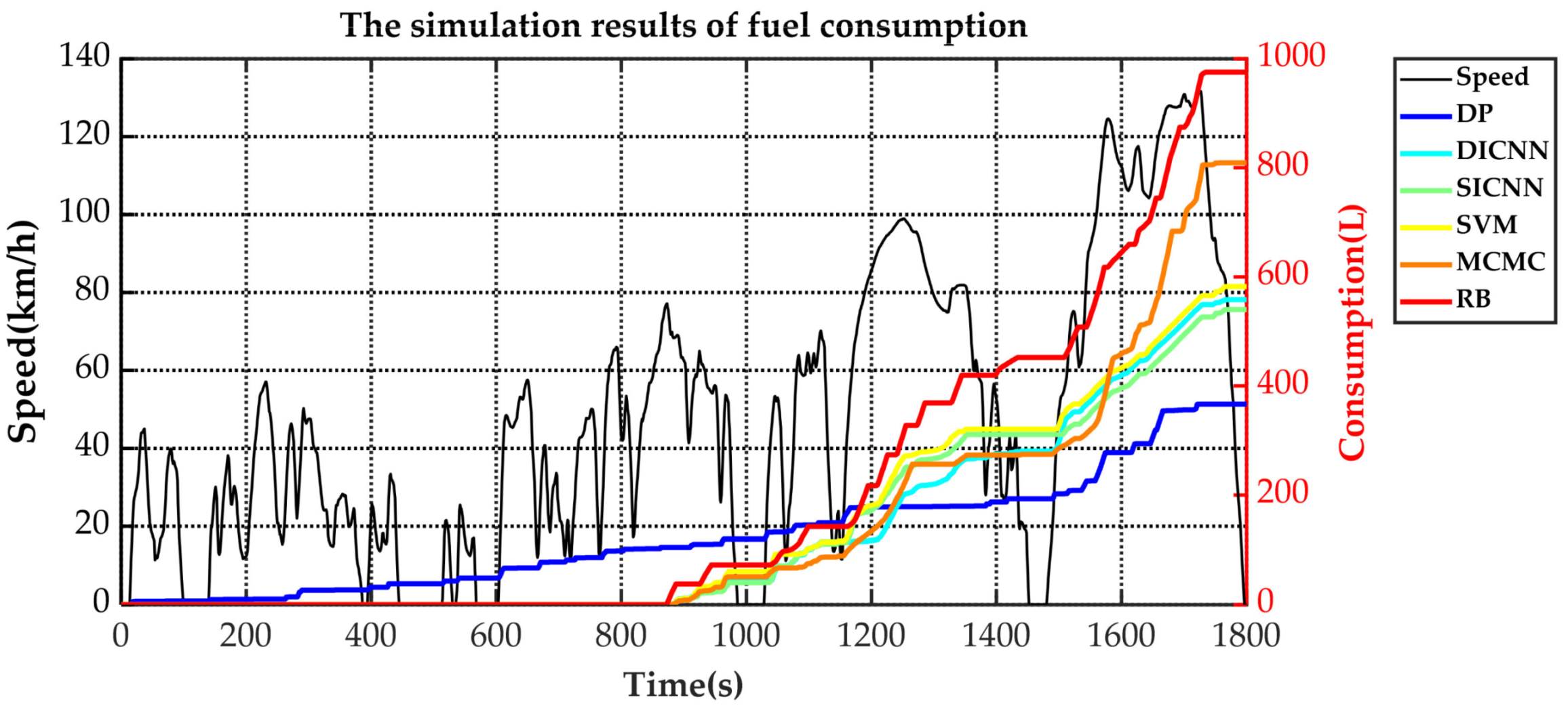
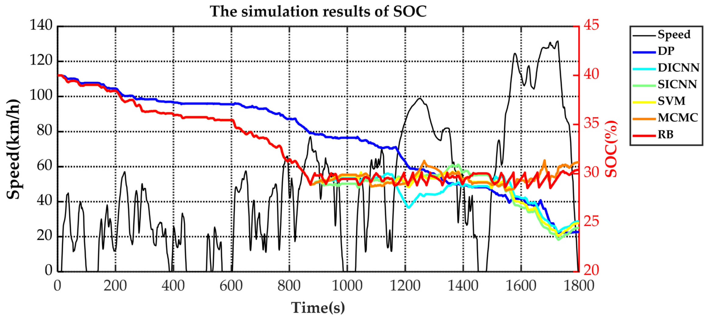
| Method | Fuel Consumption (mL) | Final SOC (%) | Equivalent Fuel Consumption (L/100 km) | Increased Equivalent Fuel Consumption Compared with DP (%) |
|---|---|---|---|---|
| DP | 366.76 | 24.05 | 3.725 | / |
| MICNN | 558.19 | 25.13 | 3.907 | 4.89 |
| SICNN | 540.21 | 24.47 | 4.002 | 7.44 |
| SVM | 582.13 | 24.96 | 4.037 | 8.38 |
| MCMC | 809.30 | 31.16 | 4.130 | 10.87 |
| RB | 975.54 | 30.38 | 4.435 | 19.06 |
Publisher’s Note: MDPI stays neutral with regard to jurisdictional claims in published maps and institutional affiliations. |
© 2021 by the authors. Licensee MDPI, Basel, Switzerland. This article is an open access article distributed under the terms and conditions of the Creative Commons Attribution (CC BY) license (https://creativecommons.org/licenses/by/4.0/).
Share and Cite
Xing, J.; Chu, L.; Guo, C.; Pu, S.; Hou, Z. Dual-Input and Multi-Channel Convolutional Neural Network Model for Vehicle Speed Prediction. Sensors 2021, 21, 7767. https://doi.org/10.3390/s21227767
Xing J, Chu L, Guo C, Pu S, Hou Z. Dual-Input and Multi-Channel Convolutional Neural Network Model for Vehicle Speed Prediction. Sensors. 2021; 21(22):7767. https://doi.org/10.3390/s21227767
Chicago/Turabian StyleXing, Jiaming, Liang Chu, Chong Guo, Shilin Pu, and Zhuoran Hou. 2021. "Dual-Input and Multi-Channel Convolutional Neural Network Model for Vehicle Speed Prediction" Sensors 21, no. 22: 7767. https://doi.org/10.3390/s21227767
APA StyleXing, J., Chu, L., Guo, C., Pu, S., & Hou, Z. (2021). Dual-Input and Multi-Channel Convolutional Neural Network Model for Vehicle Speed Prediction. Sensors, 21(22), 7767. https://doi.org/10.3390/s21227767