
Human Gait Recognition: A Single Stream Optimal Deep Learning Features Fusion

 ,
,  ,
,  , , and
Abstract
:1. Introduction
- Recognizing gait in various circumstances, such as changing view angles and walking styles while still wearing a coat and bag, is a difficult challenge.
- Different subjects have their distinct gait; however, some of the subjects have a very similar gait. This issue misleads the correct classification and degrades the system’s performance.
- Some researchers follow the two step process for gait recognition, such as subject detection and then classification. However, this first step is not a guarantee for accurate recognition of human gait due to incorrect subject detection. Also, two-step process increases the computational time.
- Variation in the style of clothings such as a long coat, half shirt, skirt, regular pants, coats, and so on. In these styles, it is not easy to extract the rich features for further classification.
- The irrelevant features information which is extracted from the original frames is an impact on the system accuracy and computational time.
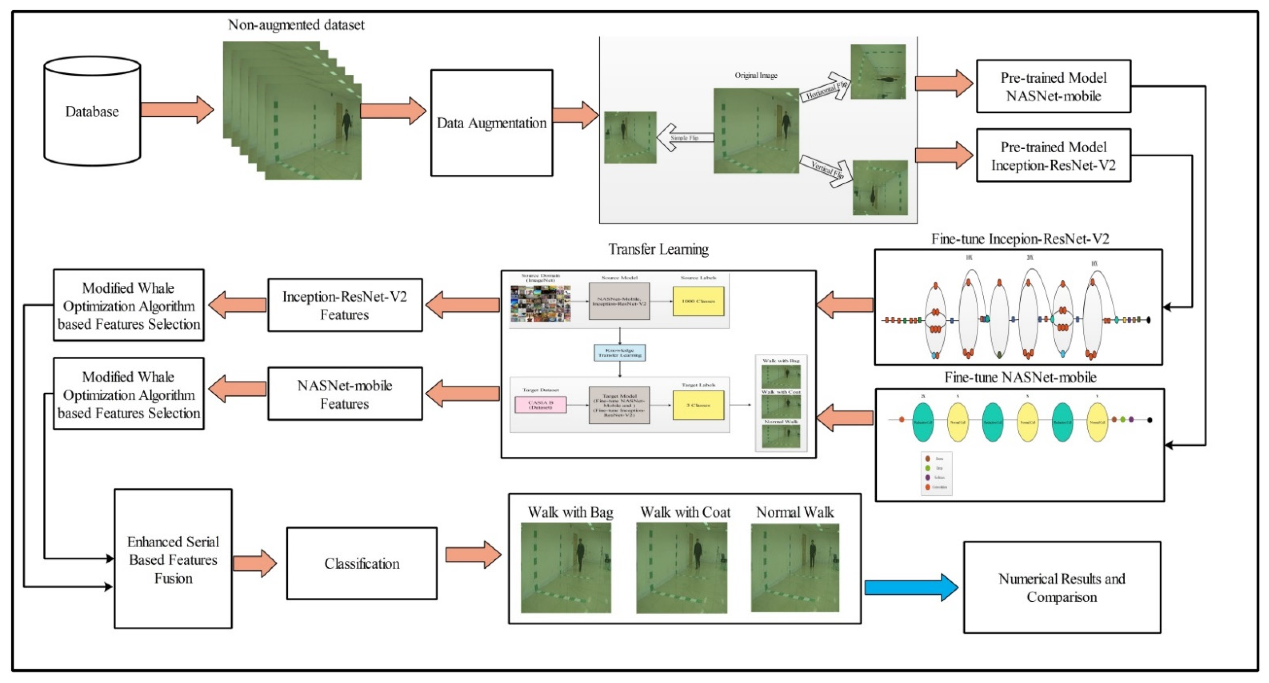
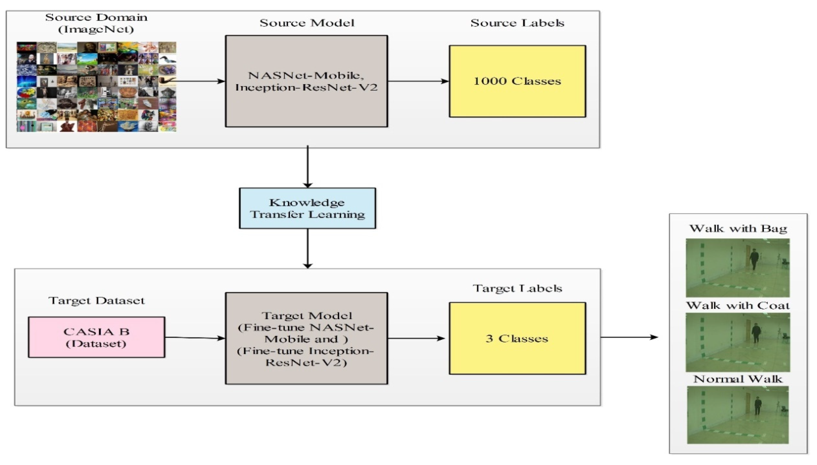
- Modified two pre-trained deep learning models on CASIA B dataset and performed transfer learning. After the transfer learning, features are extracted from the average pool layer.
- Features are fused using a modified mean absolute deviation extended serial fusion (MDeSF) approach.
- The best features are selected using a three-step Improved Whale Optimization algorithm.
2. Related Work
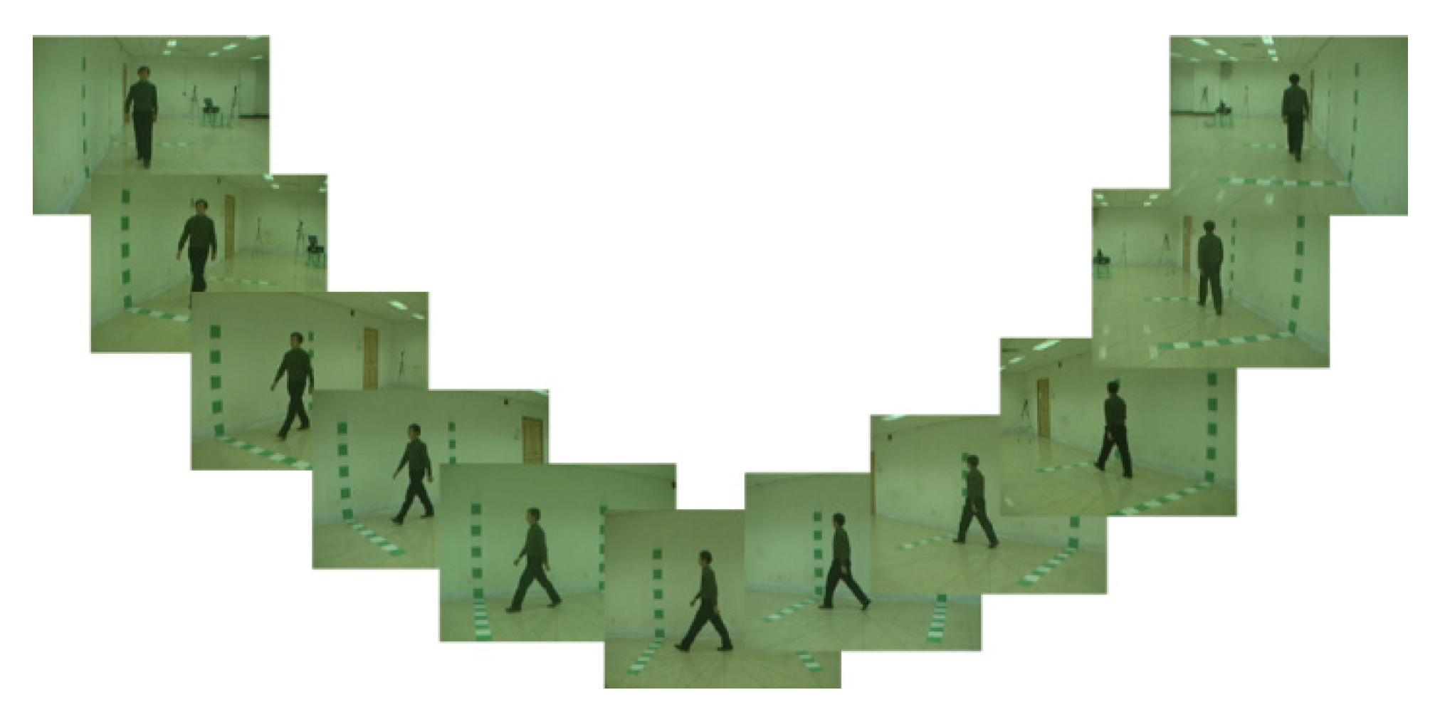
3. Dataset Detail
4. Materials and Methods
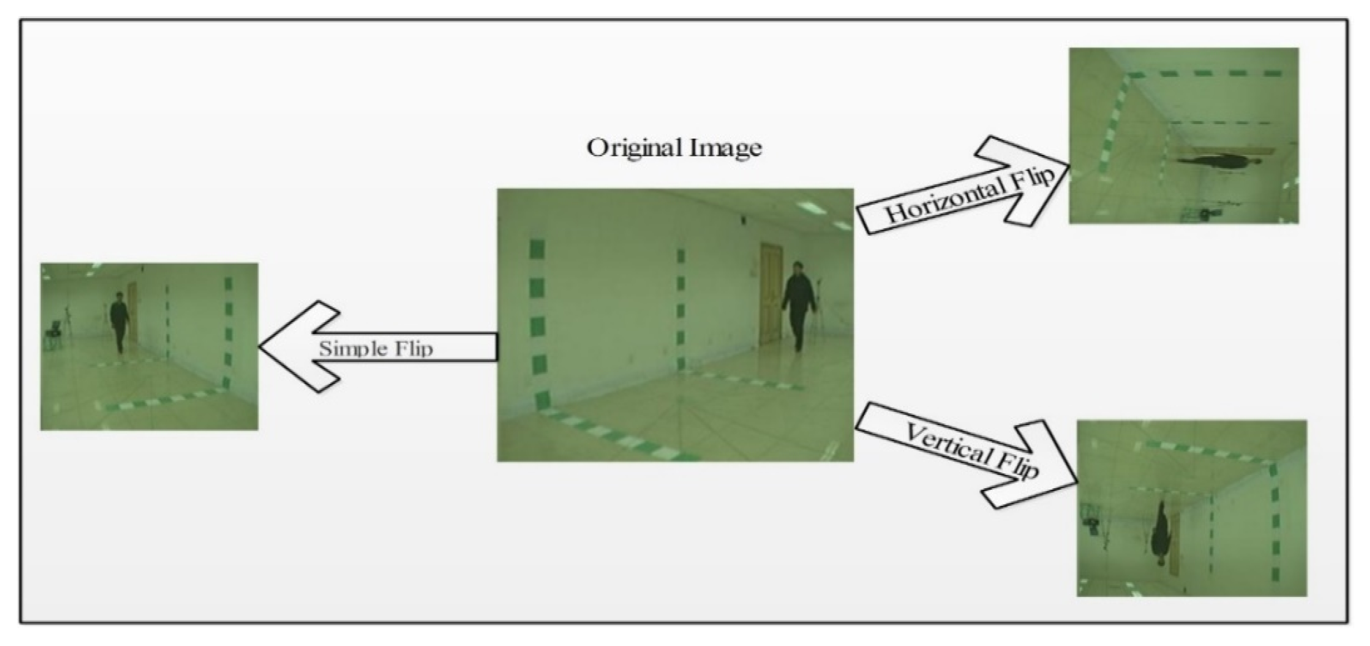
4.1. Data Augmentation
4.1.1. Left and Right Horizontal Translation
4.1.2. Up and Down Vertical Translation
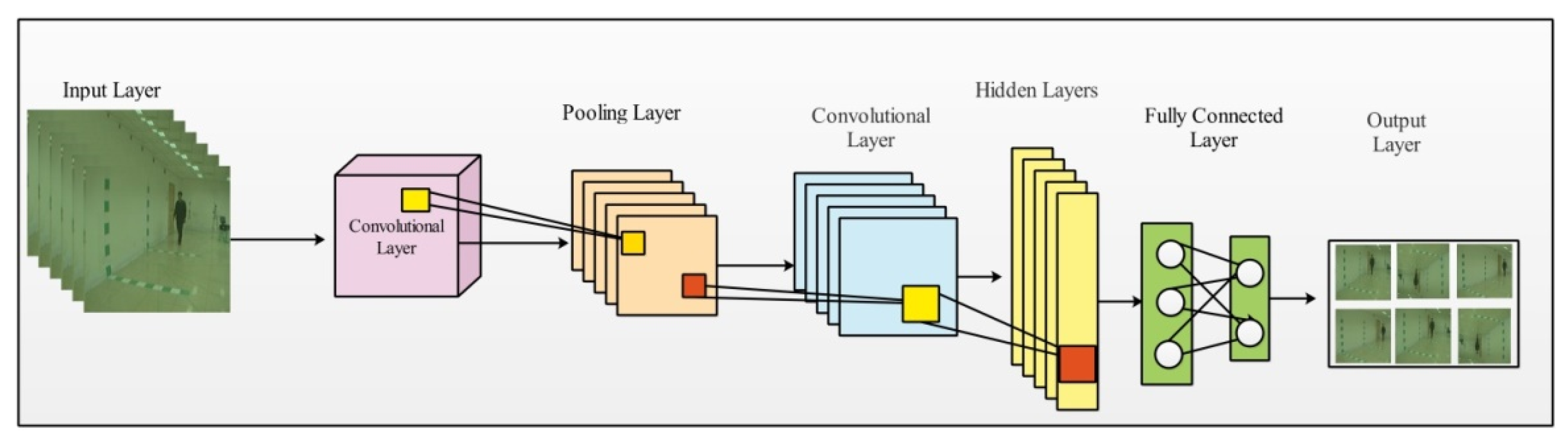
4.2. Convolutional Neural Networks (CNN)
4.2.1. Convolutional Layer
4.2.2. ReLU Layer
4.2.3. Pooling Layer
4.2.4. Batch Normalization
4.2.5. Fully Connected Layer
4.3. Transfer Learning
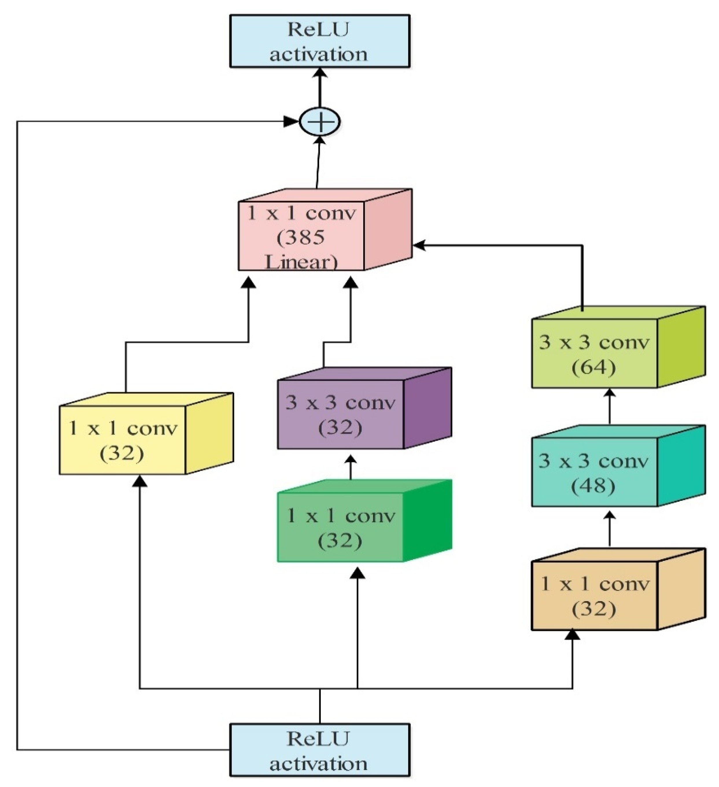
4.4. Deep Features of Modified Inception-ResNetV2
4.5. NASNet-Mobile
4.6. Novelty 1: Feature Selection
- Phase of Exploitation (circle technique of attack of prey/bubble-net)
- Phase of Exploration (searching prey)
- Define a new activation function to check the redundant features
4.6.1. Phase of Exploitation (Circle Technique of Attack of Prey/Bubble-Net)
4.6.2. Phase of Exploration (Searching Prey)
4.6.3. Phase of Final Selection
| Algorithm 1 Modified Whale Optimization for Best Features Selection |
|
4.7. Novelty 2: Feature Fusion
5. Results
5.1. Experimental Setup
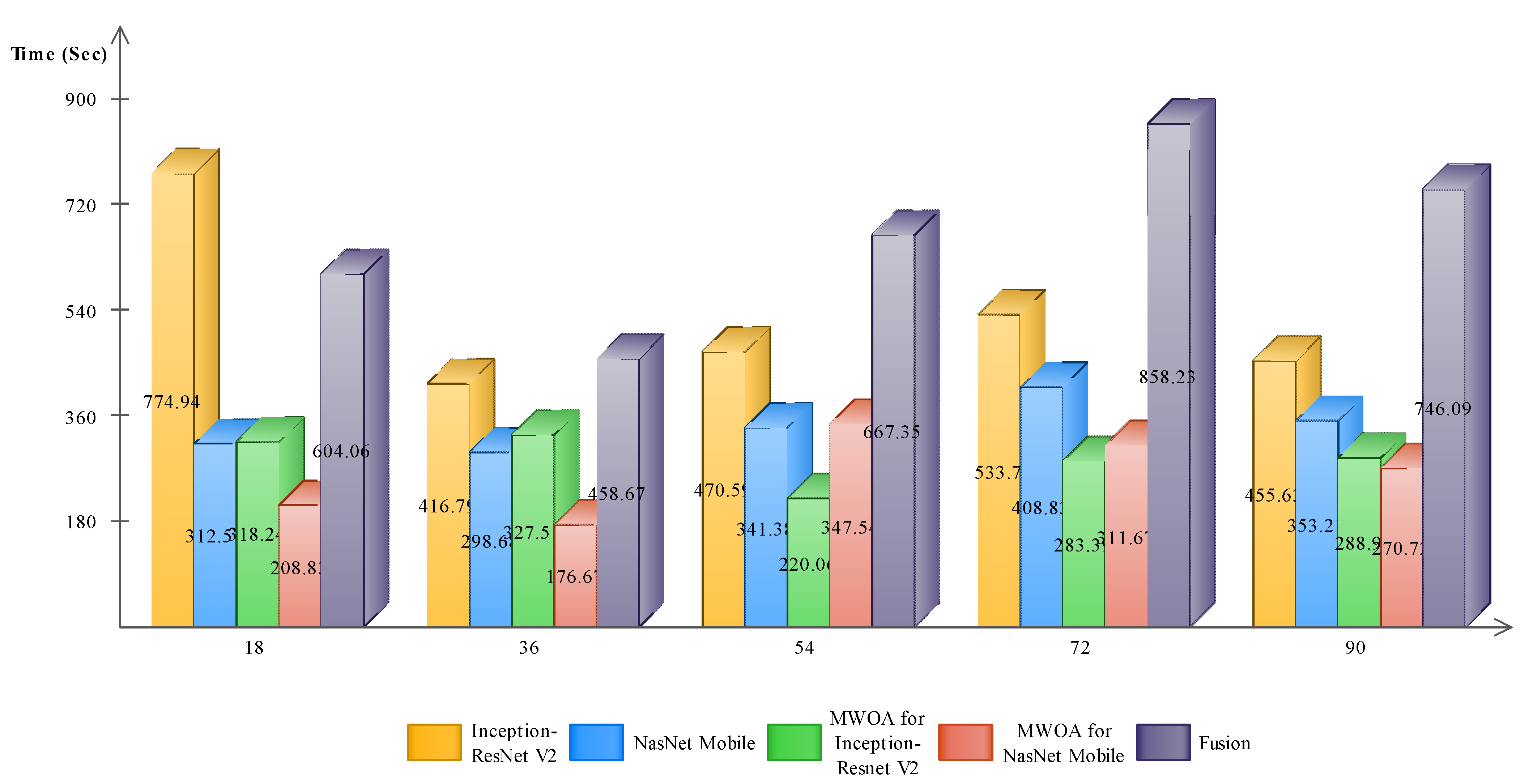
5.2. Results
6. Conclusions
- Fusion can be performed using various threshold function and then select the best of them based on the accuracy.
- Moreover, OU-MVLP, OU-LP-BAG, TUM-GAID datasets will also be considered for the experimental process.
- Adopt a two-stream approach such as optical flow based and raw images steps for the more accurate recognition accuracy.
- Extract deep features using latest deep models like Efficient Net.
Author Contributions
Funding
Data Availability Statement
Conflicts of Interest
References
- Arshad, H.; Khan, M.A.; Sharif, M.I.; Yasmin, M.; Tavares, J.M.R.; Zhang, Y.D.; Satapathy, S.C. A multilevel paradigm for deep convolutional neural network features selection with an application to human gait recognition. Expert Syst. 2020, e12541. [Google Scholar] [CrossRef]
- Manssor, S.A.; Sun, S.; Elhassan, M.A. Real-Time Human Recognition at Night via Integrated Face and Gait Recognition Technologies. Sensors 2021, 21, 4323. [Google Scholar] [CrossRef]
- Mehmood, A.; Khan, M.A.; Sharif, M.; Khan, S.A.; Shaheen, M.; Saba, T.; Riaz, N.; Ashraf, I. Prosperous human gait recognition: An end-to-end system based on pre-trained CNN features selection. Multimed. Tools Appl. 2020, 1–21. [Google Scholar] [CrossRef]
- Wang, L.; Li, Y.; Xiong, F.; Zhang, W. Gait Recognition Using Optical Motion Capture: A Decision Fusion Based Method. Sensors 2021, 21, 3496. [Google Scholar] [CrossRef]
- Khan, M.H.; Farid, M.S.; Grzegorzek, M. A non-linear view transformations model for cross-view gait recognition. Neurocomputing 2020, 402, 100–111. [Google Scholar] [CrossRef]
- Sharif, M.; Attique, M.; Tahir, M.Z.; Yasmim, M.; Saba, T.; Tanik, U.J. A machine learning method with threshold based parallel feature fusion and feature selection for automated gait recognition. J. Organ. End User Comput. (JOEUC) 2020, 32, 67–92. [Google Scholar] [CrossRef]
- Fricke, C.; Alizadeh, J.; Zakhary, N.; Woost, T.B.; Bogdan, M.; Classen, J. Evaluation of three machine learning algorithms for the automatic classification of EMG patterns in gait disorders. Front. Neurol. 2021, 12, 666458. [Google Scholar] [CrossRef]
- Gao, F.; Tian, T.; Yao, T.; Zhang, Q. Human gait recognition based on multiple feature combination and parameter optimization algorithms. Comput. Intell. Neurosci. 2021, 2021, 6693206. [Google Scholar] [CrossRef]
- Yao, T.; Gao, F.; Zhang, Q.; Ma, Y. Multi-feature gait recognition with DNN based on sEMG signals. Math. Biosci. Eng. 2021, 18, 3521–3542. [Google Scholar] [CrossRef]
- Steinmetzer, T.; Wilberg, S.; Bönninger, I.; Travieso, C.M. Analyzing gait symmetry with automatically synchronized wearable sensors in daily life. Microprocess. Microsyst. 2020, 77, 103118. [Google Scholar] [CrossRef]
- Mei, C.; Gao, F.; Li, Y. A determination method for gait event based on acceleration sensors. Sensors 2019, 19, 5499. [Google Scholar] [CrossRef] [PubMed] [Green Version]
- Luo, R.; Sun, S.; Zhang, X.; Tang, Z.; Wang, W. A low-cost end-to-end sEMG-based gait sub-phase recognition system. IEEE Trans. Neural Syst. Rehabil. Eng. 2019, 28, 267–276. [Google Scholar] [CrossRef] [PubMed]
- Liao, R.; Yu, S.; An, W.; Huang, Y. A model-based gait recognition method with body pose and human prior knowledge. Pattern Recognit. 2020, 98, 107069. [Google Scholar] [CrossRef]
- Addabbo, P.; Bernardi, M.L.; Biondi, F.; Cimitile, M.; Clemente, C.; Orlando, D. Temporal convolutional neural networks for radar micro-Doppler based gait recognition. Sensors 2021, 21, 381. [Google Scholar] [CrossRef]
- Khan, M.A.; Khan, M.A.; Ahmed, F.; Mittal, M.; Goyal, L.M.; Hemanth, D.J.; Satapathy, S.C. Gastrointestinal diseases segmentation and classification based on duo-deep architectures. Pattern Recognit. Lett. 2020, 131, 193–204. [Google Scholar] [CrossRef]
- Khan, M.A.; Kadry, S.; Parwekar, P.; Damaševičius, R.; Mehmood, A.; Khan, J.A.; Naqvi, S.R. Human gait analysis for osteoarthritis prediction: A framework of deep learning and kernel extreme learning machine. Complex Intell. Syst. 2021, 1–19. [Google Scholar] [CrossRef]
- Arshad, H.; Khan, M.A.; Sharif, M.; Yasmin, M.; Javed, M.Y. Multi-level features fusion and selection for human gait recognition: An optimized framework of Bayesian model and binomial distribution. Int. J. Mach. Learn. Cybern. 2019, 10, 3601–3618. [Google Scholar] [CrossRef]
- Farnoosh, A.; Wang, Z.; Zhu, S.; Ostadabbas, S. A Bayesian Dynamical Approach for Human Action Recognition. Sensors 2021, 21, 5613. [Google Scholar] [CrossRef]
- Shiraga, K.; Makihara, Y.; Muramatsu, D.; Echigo, T.; Yagi, Y. Geinet: View-invariant gait recognition using a convolutional neural network. In Proceedings of the 2016 International Conference on Biometrics (ICB), Halmstad, Sweden, 13–16 June 2016; pp. 1–8. [Google Scholar]
- Liu, J.; Zheng, N. Gait history image: A novel temporal template for gait recognition. In Proceedings of the 2007 IEEE International Conference on Multimedia and Expo, Beijing, China, 2–5 July 2007; pp. 663–666. [Google Scholar]
- Lv, Z.; Xing, X.; Wang, K.; Guan, D. Class energy image analysis for video sensor-based gait recognition: A review. Sensors 2015, 15, 932–964. [Google Scholar] [CrossRef] [Green Version]
- Chen, K.; Wu, S.; Li, Z. Gait Recognition Based on GFHI and Combined Hidden Markov Model. In Proceedings of the 2020 13th International Congress on Image and Signal Processing, BioMedical Engineering and Informatics (CISP-BMEI), Chengdu, China, 17–19 October 2020; pp. 287–292. [Google Scholar]
- Khan, M.A.; Akram, T.; Sharif, M.; Muhammad, N.; Javed, M.Y.; Naqvi, S.R. Improved strategy for human action recognition; experiencing a cascaded design. IET Image Process. 2019, 14, 818–829. [Google Scholar] [CrossRef]
- Sharif, A.; Khan, M.A.; Javed, K.; Gulfam, H.; Iqbal, T.; Saba, T.; Ali, H.; Nisar, W. Intelligent human action recognition: A framework of optimal features selection based on Euclidean distance and strong correlation. J. Control Eng. Appl. Inform. 2019, 21, 3–11. [Google Scholar]
- Arulananth, T.; Balaji, L.; Baskar, M.; Anbarasu, V.; Rao, K.S. PCA based dimensional data reduction and segmentation for DICOM images. Neural Process. Lett. 2020, 1–15. [Google Scholar] [CrossRef]
- Maitra, S.; Yan, J. Principle component analysis and partial least squares: Two dimension reduction techniques for regression. Appl. Multivar. Stat. Models 2008, 79, 79–90. [Google Scholar]
- Laohakiat, S.; Phimoltares, S.; Lursinsap, C. A clustering algorithm for stream data with LDA-based unsupervised localized dimension reduction. Inf. Sci. 2017, 381, 104–123. [Google Scholar] [CrossRef]
- Khan, M.A.; Sharif, M.; Javed, M.Y.; Akram, T.; Yasmin, M.; Saba, T. License number plate recognition system using entropy-based features selection approach with SVM. IET Image Process. 2018, 12, 200–209. [Google Scholar] [CrossRef]
- Siddiqui, S.; Khan, M.A.; Bashir, K.; Sharif, M.; Azam, F.; Javed, M.Y. Human action recognition: A construction of codebook by discriminative features selection approach. Int. J. Appl. Pattern Recognit. 2018, 5, 206–228. [Google Scholar] [CrossRef]
- Khan, M.A.; Arshad, H.; Nisar, W.; Javed, M.Y.; Sharif, M. An Integrated Design of Fuzzy C-Means and NCA-Based Multi-properties Feature Reduction for Brain Tumor Recognition. In Signal and Image Processing Techniques for the Development of Intelligent Healthcare Systems; Springer: Berlin/Heidelberg, Germany, 2021; pp. 1–28. [Google Scholar]
- Jiang, X.; Zhang, Y.; Yang, Q.; Deng, B.; Wang, H. Millimeter-Wave Array Radar-Based Human Gait Recognition Using Multi-Channel Three-Dimensional Convolutional Neural Network. Sensors 2020, 20, 5466. [Google Scholar] [CrossRef]
- Khan, M.A.; Zhang, Y.-D.; Khan, S.A.; Attique, M.; Rehman, A.; Seo, S. A resource conscious human action recognition framework using 26-layered deep convolutional neural network. Multimed. Tools Appl. 2020, 1–23. [Google Scholar] [CrossRef]
- Lu, S.; Wang, S.-H.; Zhang, Y.-D. Detection of abnormal brain in MRI via improved AlexNet and ELM optimized by chaotic bat algorithm. Neural Comput. Appl. 2020, 33, 10799–10811. [Google Scholar] [CrossRef]
- Liu, S.; Wang, X.; Zhao, L.; Li, B.; Hu, W.; Yu, J.; Zhang, Y. 3DCANN: A Spatio-Temporal Convolution Attention Neural Network for EEG Emotion Recognition. IEEE J. Biomed. Health Inform. 2021. [Google Scholar] [CrossRef]
- Wang, S.; Celebi, M.E.; Zhang, Y.-D.; Yu, X.; Lu, S.; Yao, X.; Zhou, Q.; Miguel, M.-G.; Tian, Y.; Gorriz, J.M. Advances in Data Preprocessing for Biomedical Data Fusion: An Overview of the Methods, Challenges, and Prospects. Inf. Fusion 2021, 76, 376–421. [Google Scholar] [CrossRef]
- Liu, X.; Song, L.; Liu, S.; Zhang, Y. A review of deep-learning-based medical image segmentation methods. Sustainability 2021, 13, 1224. [Google Scholar] [CrossRef]
- Zhang, Y.-D.; Dong, Z.; Wang, S.-H.; Yu, X.; Yao, X.; Zhou, Q.; Hu, H.; Li, M.; Jiménez-Mesa, C.; Ramirez, J. Advances in multimodal data fusion in neuroimaging: Overview, challenges, and novel orientation. Inf. Fusion 2020, 64, 149–187. [Google Scholar] [CrossRef]
- Wang, X.; Zhang, J.; Yan, W.Q. Gait recognition using multichannel convolution neural networks. Neural Comput. Appl. 2019, 32, 14275–14285. [Google Scholar] [CrossRef]
- Khan, M.A.; Zhang, Y.-D.; Alhusseni, M.; Kadry, S.; Wang, S.-H.; Saba, T.; Iqbal, T. A Fused Heterogeneous Deep Neural Network and Robust Feature Selection Framework for Human Actions Recognition. Arab. J. Sci. Eng. 2021, 1–16. [Google Scholar] [CrossRef]
- Hussain, N.; Khan, M.A.; Kadry, S.; Tariq, U.; Mostafa, R.R.; Choi, J.-I.; Nam, Y. Intelligent Deep Learning and Improved Whale Optimization Algorithm Based Framework for Object Recognition. Hum. Cent. Comput. Inf. Sci. 2021, 11, 34. [Google Scholar]
- Hussain, N.; Khan, M.A.; Tariq, U.; Kadry, S.; Yar, M.A.E.; Mostafa, A.M.; Alnuaim, A.A.; Ahmad, S. Multiclass Cucumber Leaf Diseases Recognition Using Best Feature Selection. Comput. Mater. Contin. 2022, 70, 3281–3294. [Google Scholar] [CrossRef]
- Kiran, S.; Khan, M.A.; Javed, M.Y.; Alhaisoni, M.; Tariq, U.; Nam, Y.; Damaševičius, R.; Sharif, M. Multi-Layered Deep Learning Features Fusion for Human Action Recognition. Comput. Mater. Contin. 2021, 69, 4061–4075. [Google Scholar] [CrossRef]
- Majid, A.; Khan, M.A.; Nam, Y.; Tariq, U.; Roy, S.; Mostafa, R.R.; Sakr, R.H. COVID19 classification using CT images via ensembles of deep learning models. Comput. Mater. Contin. 2021, 69, 319–337. [Google Scholar] [CrossRef]
- Khan, M.A.; Alhaisoni, M.; Armghan, A.; Alenezi, F.; Tariq, U.; Nam, Y.; Akram, T. Video Analytics Framework for Human Action Recognition. CMC-Comput. Mater. Contin. 2021, 68, 3841–3859. [Google Scholar] [CrossRef]
- Afza, F.; Khan, M.A.; Sharif, M.; Kadry, S.; Manogaran, G.; Saba, T.; Ashraf, I.; Damaševičius, R. A framework of human action recognition using length control features fusion and weighted entropy-variances based feature selection. Image Vis. Comput. 2021, 106, 104090. [Google Scholar] [CrossRef]
- Hussain, N.; Khan, M.A.; Sharif, M.; Khan, S.A.; Albesher, A.A.; Saba, T.; Armaghan, A. A deep neural network and classical features based scheme for objects recognition: An application for machine inspection. Multimed. Tools Appl. 2020, 1–23. [Google Scholar] [CrossRef]
- Gul, S.; Malik, M.I.; Khan, G.M.; Shafait, F. Multi-view gait recognition system using spatio-temporal features and deep learning. Expert Syst. Appl. 2021, 179, 115057. [Google Scholar] [CrossRef]
- Davarzani, S.; Saucier, D.; Peranich, P.; Carroll, W.; Turner, A.; Parker, E.; Middleton, C.; Nguyen, P.; Robertson, P.; Smith, B. Closing the wearable gap—Part VI: Human gait recognition using deep learning methodologies. Electronics 2020, 9, 796. [Google Scholar] [CrossRef]
- Anusha, R.; Jaidhar, C. Clothing invariant human gait recognition using modified local optimal oriented pattern binary descriptor. Multimed. Tools Appl. 2020, 79, 2873–2896. [Google Scholar] [CrossRef]
- Jun, K.; Lee, D.-W.; Lee, K.; Lee, S.; Kim, M.S. Feature extraction using an RNN autoencoder for skeleton-based abnormal gait recognition. IEEE Access 2020, 8, 19196–19207. [Google Scholar] [CrossRef]
- Anusha, R.; Jaidhar, C. Human gait recognition based on histogram of oriented gradients and Haralick texture descriptor. Multimed. Tools Appl. 2020, 79, 8213–8234. [Google Scholar] [CrossRef]
- Elharrouss, O.; Almaadeed, N.; Al-Maadeed, S.; Bouridane, A. Gait recognition for person re-identification. J. Supercomput. 2020, 77, 3653–3672. [Google Scholar] [CrossRef]
- Nithyakani, P.; Shanthini, A.; Ponsam, G. Human gait recognition using deep convolutional neural network. In Proceedings of the 2019 3rd International Conference on Computing and Communications Technologies (ICCCT), Chennai, India, 21–22 February 2019; pp. 208–211. [Google Scholar]
- Hasan, M.M.; Mustafa, H.A. Multi-level feature fusion for robust pose-based gait recognition using RNN. Int. J. Comput. Sci. Inf. Secur. (IJCSIS) 2020, 18, 20–31. [Google Scholar]
- Bai, X.; Hui, Y.; Wang, L.; Zhou, F. Radar-based human gait recognition using dual-channel deep convolutional neural network. IEEE Trans. Geosci. Remote Sens. 2019, 57, 9767–9778. [Google Scholar] [CrossRef]
- Zheng, S.; Zhang, J.; Huang, K.; He, R.; Tan, T. Robust view transformation model for gait recognition. In Proceedings of the 2011 18th IEEE International Conference on Image Processing, Brussels, Belgium, 11–14 September 2011; pp. 2073–2076. [Google Scholar]
- Chao, H.; He, Y.; Zhang, J.; Feng, J. Gaitset: Regarding gait as a set for cross-view gait recognition. In Proceedings of the AAAI Conference on Artificial Intelligence, Honolulu, HI, USA, 27 January 27–1 February 2019; pp. 8126–8133. [Google Scholar]
- Lavin, A.; Gray, S. Fast algorithms for convolutional neural networks. In Proceedings of the IEEE Conference on Computer Vision and Pattern Recognition, Las Vegas, NV, USA, 27–30 June 2016; pp. 4013–4021. [Google Scholar]
- Rashid, M.; Khan, M.A.; Alhaisoni, M.; Wang, S.-H.; Naqvi, S.R.; Rehman, A.; Saba, T. A sustainable deep learning framework for object recognition using multi-layers deep features fusion and selection. Sustainability 2020, 12, 5037. [Google Scholar] [CrossRef]
- Zou, Q.; Wang, Y.; Wang, Q.; Zhao, Y.; Li, Q. Deep learning-based gait recognition using smartphones in the wild. IEEE Trans. Inf. Forensics Secur. 2020, 15, 3197–3212. [Google Scholar] [CrossRef] [Green Version]
- Vedaldi, A.; Lenc, K. Matconvnet: Convolutional neural networks for matlab. In Proceedings of the 23rd ACM International Conference on Multimedia, Brisbane, Australia, 26–30 October 2015; pp. 689–692. [Google Scholar]
- Mafarja, M.; Mirjalili, S. Whale optimization approaches for wrapper feature selection. Appl. Soft Comput. 2018, 62, 441–453. [Google Scholar] [CrossRef]
- Adeel, A.; Khan, M.A.; Akram, T.; Sharif, A.; Yasmin, M.; Saba, T.; Javed, K. Entropy-controlled deep features selection framework for grape leaf diseases recognition. Expert Syst. 2020. [Google Scholar] [CrossRef]
- Khan, M.A.; Sharif, M.I.; Raza, M.; Anjum, A.; Saba, T.; Shad, S.A. Skin lesion segmentation and classification: A unified framework of deep neural network features fusion and selection. Expert Syst. 2019, e12497. [Google Scholar] [CrossRef]
- Yang, J.; Yang, J.-y.; Zhang, D.; Lu, J.-F. Feature fusion: Parallel strategy vs. serial strategy. Pattern Recognit. 2003, 36, 1369–1381. [Google Scholar] [CrossRef]
- Wu, Z.; Huang, Y.; Wang, L.; Wang, X.; Tan, T. A comprehensive study on cross-view gait based human identification with deep cnns. IEEE Trans. Pattern Anal. Mach. Intell. 2016, 39, 209–226. [Google Scholar] [CrossRef]


| Epochs | 100 |
| Learning Rate | 0.05 |
| Mini-Batch Size | 64 |
| Learning Method | SGD |
| WeightLearnRateFactor | 20 |
| LearnRateDropPeriod | 6 |
| Classifier | Angles | Performance Measures | |||||||
|---|---|---|---|---|---|---|---|---|---|
| Cubic (SVM) | 18 | 36 | 54 | 72 | 90 | Recall Rate (%) | F1-Score | Accuracy (%) | Time (s) |
| ❖ | 88.73 | 88.80 | 88.8 | 134.74 | |||||
| ❖ | 84.7 | 84.64 | 84.6 | 219.09 | |||||
| ❖ | 85.1 | 85.1 | 85.1 | 234.95 | |||||
| ❖ | 76.5 | 76.44 | 76.4 | 238.18 | |||||
| ❖ | 79 | 79.02 | 78.9 | 207.65 | |||||
| Quadratic (QSVM) | ❖ | 87 | 87.12 | 87.1 | 122.2 | ||||
| ❖ | 83.5 | 83.44 | 83.4 | 205.2 | |||||
| ❖ | 83.1 | 83.06 | 83.0 | 213.94 | |||||
| ❖ | 75.9 | 75.86 | 75.8 | 222.8 | |||||
| ❖ | 78.5 | 78.72 | 78.4 | 197.3 | |||||
| Medium Gaussian (MGSVM) | ❖ | 81.16 | 81.44 | 81.3 | 150.09 | ||||
| ❖ | 78.2 | 78.14 | 78.1 | 261.9 | |||||
| ❖ | 77.23 | 77.47 | 77.2 | 269.01 | |||||
| ❖ | 72.56 | 72.57 | 72.5 | 268.82 | |||||
| ❖ | 75.5 | 76.45 | 75.6 | 246.48 | |||||
| Subspace Discriminant (SD) | ❖ | 81.16 | 81.44 | 81.3 | 150.09 | ||||
| ❖ | 78.2 | 78.14 | 78.1 | 261.9 | |||||
| ❖ | 77.23 | 77.47 | 77.2 | 269.01 | |||||
| ❖ | 72.56 | 72.57 | 72.5 | 268.82 | |||||
| ❖ | 75.5 | 76.45 | 75.6 | 246.48 | |||||
| Classifier | Angles | Performance Measures | |||||||
|---|---|---|---|---|---|---|---|---|---|
| Cubic (SVM) | 18 | 36 | 54 | 72 | 90 | Recall Rate (%) | F1-Score | Accuracy (%) | Time (s) |
| ❖ | 86.93 | 86.97 | 87.0 | 140.32 | |||||
| ❖ | 83.7 | 83.66 | 83.6 | 752.26 | |||||
| ❖ | 80.43 | 80.39 | 80.4 | 165.36 | |||||
| ❖ | 72.36 | 72.34 | 72.3 | 174.19 | |||||
| ❖ | 73.03 | 73.04 | 73.0 | 161.92 | |||||
| Quadratic (SVM) | ❖ | 85.2 | 85.29 | 85.3 | 136.44 | ||||
| ❖ | 81.56 | 81.47 | 81.4 | 147.41 | |||||
| ❖ | 79.26 | 79.20 | 79.2 | 159.89 | |||||
| ❖ | 71.43 | 71.41 | 71.4 | 162.87 | |||||
| ❖ | 73.23 | 73.27 | 73.2 | 152.06 | |||||
| Medium Gaussian (SVM) | ❖ | 82.56 | 82.77 | 82.6 | 179.14 | ||||
| ❖ | 78.96 | 78.94 | 78.9 | 171.86 | |||||
| ❖ | 74.83 | 74.84 | 74.7 | 189.51 | |||||
| ❖ | 69.6 | 69.62 | 69.5 | 195.77 | |||||
| ❖ | 70.1 | 70.77 | 70.2 | 188.1 | |||||
| Subspace Discriminant | ❖ | 81.8 | 81.86 | 81.9 | 244.1 | ||||
| ❖ | 75.3 | 75.24 | 75.2 | 231.83 | |||||
| ❖ | 74.7 | 74.59 | 74.5 | 246.87 | |||||
| ❖ | 69.23 | 69.17 | 69.1 | 245.52 | |||||
| ❖ | 70.53 | 70.59 | 70.4 | 358.05 | |||||
| Classifier | Angles | Performance Measures | |||||||
|---|---|---|---|---|---|---|---|---|---|
| Cubic (SVM) | 18 | 36 | 54 | 72 | 90 | Recall Rate (%) | F1-Score | Accuracy (%) | Time (s) |
| ❖ | 95.56 | 95.58 | 95.6 | 774.94 | |||||
| ❖ | 92.6 | 92.62 | 92.6 | 416.79 | |||||
| ❖ | 92.7 | 92.7 | 92.7 | 470.59 | |||||
| ❖ | 86.16 | 86.16 | 86.2 | 533.7 | |||||
| ❖ | 87.76 | 87.74 | 87.7 | 455.63 | |||||
| Quadratic (SVM) | ❖ | 93.73 | 93.74 | 93.7 | 613.87 | ||||
| ❖ | 89.86 | 89.88 | 89.9 | 405.87 | |||||
| ❖ | 90.63 | 90.61 | 90.6 | 466.01 | |||||
| ❖ | 83.46 | 83.42 | 83.5 | 546.39 | |||||
| ❖ | 84.23 | 84.21 | 84.2 | 453.3 | |||||
| Medium Gaussian (SVM) | ❖ | 88.93 | 89.09 | 88.9 | 877.84 | ||||
| ❖ | 85.56 | 85.59 | 85.6 | 553.11 | |||||
| ❖ | 86.26 | 86.30 | 86.3 | 617.03 | |||||
| ❖ | 79.93 | 79.89 | 79.9 | 645.77 | |||||
| ❖ | 81.23 | 81.21 | 81.2 | 553.25 | |||||
| Subspace Discriminant | ❖ | 89.1 | 89.14 | 89.1 | 1101.9 | ||||
| ❖ | 86.4 | 86.4 | 86.4 | 814.27 | |||||
| ❖ | 86.36 | 86.36 | 86.4 | 696.59 | |||||
| ❖ | 79.56 | 79.49 | 79.6 | 708.82 | |||||
| ❖ | 81.83 | 81.77 | 81.8 | 860.23 | |||||
| Classifier | Angles | Performance Measures | |||||||
|---|---|---|---|---|---|---|---|---|---|
| Cubic (SVM) | 18 | 36 | 54 | 72 | 90 | Recall Rate (%) | F1-Score | Accuracy (%) | Time (s) |
| ❖ | 94.43 | 94.46 | 94.4 | 312.57 | |||||
| ❖ | 92.13 | 92.13 | 92.1 | 298.68 | |||||
| ❖ | 90.9 | 90.9 | 90.9 | 341.38 | |||||
| ❖ | 83.5 | 83.5 | 83.5 | 408.83 | |||||
| ❖ | 84.8 | 84.78 | 84.8 | 353.21 | |||||
| Quadratic (SVM) | ❖ | 92.43 | 92.43 | 92.4 | 318.57 | ||||
| ❖ | 89.76 | 89.76 | 89.7 | 311.06 | |||||
| ❖ | 87.83 | 87.83 | 87.8 | 341.79 | |||||
| ❖ | 80.8 | 80.74 | 80.8 | 394.58 | |||||
| ❖ | 81.73 | 81.71 | 81.7 | 336.79 | |||||
| Medium Gaussian (SVM) | ❖ | 90.65 | 90.70 | 90.6 | 408.38 | ||||
| ❖ | 87.2 | 87.21 | 87.2 | 384.16 | |||||
| ❖ | 84.3 | 84.3 | 84.1 | 424.26 | |||||
| ❖ | 77.6 | 77.6 | 77.6 | 484.31 | |||||
| ❖ | 78.83 | 78.86 | 78.9 | 408.07 | |||||
| Subspace Discriminant | ❖ | 82.9 | 82.92 | 82.9 | 372.4 | ||||
| ❖ | 80.13 | 80.14 | 80.2 | 461.67 | |||||
| ❖ | 79.36 | 79.34 | 79.4 | 392.91 | |||||
| ❖ | 77.63 | 75.54 | 73.6 | 367.88 | |||||
| ❖ | 75.46 | 75.42 | 75.5 | 345.69 | |||||
| Classifier | Angles | Performance Measures | |||||||
|---|---|---|---|---|---|---|---|---|---|
| Cubic (SVM) | 18 | 36 | 54 | 72 | 90 | Recall Rate (%) | F1- Score | Accuracy (%) | Time (s) |
| ❖ | 95.16 | 95.16 | 95.2 | 318.24 | |||||
| ❖ | 92.53 | 92.53 | 92.5 | 327.51 | |||||
| ❖ | 91.36 | 91.36 | 91.4 | 220.06 | |||||
| ❖ | 85.3 | 85.3 | 85.3 | 283.39 | |||||
| ❖ | 86.33 | 86.31 | 86.4 | 288.9 | |||||
| Quadratic (SVM) | ❖ | 92.93 | 92.96 | 92.9 | 319 | ||||
| ❖ | 89.43 | 89.5 | 89.5 | 327.05 | |||||
| ❖ | 88.9 | 88.88 | 88.9 | 213.95 | |||||
| ❖ | 83.06 | 83.02 | 83.1 | 273.6 | |||||
| ❖ | 83.36 | 83.32 | 83.4 | 284.15 | |||||
| Medium Gaussian (SVM) | ❖ | 88.8 | 88.96 | 88.8 | 419.4 | ||||
| ❖ | 86 | 86.01 | 86.0 | 416.31 | |||||
| ❖ | 85.1 | 85.14 | 85.1 | 251.64 | |||||
| ❖ | 80 | 79.96 | 80.0 | 309.81 | |||||
| ❖ | 80.73 | 80.73 | 80.7 | 350.5 | |||||
| Subspace Discriminant | ❖ | 85.23 | 85.29 | 85.2 | 435.82 | ||||
| ❖ | 83.63 | 83.59 | 83.6 | 380.47 | |||||
| ❖ | 77.66 | 77.66 | 77.7 | 153.97 | |||||
| ❖ | 75.7 | 75.59 | 75.7 | 221.19 | |||||
| ❖ | 78.83 | 78.77 | 78.8 | 331.38 | |||||
| Classifier | Angles | Performance Measures | |||||||
|---|---|---|---|---|---|---|---|---|---|
| Cubic (SVM) | 18 | 36 | 54 | 72 | 90 | Recall Rate (%) | F1- Score | Accuracy (%) | Time (s) |
| ❖ | 94.1 | 94.1 | 94.1 | 208.83 | |||||
| ❖ | 91.33 | 91.33 | 91.3 | 176.67 | |||||
| ❖ | 90.7 | 90.68 | 90.7 | 347.54 | |||||
| ❖ | 82.66 | 82.69 | 82.7 | 311.67 | |||||
| ❖ | 83.96 | 83.98 | 84.0 | 270.72 | |||||
| Quadratic (SVM) | ❖ | 91.73 | 91.76 | 91.7 | 213.91 | ||||
| ❖ | 88.23 | 88.24 | 88.2 | 184.07 | |||||
| ❖ | 87.83 | 87.81 | 87.8 | 341.09 | |||||
| ❖ | 79.36 | 79.32 | 79.4 | 304.87 | |||||
| ❖ | 80.83 | 80.83 | 80.8 | 254.24 | |||||
| Medium Gaussian (SVM) | ❖ | 90 | 90.11 | 90.0 | 257.75 | ||||
| ❖ | 86.06 | 86.09 | 86.1 | 198.9 | |||||
| ❖ | 83.6 | 83.67 | 83.8 | 415.73 | |||||
| ❖ | 77.1 | 77.1 | 77.1 | 369.89 | |||||
| ❖ | 77.83 | 77.8 | 77.8 | 294.81 | |||||
| Subspace Discriminant | ❖ | 78.6 | 78.62 | 78.6 | 193.54 | ||||
| ❖ | 73.66 | 73.66 | 73.7 | 146.74 | |||||
| ❖ | 78.2 | 78.2 | 78.2 | 357.09 | |||||
| ❖ | 71.5 | 75.42 | 71.5 | 258.36 | |||||
| ❖ | 72.13 | 72.16 | 72.2 | 205.73 | |||||
| Classifier | Angles | Performance Measures | |||||||
|---|---|---|---|---|---|---|---|---|---|
| Cubic (SVM) | 18 | 36 | 54 | 72 | 90 | Recall Rate (%) | F1- Score | Accuracy (%) | Time (s) |
| ❖ | 97.23 | 97.24 | 97.3 | 604.06 | |||||
| ❖ | 96.03 | 95.99 | 96.0 | 458.67 | |||||
| ❖ | 95.3 | 95.28 | 95.3 | 667.35 | |||||
| ❖ | 86.63 | 86.61 | 86.6 | 858.23 | |||||
| ❖ | 86.43 | 88.06 | 89.8 | 746.09 | |||||
| Quadratic (SVM) | ❖ | 95.96 | 95.98 | 96 | 565.47 | ||||
| ❖ | 95.06 | 95.08 | 95.1 | 417.4 | |||||
| ❖ | 93.4 | 93.44 | 93.4 | 631.4 | |||||
| ❖ | 84.1 | 84.04 | 84.1 | 841.61 | |||||
| ❖ | 87.36 | 87.34 | 87.4 | 689.05 | |||||
| Medium Gaussian (SVM) | ❖ | 94.03 | 94.11 | 94.1 | 882.62 | ||||
| ❖ | 93.03 | 93.03 | 93 | 628.42 | |||||
| ❖ | 91.5 | 91.53 | 91.5 | 867.96 | |||||
| ❖ | 81.86 | 81.80 | 81.9 | 1089.3 | |||||
| ❖ | 85.73 | 85.73 | 85.7 | 927.9 | |||||
| Subspace Discriminant | ❖ | 94.66 | 94.68 | 94.7 | 719.94 | ||||
| ❖ | 93.16 | 93.16 | 93.1 | 650.3 | |||||
| ❖ | 92.23 | 92.24 | 92.2 | 1356.5 | |||||
| ❖ | 82.8 | 82.74 | 82.8 | 1411.7 | |||||
| ❖ | 87.26 | 87.23 | 87.2 | 1504.8 | |||||
| Min (%) | Avg (%) | Max (%) | CI | |||
|---|---|---|---|---|---|---|
| 0 | 71.4 | 72.3 | 73.2 | 0.90 | 0.6363 | 72.3 ± 1.247 (±1.73%) |
| 18 | 96.1 | 96.70 | 97.3 | 0.60 | 0.4242 | 96.7 ± 0.832 (±0.86%) |
| 36 | 95.3 | 95.65 | 96.0 | 0.35 | 0.2474 | 95.65 ± 0.485 (±0.51%) |
| 54 | 93.8 | 94.55 | 95.3 | 0.75 | 0.5303 | 94.55 ± 1.039 (±1.10%) |
| 72 | 85.2 | 85.90 | 86.6 | 0.70 | 0.4949 | 85.9 ± 0.97 (±1.13%) |
| 90 | 88.5 | 89.15 | 89.8 | 0.65 | 0.4596 | 89.15 ± 0.901 (±1.10%) |
| 108 | 93.1 | 93.85 | 94.6 | 0.75 | 0.5303 | 93.85 ±1.039 (±1.11%) |
| 126 | 91.8 | 92.8 | 93.8 | 1.0 | 0.7071 | 92.8 ± 1.386 (±1.49%) |
| 144 | 78.6 | 80.0 | 81.4 | 1.4 | 0.9899 | 80 ± 1.94 (±2.43%) |
| 162 | 88.4 | 89.6 | 90.8 | 1.2 | 0.8485 | 89.6 ± 1.663 (±1.86%) |
| 180 | 77.6 | 78.3 | 80.3 | 0.75 | 0.5303 | 78.35 ± 1.039 (±1.33%) |
| Reference | Angle | Mean Accuracy (%) |
|---|---|---|
| Chao et al. [57], 2019 | All 11 angles with three variations | 84.20 |
| Wu et al. [66], 2016 | All 11 angles with three variations | 73.49 |
| Mehmood et al. [3], 2020 | 18, 36, 54 | 94.26 |
| Proposed | All 11 angles with three variations | 89.00 |
Publisher’s Note: MDPI stays neutral with regard to jurisdictional claims in published maps and institutional affiliations. |
© 2021 by the authors. Licensee MDPI, Basel, Switzerland. This article is an open access article distributed under the terms and conditions of the Creative Commons Attribution (CC BY) license (https://creativecommons.org/licenses/by/4.0/).
Share and Cite
Saleem, F.; Khan, M.A.; Alhaisoni, M.; Tariq, U.; Armghan, A.; Alenezi, F.; Choi, J.-I.; Kadry, S. Human Gait Recognition: A Single Stream Optimal Deep Learning Features Fusion. Sensors 2021, 21, 7584. https://doi.org/10.3390/s21227584
Saleem F, Khan MA, Alhaisoni M, Tariq U, Armghan A, Alenezi F, Choi J-I, Kadry S. Human Gait Recognition: A Single Stream Optimal Deep Learning Features Fusion. Sensors. 2021; 21(22):7584. https://doi.org/10.3390/s21227584
Chicago/Turabian StyleSaleem, Faizan, Muhammad Attique Khan, Majed Alhaisoni, Usman Tariq, Ammar Armghan, Fayadh Alenezi, Jung-In Choi, and Seifedine Kadry. 2021. "Human Gait Recognition: A Single Stream Optimal Deep Learning Features Fusion" Sensors 21, no. 22: 7584. https://doi.org/10.3390/s21227584
APA StyleSaleem, F., Khan, M. A., Alhaisoni, M., Tariq, U., Armghan, A., Alenezi, F., Choi, J.-I., & Kadry, S. (2021). Human Gait Recognition: A Single Stream Optimal Deep Learning Features Fusion. Sensors, 21(22), 7584. https://doi.org/10.3390/s21227584