
An Efficient Methodology for Brain MRI Classification Based on DWT and Convolutional Neural Network

 , ,
, ,  and
and
Abstract
:1. Introduction
2. Related Work
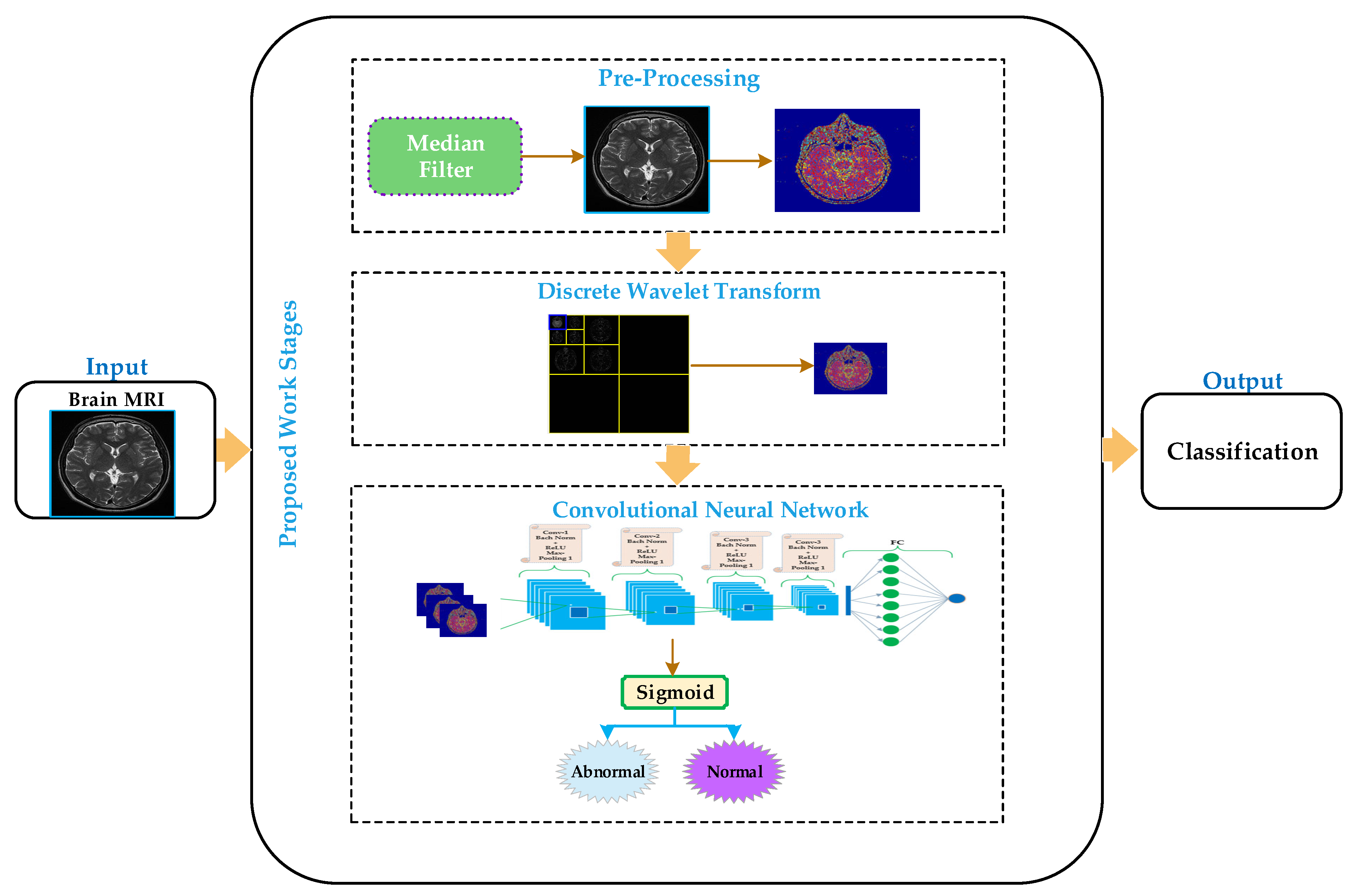
3. Proposed Methodology
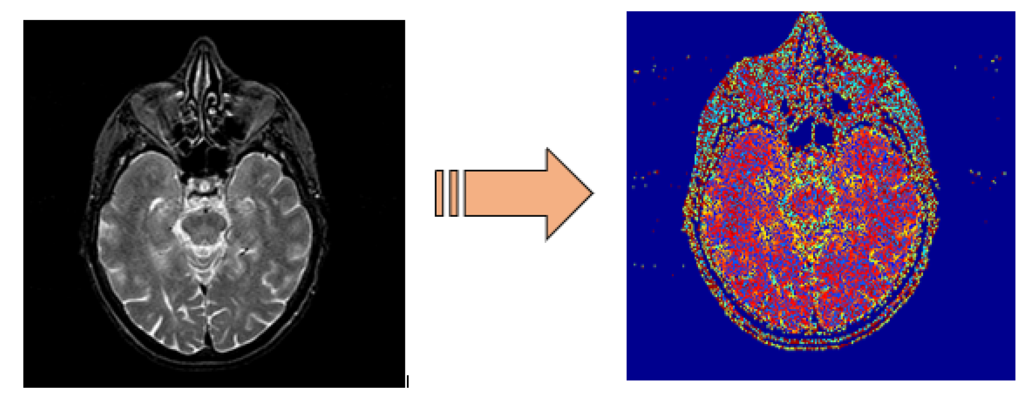
3.1. Preprocessing
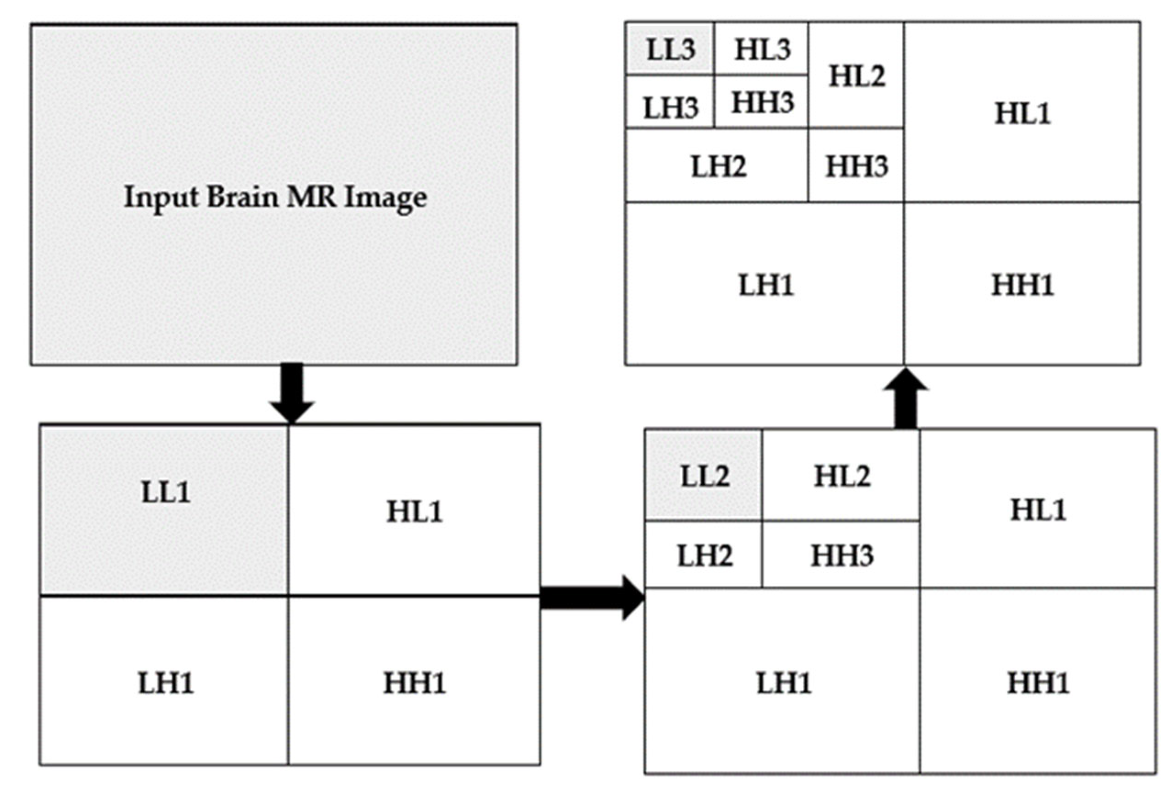
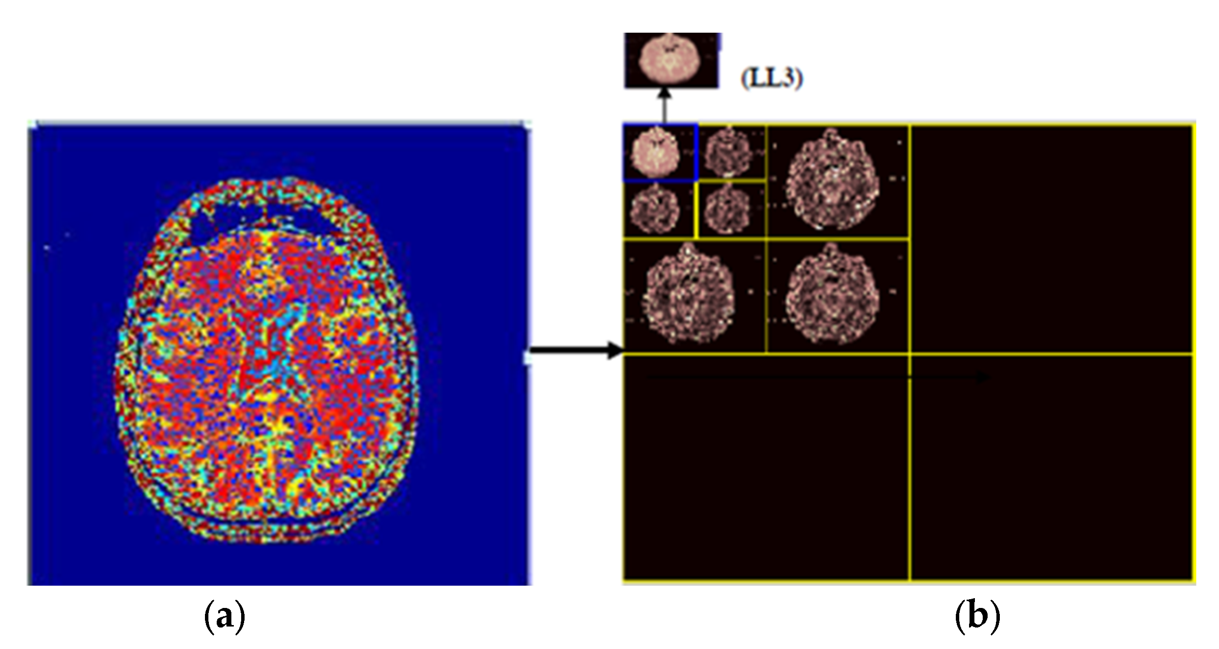
3.2. Discrete Wavelet Transform
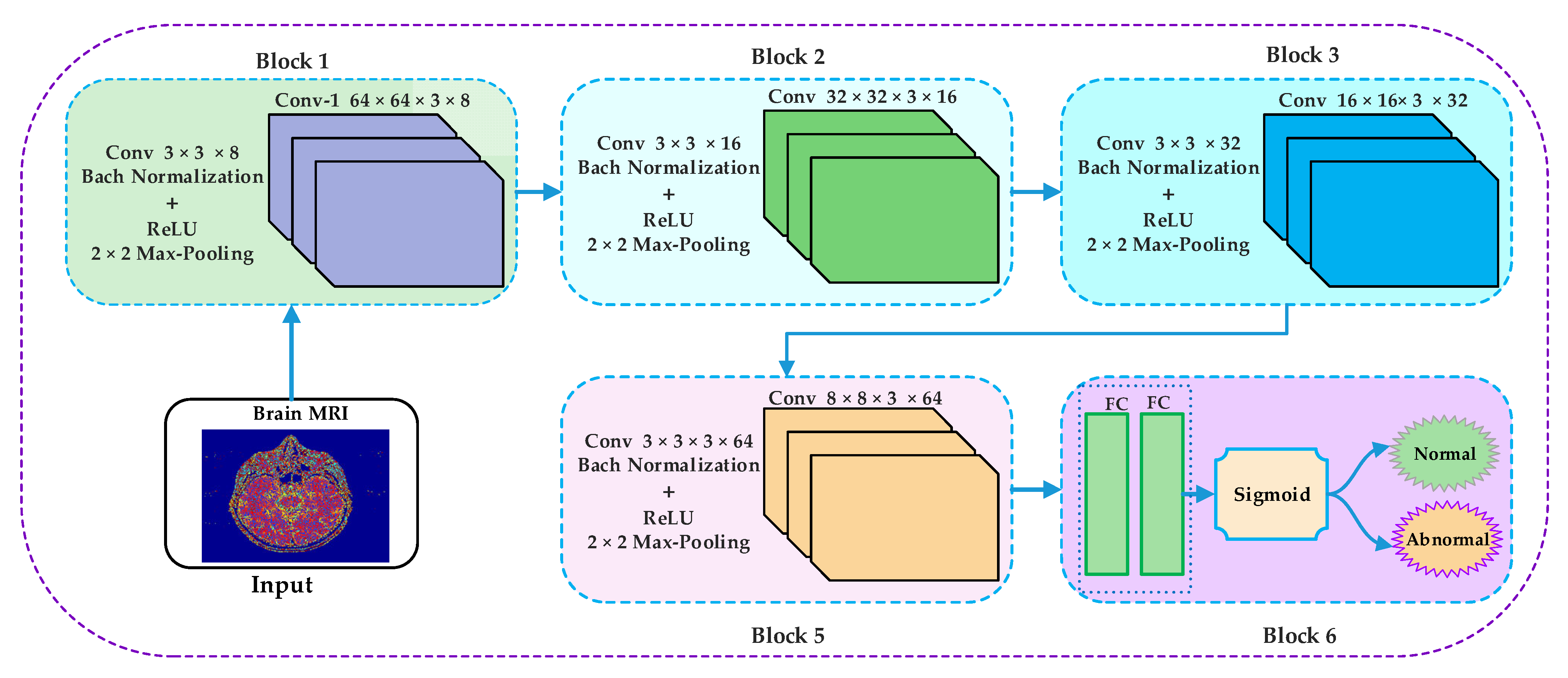
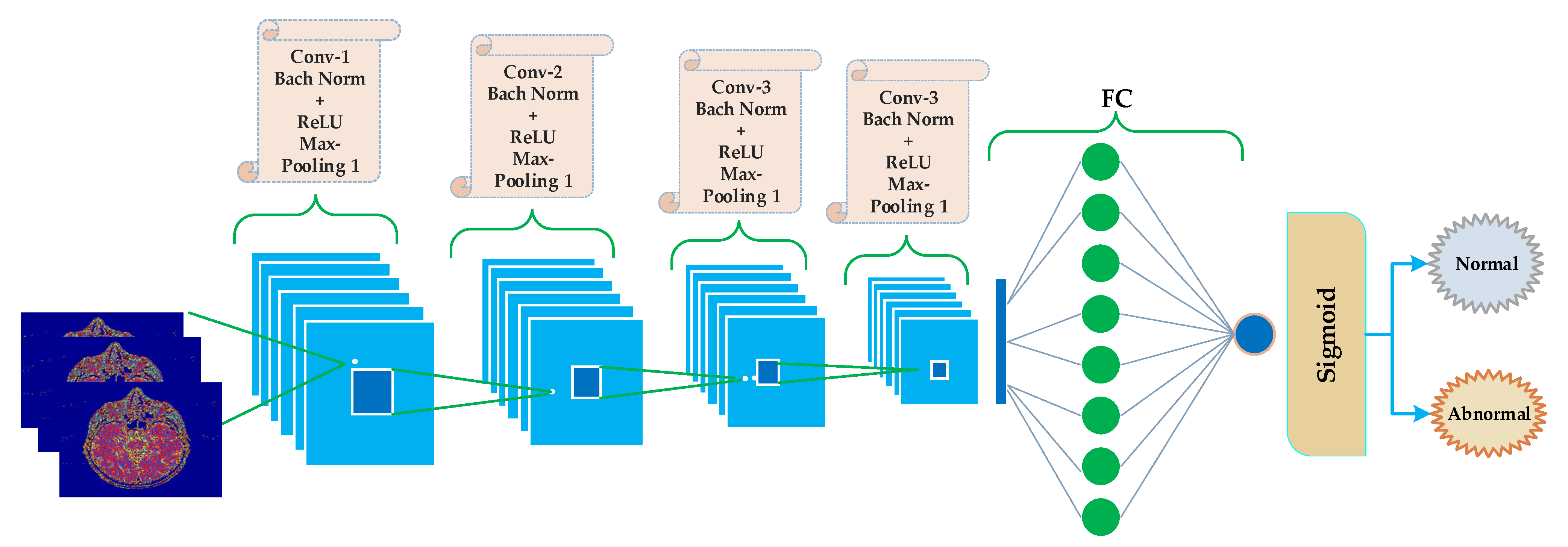
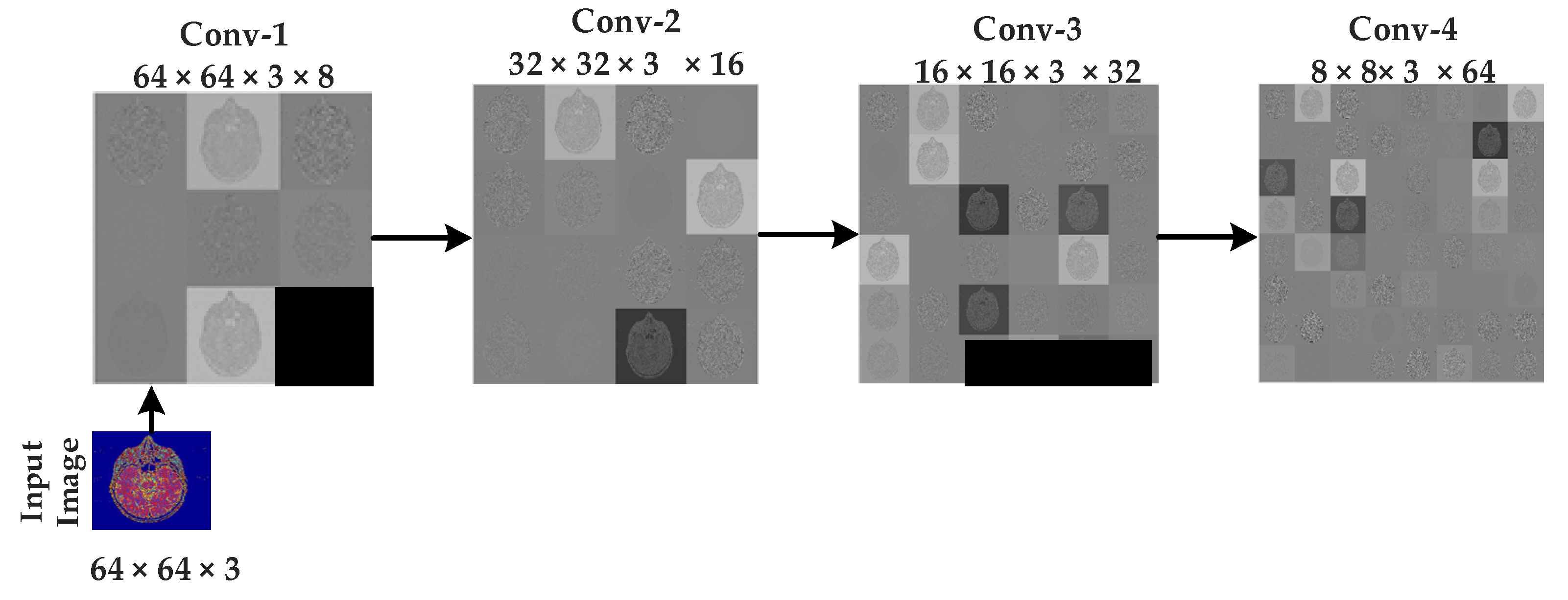
3.3. Convolutional Neural Networks (CNNs)
4. Implementation, Results, and Explanations
4.1. Implementation Setup
4.2. Results and Discussion
5. Conclusions and Future Work
Author Contributions
Funding
Institutional Review Board Statement
Informed Consent Statement
Data Availability Statement
Conflicts of Interest
References
- Strogatz, S.H. Exploring complex networks. Nature 2001, 40, 268–276. [Google Scholar] [CrossRef] [Green Version]
- Newman, M.E.J. Assortative Mixing in Networks. Phys. Rev. Lett. 2002, 89, 208701. [Google Scholar] [CrossRef] [PubMed] [Green Version]
- Boccaletti, S.; Latora, V.; Moreno, Y.; Chavez, M.; Hwang, D.-U. Complex networks: Structure and dynamics. Phys. Rep. 2006, 424, 175–308. [Google Scholar] [CrossRef]
- Rubinov, M.; Sporns, O. Complex network measures of brain connectivity: Uses and interpretations. NeuroImage 2010, 52, 1059–1069. [Google Scholar] [CrossRef] [PubMed]
- Pessoa, L. Understanding brain networks and brain organization. Phys. Life Rev. 2014, 11, 400–435. [Google Scholar] [CrossRef] [PubMed] [Green Version]
- Hagmann, P.; Kurant, M.; Gigandet, X.; Thiran, P.; Wedeen, V.J.; Meuli, R.; Thiran, J.-P. Mapping Human Whole-Brain Structural Networks with Diffusion MRI. PLoS ONE 2007, 2, e597. [Google Scholar] [CrossRef] [Green Version]
- He, Y.; Chen, Z.J.; Evans, A.C. Small-World Anatomical Networks in the Human Brain Revealed by Cortical Thickness from MRI. Cereb. Cortex 2007, 17, 2407–2419. [Google Scholar] [CrossRef] [Green Version]
- Tohka, J.; Zijdenbos, A.; Evans, A. Fast and robust parameter estimation for statistical partial volume models in brain MRI. NeuroImage 2004, 23, 84–97. [Google Scholar] [CrossRef] [PubMed] [Green Version]
- Ahmad, M.; Shafi, I.; Osman, A. Classification of Tumors in Human Brain MRI using Wavelet and Support Vector Machine. IOSR J. Comput. Eng. 2012, 8, 25–31. [Google Scholar] [CrossRef]
- El-Dahshan, E.-S.A.; Mohsen, H.M.; Revett, K.; Salem, A.-B.M. Computer-aided diagnosis of human brain tumor through MRI: A survey and a new algorithm. Expert Syst. Appl. 2014, 41, 5526–5545. [Google Scholar] [CrossRef]
- Gillies, R.J.; Kinahan, P.E.; Hricak, H. Radiomics: Images Are More than Pictures, They Are Data. Radiology 2016, 278, 563–577. [Google Scholar] [CrossRef] [Green Version]
- Lehmann, T.M.; Bredno, J. Strategies to Configure Image Analysis Algorithms for Clinical Usage. J. Am. Med. Inform. Assoc. 2005, 12, 497–504. [Google Scholar] [CrossRef] [Green Version]
- Shen, S.; Sandham, W.; Granat, M.; Sterr, A. MRI Fuzzy Segmentation of Brain Tissue Using Neighborhood Attraction with Neural-Network Optimization. IEEE Trans. Inf. Technol. Biomed. 2005, 9, 459–467. [Google Scholar] [CrossRef] [PubMed] [Green Version]
- Remedios, S.; Roy, S.; Pham, D.L.; Butman, J.A. Classifying magnetic resonance image modalities with convolutional neural networks. In Medical Imaging 2018: Computer-Aided Diagnosis; SPIE: Bellingham, WA, USA, 2018; Volume 10575, p. 105752I. [Google Scholar]
- Akkus, Z.; Galimzianova, A.; Hoogi, A.; Rubin, D.L.; Erickson, B.J. Deep Learning for Brain MRI Segmentation: State of the Art and Future Directions. J. Digit. Imaging 2017, 30, 449–459. [Google Scholar] [CrossRef] [Green Version]
- Yuan, L.; Wei, X.; Shen, H.; Zeng, L.-L.; Hu, D. Multi-Center Brain Imaging Classification Using a Novel 3D CNN Approach. IEEE Access 2018, 6, 49925–49934. [Google Scholar] [CrossRef]
- Yasaka, K.; Akai, H.; Kunimatsu, A.; Kiryu, S.; Abe, O. Deep learning with convolutional neural network in radiology. Jpn. J. Radiol. 2018, 36, 257–272. [Google Scholar] [CrossRef] [PubMed]
- Bernal, J.; Kushibar, K.; Asfaw, D.S.; Valverde, S.; Oliver, A.; Martí, R.; Lladó, X. Deep convolutional neural networks for brain image analysis on magnetic resonance imaging: A review. Artif. Intell. Med. 2019, 95, 64–81. [Google Scholar] [CrossRef] [PubMed] [Green Version]
- Othman, M.F.; Abdullah, N.B.; Kamal, N.F. MRI brain classification using support vector machine. In Proceedings of the 2011 Fourth International Conference on Modeling, Simulation and Applied Optimization, Kuala Lumpur, Malaysia, 19–21 April 2011. [Google Scholar]
- Fletcher-Heath, L.M.; Hall, L.O.; Goldgof, D.B.; Murtagh, F. Automatic segmentation of non-enhancing brain tumors in magnetic resonance images. Artif. Intell. Med. 2001, 21, 43–63. [Google Scholar] [CrossRef] [Green Version]
- Gilanie, G.; Bajwa, U.I.; Waraich, M.M.; Habib, Z.; Ullah, H.; Nasir, M.; Bajwa, U.I. Classification of normal and abnormal brain MRI slices using Gabor texture and support vector machines. Signal Image Video Process. 2017, 12, 479–487. [Google Scholar] [CrossRef]
- Ezhang, Y.; Edong, Z.; Ephillips, P.; Wang, S.; Eji, G.; Eyang, J.; Yuan, T.-F. Detection of subjects and brain regions related to Alzheimer’s disease using 3D MRI scans based on eigenbrain and machine learning. Front. Comput. Neurosci. 2015, 9, 66. [Google Scholar] [CrossRef] [Green Version]
- Shen, D.; Wu, G.; Suk, H.-I. Deep Learning in Medical Image Analysis. Annu. Rev. Biomed. Eng. 2017, 19, 221–248. [Google Scholar] [CrossRef] [Green Version]
- Fayaz, M.; Shah, A.S.; Wahid, F.; Shah, A. A Robust Technique of Brain MRI Classification using Color Features and K-Nearest Neighbors Algorithm. Int. J. Signal Process. Image Process. Pattern Recognit. 2016, 9, 11–20. [Google Scholar] [CrossRef]
- Chaplot, S.; Patnaik, L.; Jagannathan, N.R. Classification of magnetic resonance brain images using wavelets as input to support vector machine and neural network. Biomed. Signal Process. Control. 2006, 1, 86–92. [Google Scholar] [CrossRef]
- Zhang, Y.-D.; Wang, S.; Huo, Y.; Wu, L.; Liu, A. Feature extraction of brain mri by stationary wavelet transform and its applications. J. Biol. Syst. 2010, 18, 115–132. [Google Scholar] [CrossRef]
- Shah, A.S.; Khan, M.; Subhan, F.; Fayaz, M.; Shah, A. An Offline Signature Verification Technique Using Pixels Intensity Levels. Int. J. Signal Process. Image Process. Pattern Recognit. 2016, 9, 205–222. [Google Scholar] [CrossRef]
- Ortiz, A.; Górriz, J.; Ramírez, J.; Salas-González, D.; Llamas-Elvira, J. Two fully-unsupervised methods for MR brain image segmentation using SOM-based strategies. Appl. Soft Comput. 2013, 13, 2668–2682. [Google Scholar] [CrossRef]
- Nath, M.K.; Sahambi, J. Independent component analysis of functional MRI data. In Proceedings of the TENCON 2008—2008 IEEE Region 10 Conference, Hyderabad, India, 19–21 November 2008; pp. 1–6. [Google Scholar]
- Saritha, M.; Joseph, K.P.; Mathew, A.T. Classification of MRI brain images using combined wavelet entropy based spider web plots and probabilistic neural network. Pattern Recognit. Lett. 2013, 34, 2151–2156. [Google Scholar] [CrossRef]
- Maitra, M.; Chatterjee, A. A Slantlet transform based intelligent system for magnetic resonance brain image classification. Biomed. Signal Process. Control. 2006, 1, 299–306. [Google Scholar] [CrossRef]
- Peper, J.S.; Brouwer, R.M.; Boomsma, D.I.; Kahn, R.S.; Pol, H.E.H. Genetic influences on human brain structure: A review of brain imaging studies in twins. Hum. Brain Mapp. 2007, 28, 464–473. [Google Scholar] [CrossRef] [PubMed]
- Kharrat, A.; Benamrane, N. A Hybrid Approach for Automatic Classification of Brain MRI Using Genetic Algorithm and Support Vector Machine Mesh Region Classification View project Imagerie et vision artificielle View project. Leonardo J. Sci. 2010, 17, 71–82. [Google Scholar]
- Zhang, Y.; Dong, Z.; Wu, L.; Wang, S. A hybrid method for MRI brain image classification. Expert Syst. Appl. 2011, 38, 10049–10053. [Google Scholar] [CrossRef]
- Chen, R.-M.; Yang, S.-C.; Wang, C.-M. MRI brain tissue classification using unsupervised optimized extenics-based methods. Comput. Electr. Eng. 2017, 58, 489–501. [Google Scholar] [CrossRef]
- Mallick, P.K.; Ryu, S.H.; Satapathy, S.K.; Mishra, S.; Nguyen, G.N.; Tiwari, P. Brain MRI Image Classification for Cancer Detection Using Deep Wavelet Autoencoder-Based Deep Neural Network. IEEE Access 2019, 7, 46278–46287. [Google Scholar] [CrossRef]
- Ismael, S.A.A.; Mohammed, A.; Hefny, H. An enhanced deep learning approach for brain cancer MRI images classification using residual networks. Artif. Intell. Med. 2020, 102, 101779. [Google Scholar] [CrossRef]
- Maitra, M.; Chatterjee, A.; Matsuno, F. A novel scheme for feature extraction and classification of magnetic resonance brain images based on Slantlet Transform and Support Vector Machine. In Proceedings of the 2008 IEEE SICE Annual Conference, Yokyo, Japan, 20–22 August 2008; pp. 1130–1134. [Google Scholar]
- Kumar, S.; Dabas, C.; Godara, S. Classification of Brain MRI Tumor Images: A Hybrid Approach. Procedia Comput. Sci. 2017, 122, 510–517. [Google Scholar] [CrossRef]
- El-Dahshan, E.-S.A.; Hosny, T.; Salem, A.-B.M. Hybrid intelligent techniques for MRI brain images classification. Digit. Signal Process. 2010, 20, 433–441. [Google Scholar] [CrossRef]
- Mohsen, H.; El-Dahshan, E.-S.A.; El-Horbaty, E.-S.M.; Salem, A.-B.M. Classification using deep learning neural networks for brain tumors. Futur. Comput. Inform. J. 2018, 3, 68–71. [Google Scholar] [CrossRef]
- Wahid, F.; Ghazali, R.; Fayaz, M.; Shah, A.S. Using Probabilistic Classification Technique and Statistical Features for Brain Magnetic Resonance Imaging (MRI) Classification: An Application of AI Technique in Bio-Science. Int. J. Bio-Sci. Bio-Technol. 2017, 8, 93–106. [Google Scholar] [CrossRef]
- Ullah, Z.; Lee, S.-H.; Fayaz, M. Enhanced feature extraction technique for brain MRI classification based on Haar wavelet and statistical moments. Int. J. Adv. Appl. Sci. 2019, 6, 89–98. [Google Scholar] [CrossRef]
- Amin, J.; Sharif, M.; Gul, N.; Yasmin, M.; Shad, S.A. Brain tumor classification based on DWT fusion of MRI sequences using convolutional neural network. Pattern Recognit. Lett. 2020, 129, 115–122. [Google Scholar] [CrossRef]
- Maqsood, S.; Damasevicius, R.; Shah, F.M. An Efficient Approach for the Detection of Brain Tumor Using Fuzzy Logic and U-NET CNN Classification. In Proceedings of the International Conference on Computational Science and Its Applications; Springer: Cham, Switzerland, 2021; pp. 105–118. [Google Scholar]
- Muzammil, S.; Maqsood, S.; Haider, S.; Damaševičius, R. CSID: A Novel Multimodal Image Fusion Algorithm for Enhanced Clinical Diagnosis. Diagnostics 2020, 10, 904. [Google Scholar] [CrossRef] [PubMed]
- Odusami, M.; Maskeliūnas, R.; Damaševičius, R.; Krilavičius, T. Analysis of Features of Alzheimer’s Disease: Detection of Early Stage from Functional Brain Changes in Magnetic Resonance Images Using a Finetuned ResNet18 Network. Diagnostics 2021, 11, 1071. [Google Scholar] [CrossRef] [PubMed]
- Zhang, Y.-D.; Zhao, G.; Sun, J.; Wu, X.; Wang, Z.-H.; Liu, H.-M.; Govindaraj, V.V.; Zhan, T.; Li, J. Smart pathological brain detection by synthetic minority oversampling technique, extreme learning machine, and Jaya algorithm. Multimed. Tools Appl. 2018, 77, 22629–22648. [Google Scholar] [CrossRef]
- Hemanth, D.J.; Anitha, J.; Naaji, A.; Geman, O.; Popescu, D.E.; Son, L.H. A Modified Deep Convolutional Neural Network for Abnormal Brain Image Classification. IEEE Access 2019, 7, 4275–4283. [Google Scholar] [CrossRef]
- Simonyan, K.; Zisserman, A. Very deep convolutional networks for large-scale image recognition. arXiv 2014, arXiv:1409.1556. [Google Scholar]
- Kamnitsas, K.; Ledig, C.; Newcombe, V.; Simpson, J.P.; Kane, A.D.; Menon, D.K.; Rueckert, D.; Glocker, B. Efficient multi-scale 3D CNN with fully connected CRF for accurate brain lesion segmentation. Med. Image Anal. 2017, 36, 61–78. [Google Scholar] [CrossRef]
- Pereira, S.; Pinto, A.; Alves, V.; Silva, C. Brain Tumor Segmentation Using Convolutional Neural Networks in MRI Images. IEEE Trans. Med. Imaging 2016, 35, 1240–1251. [Google Scholar] [CrossRef]
- Liu, Y.; Stojadinovic, S.; Hrycushko, B.; Wardak, Z.; Lau, S.; Lu, W.; Yan, Y.; Jiang, S.B.; Zhen, X.; Timmerman, R.; et al. A deep convolutional neural network-based automatic delineation strategy for multiple brain metastases stereotactic radiosurgery. PLoS ONE 2017, 12, e0185844. [Google Scholar] [CrossRef] [Green Version]
- Toğaçar, M.; Cömert, Z.; Ergen, B. Classification of brain MRI using hyper column technique with convolutional neural network and feature selection method. Expert Syst. Appl. 2020, 149, 113274. [Google Scholar] [CrossRef]
- Çinar, A.; Yildirim, M. Detection of tumors on brain MRI images using the hybrid convolutional neural network architecture. Med. Hypotheses 2020, 139, 109684. [Google Scholar] [CrossRef] [PubMed]
- Saxena, P.; Maheshwari, A.; Maheshwari, S. Predictive Modeling of Brain Tumor: A Deep Learning Approach. In Innovations in Computational Intelligence and Computer Vision; Springer: Singapore, 2021; pp. 275–285. [Google Scholar]
- Khan, H.; Shah, P.M.; Shah, M.A.; Islam, S.U.; Rodrigues, J. Cascading handcrafted features and Convolutional Neural Network for IoT-enabled brain tumor segmentation. Comput. Commun. 2020, 153, 196–207. [Google Scholar] [CrossRef]
- Kruthika, K.R.; Maheshappa, H. CBIR system using Capsule Networks and 3D CNN for Alzheimer’s disease diagnosis. Inform. Med. Unlocked 2019, 14, 59–68. [Google Scholar] [CrossRef]
- Chang, J.; Zhang, L.; Gu, N.; Zhang, X.; Ye, M.; Yin, R.; Meng, Q. A mix-pooling CNN architecture with FCRF for brain tumor segmentation. J. Vis. Commun. Image Represent. 2019, 58, 316–322. [Google Scholar] [CrossRef]
- Talo, M.; Yildirim, O.; Baloglu, U.B.; Aydin, G.; Acharya, U.R. Convolutional neural networks for multi-class brain disease detection using MRI images. Comput. Med Imaging Graph. 2019, 78, 101673. [Google Scholar] [CrossRef] [PubMed]
- Nazir, M.; Wahid, F.; Khan, S.A. A simple and intelligent approach for brain MRI classification. J. Intell. Fuzzy Syst. 2015, 28, 1127–1135. [Google Scholar] [CrossRef]
- Nanni, L.; Lumini, A. Wavelet decomposition tree selection for palm and face authentication. Pattern Recognit. Lett. 2008, 29, 343–353. [Google Scholar] [CrossRef]
- Schmeelk, J. Wavelet transforms on two-dimensional images. Math. Comput. Model. 2002, 36, 939–948. [Google Scholar] [CrossRef]
- Available online: http://www.med.harvard.edu/AANLIB/home.html (accessed on 15 February 2021).
- Das, S.; Aranya, O.R.; Labiba, N.N. Brain tumor classification using convolutional neural network. In Proceedings of the 2019 1st International Conference on Advances in Science, Engineering and Robotics Technology (ICASERT), Dhaka, Bangladesh, 3 May 2019; pp. 1–5. [Google Scholar]
- Zweig, M.H.; Campbell, G. Receiver-operating characteristic (ROC) plots: A fundamental evaluation tool in clinical medicine. Clin. Chem. 1993, 39, 561–577. [Google Scholar] [CrossRef]
- Cheng, J.; Yang, W.; Huang, M.; Huang, W.; Jiang, J.; Zhou, Y.; Yang, R.; Zhao, J.; Feng, Y.; Feng, Q.; et al. Retrieval of Brain Tumors by Adaptive Spatial Pooling and Fisher Vector Representation. PLoS ONE 2016, 11, e0157112. [Google Scholar] [CrossRef] [PubMed]
- Rajini, N.H.; Bhavani, R. Classification of MRI brain images using k-nearest neighbor and artificial neural network. In Proceedings of the IEEE 2011 International Conference on Recent Trends in Information Technology (ICRTIT), Chennai, India, 3–5 June 2011; pp. 563–568. [Google Scholar]
- Kabir-Anaraki, A.; Ayati, M.; Kazemi, F. Magnetic resonance imaging-based brain tumor grades classification and grading via convolutional neural networks and genetic algorithms. Biocybern. Biomed. Eng. 2019, 39, 63–74. [Google Scholar] [CrossRef]
- Liu, D.; Liu, Y.; Dong, L. G-ResNet: Improved ResNet for brain tumor classification. In Proceedings of the International Conference on Neural Information Processing (ICONIP), Sydney, NSW, Australia, 12 December 2019; pp. 535–545. [Google Scholar]
- Ghosal, P.; Nandanwar, L.; Kanchan, S.; Bhadra, A.; Chakraborty, J.; Nandi, D. Brain tumor classi_cation using ResNet-101 based squeeze and excitation deep neural network. In Proceedings of the 2019 Second International Conference on Advanced Computational and Communication Paradigms (ICACCP), Gangtok, India, 25–28 February 2019; pp. 1–6. [Google Scholar]
- Shi, J.; Li, Z.; Ying, S.; Wang, C.; Liu, Q.; Zhang, Q.; Yan, P. MR image super-resolution via wide residual networks with fixed skip connection. IEEE J. Biomed. Health Informat. 2019, 23, 1129–1140. [Google Scholar] [CrossRef]
- Wang, Y.; Yan, J.; Sun, Q.; Li, J.; Yang, Z. A MobileNets Convolutional Neural Network for GIS Partial Discharge Pattern Recognition in the Ubiquitous Power Internet of Things Context: Optimization, Comparison, and Application. IEEE Access 2019, 7, 150226–150236. [Google Scholar] [CrossRef]


| Notation | Description |
|---|---|
| CNN | Convolutional Neural Network |
| DWT | Discrete Wavelet Transform |
| CT | Computed tomography |
| MRI | Magnetic Resonance Imaging |
| ReLU | Rectified linear unit |
| Cov | Convolution |
| LL | Low-Low Level Detail |
| HL | High-Low Level Detail |
| LH | Low-High Detail |
| HH | High-High Level Detail |
| FC | Fully Connected |
| TP | True Positive |
| TN | True Negative |
| PF | False Positive |
| ROC | Receiver Operating Characteristic |
| VEs | Validation Errors |
| Reference | Model | Contribution | Limitation |
|---|---|---|---|
| [14] | Integrated model of CNN and Transfer Learning | Good classification accuracy on test data. | Very large and complex CNN model |
| [16] | Novel 3D CNN Method | Robust when training on one dataset and testing on another dataset. | Only designed for 3D images, and low classification accuracy |
| [36] | Autoencoder Deep Neural Network (ADNN) | Accuracy was improved | High Computation Complexity |
| [37] | Enhanced Approach using Residual Networks | High accuracy was achieved by considering small dataset. | Poor results on large dataset |
| [49] | Modified Deep Convolutional Neural Network | Computation complexity was reduced | Low classification accuracy |
| [60] | AlexNet, Vgg-16, ResNet18, ResNet34, and ResNet50 | Used to classify five classes (normal, cerebrovascular, neoplastic, degenerative, and inflammatory) | Low classification accuracy |
| [61] | Color Moments and artificial neural network | Simple and very fast | Low classification accuracy |
| [43] | DWT, color moments, and artificial neural network | High accuracy | Good only on small dataset |
| Number | Layer Name | Layer Properties |
|---|---|---|
| 1 | Images (Input) | Size = 64 × 64 × 3 |
| 2 | Conv-1 | Convolutional (64 × 64 × 3 × 8) with stride 2 |
| 3 | Bach Norm | Bach Normalization Operation |
| 4 | ReLU | Rectified Linear Unit |
| 5 | Max Pooling | Max-Pooling Operation (2 × 2, stride [2,2], padding = [same]) |
| 6 | Dropout | 50% dropout |
| 7 | Conv-2 | Convolutional (32 × 32 × 3 × 16) with stride 2 |
| 8 | Bach Norm | Bach Normalization Operation |
| 9 | ReLU | Rectified Linear Unit |
| 10 | Max Pooling | Max-Pooling Operation (2 × 2, stride [2,2]) |
| 11 | Dropout | 50% dropout |
| 12 | Conv-3 | Convolutional (16 × 16 × 3 × 32, stride 2, padding = [0,0,0,0]) |
| 13 | Bach Norm | Bach Normalization Operation |
| 14 | ReLU | Rectified Linear Unit |
| 15 | Max Pooling | Max-Pooling Operation (2 × 2, stride [2,2], padding = [same]) |
| 16 | Dropout | 50% |
| 17 | Conv-4 | Convolutional (8 × 8 × 3 × 64) with stride 2 |
| 18 | Bach Norm | Bach Normalization Operation |
| 19 | ReLU | Rectified Linear Unit |
| 20 | Max Pooling | Max-Pooling Operation (2 × 2, stride [2,2], padding = [same]) |
| 21 | Dropout | 50% |
| 22 | Fully Connected | 512 hidden neurons in first hidden layer and 1024 in second hidden layer |
| 23 | Functions | tanh on first and second hidden layers neurons, and sigmoid on the output layer neuron. |
| 24 | Classification | Output (Normal or abnormal) |
| 25 | Loss | Binary Cross-entropy |
| Max Epochs | Validity Frequency | Learning Rate |
|---|---|---|
| 35 | 31 | 0.001 |
| Total Number of CNN Layers | Validation Error |
|---|---|
| 6 | 0.12125 |
| 10 | 0.11358 |
| 20 | 0.10889 |
| 25 | 0.08000 |
| 30 | 0.09835 |
| 35 | 0.10486 |
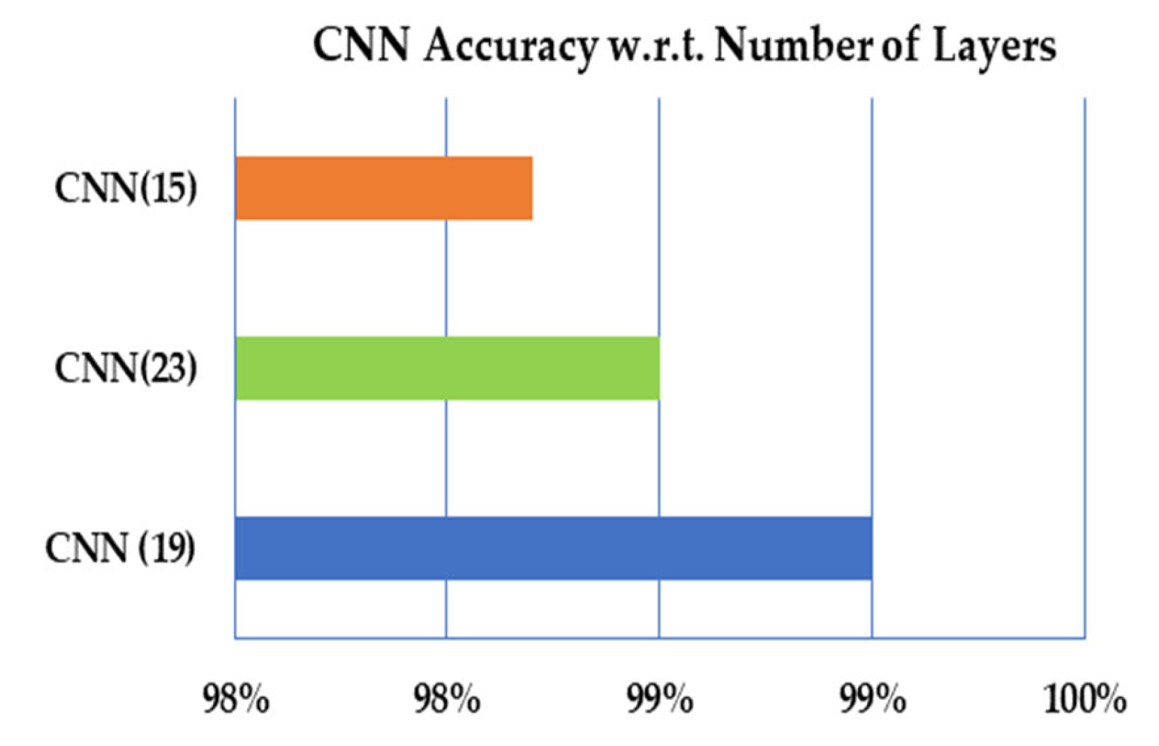
| CNN (No. Layers) | Kappa Statistics | TP Rate | FP Rate | AUC | Recall | Precision |
|---|---|---|---|---|---|---|
| CNN (19) | 0.9880 | 0.990 | 0.0013 | 0.9970 | 0.9970 | 0.9980 |
| CNN (23) | 0.9820 | 0.9850 | 0.0030 | 0.9990 | 0.9860 | 0.9880 |
| SVM (15) | 0.9780 | 0.9820 | 0.0040 | 0.9990 | 0.9804 | 0.9881 |
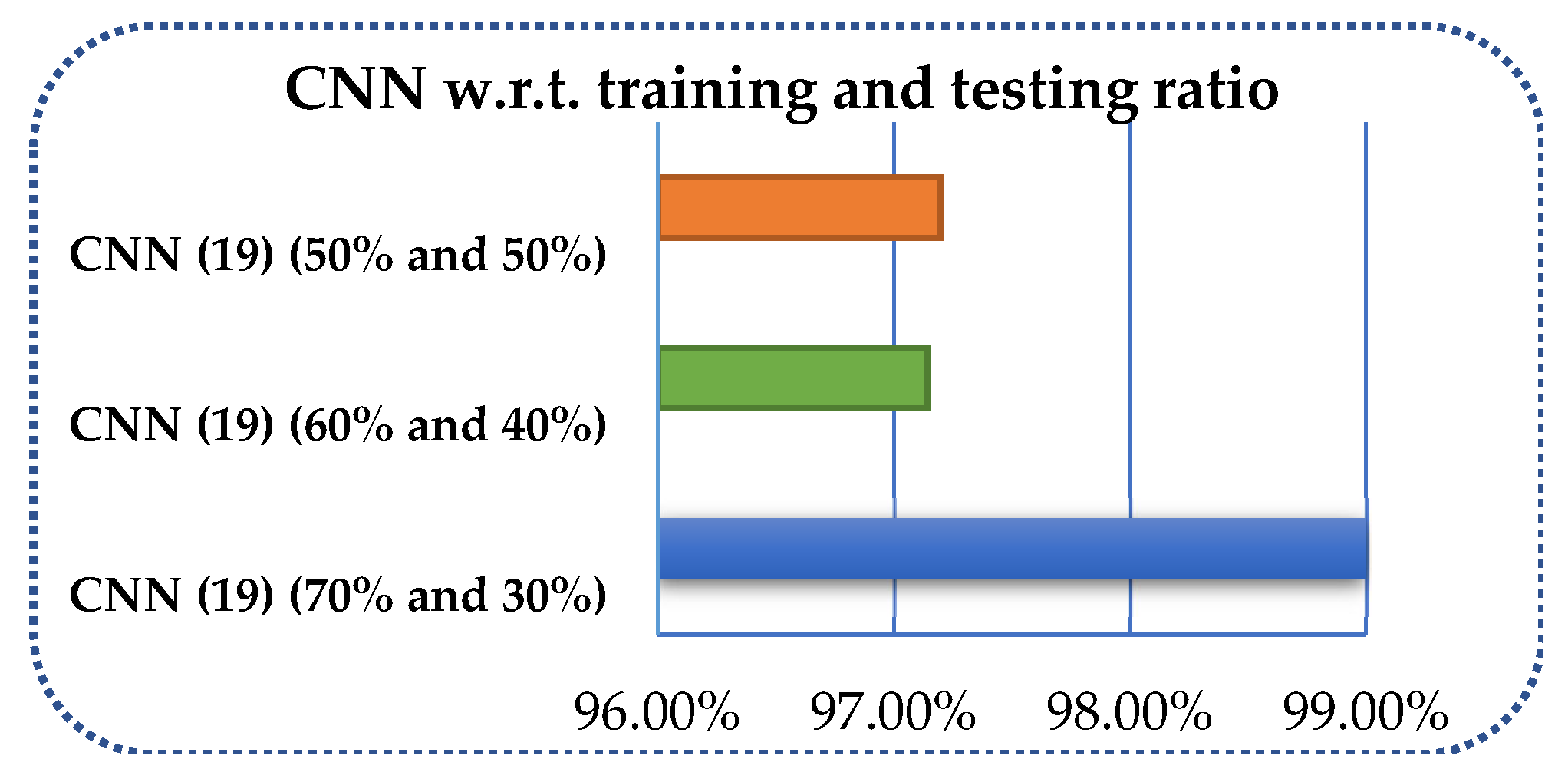
| Method (Ratio) | Kappa Statistics | TP Rate | FP Rate | ROC | Recall | Precision |
|---|---|---|---|---|---|---|
| CNN (19) (70 and 30%) | 0.9880 | 0.990 | 0.0020 | 0.997 | 0.990 | 0.990 |
| CNN (19) (60 and 40%) | 0.93780 | 0.96150 | 0.03850 | 1 | 0.96150 | 97.14209 |
| CNN (19) (50 and 50%) | 0.96530 | 0.971 | 0.0060 | 0.9970 | 0.9710 | 0.9720 |
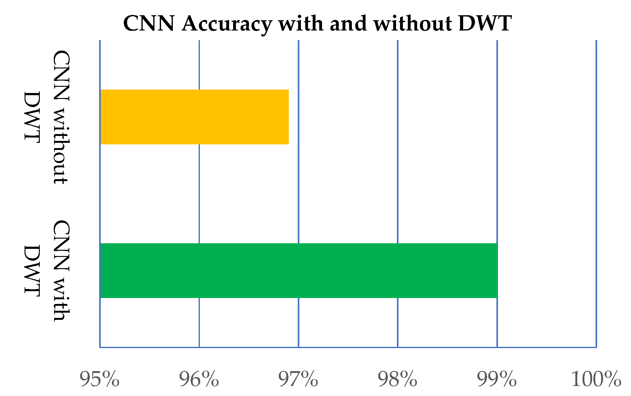
| CNN (No. Layers) | Kappa Statistics | TP Rate | FP Rate | ROC | Recall | Precision |
|---|---|---|---|---|---|---|
| CNN (19) with DWT | 0.9880 | 0.99 | 0.0020 | 0.9970 | 0.99 | 0.99 |
| CNN (19) without DWT | 0.9627 | 0.969 | 0.0060 | 0.998 | 0.9690 | 0.9690 |
| Model | Training Accuracy | Testing Accuracy | Training Minimum Loss | Testing Minimum Loss |
|---|---|---|---|---|
| CNNBCN-ER [61] | 100.00% | 94.85% | 1.43 × 10⁻³ | 1.86 × 10⁻¹ |
| CNNBCN-WS [61] | 100.00% | 94.53% | 6.61 × 10⁻⁴ | 2.20 × 10⁻¹ |
| CNNBCN-BA [61] | 100.00% | 94.53% | 1.43 × 10⁻³ | 1.72 × 10⁻¹ |
| CNNBCN-ER1 [61] | 100.00% | 95.49% | 1.07 × 10⁻³ | 1.69 × 10⁻¹ |
| CNNBCN-WS1 [61] | 100.00% | 95.17% | 1.46 × 10⁻³ | 2.13 × 10⁻¹ |
| CNNBCN-BA1 [61] | 100.00% | 95.01% | 1.13 × 10⁻³ | 1.71 × 10⁻¹ |
| Model 1 [68] | − | 91.28% | − | − |
| Model 2 [67] | − | 94.68% | − | − |
| Model 3 [69] | 99.54% | 94.20% | 2.53 × 10⁻² | 1.82 × 10⁻¹ |
| Model 4 [65] | − | 94.39% | − | |
| Model 5 [70] | − | 95.00% | − | − |
| Model 6 [71] | − | 93.83% | − | − |
| Wide-Resnet-101 [72] | 99.51% | 91.14% | 1.72 × 10⁻² | 2.90 × 10⁻¹ |
| Mobilenet-v1 [73] | 100.00% | 93.88% | 2.96 × 10⁻³ | 2.23 × 10⁻¹ |
| Proposed Method | 100.00% | 97.32% | 3.42 × 10⁻⁴ | 1.53 × 10⁻¹ |
Publisher’s Note: MDPI stays neutral with regard to jurisdictional claims in published maps and institutional affiliations. |
© 2021 by the authors. Licensee MDPI, Basel, Switzerland. This article is an open access article distributed under the terms and conditions of the Creative Commons Attribution (CC BY) license (https://creativecommons.org/licenses/by/4.0/).
Share and Cite
Fayaz, M.; Torokeldiev, N.; Turdumamatov, S.; Qureshi, M.S.; Qureshi, M.B.; Gwak, J. An Efficient Methodology for Brain MRI Classification Based on DWT and Convolutional Neural Network. Sensors 2021, 21, 7480. https://doi.org/10.3390/s21227480
Fayaz M, Torokeldiev N, Turdumamatov S, Qureshi MS, Qureshi MB, Gwak J. An Efficient Methodology for Brain MRI Classification Based on DWT and Convolutional Neural Network. Sensors. 2021; 21(22):7480. https://doi.org/10.3390/s21227480
Chicago/Turabian StyleFayaz, Muhammad, Nurlan Torokeldiev, Samat Turdumamatov, Muhammad Shuaib Qureshi, Muhammad Bilal Qureshi, and Jeonghwan Gwak. 2021. "An Efficient Methodology for Brain MRI Classification Based on DWT and Convolutional Neural Network" Sensors 21, no. 22: 7480. https://doi.org/10.3390/s21227480
APA StyleFayaz, M., Torokeldiev, N., Turdumamatov, S., Qureshi, M. S., Qureshi, M. B., & Gwak, J. (2021). An Efficient Methodology for Brain MRI Classification Based on DWT and Convolutional Neural Network. Sensors, 21(22), 7480. https://doi.org/10.3390/s21227480