
A Spectrum Correction Algorithm Based on Beat Signal of FMCW Laser Ranging System


Abstract
:1. Introduction
- (1)
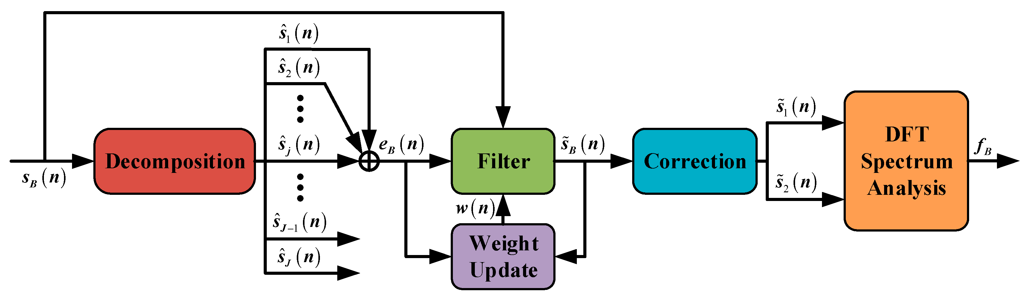
- This algorithm reduces the influence of WGN, affecting the correction accuracy. In the decomposition and filter part, the beat signal is divided into several components, and each component has its characteristics in the frequency domain. Among them, the first few components possess the widest frequency coverage, and there are no obvious peaks in their power spectrum. The sum can be used as the input of the filter, and the WGN in the beat signal will be mostly removed with the weight parameter.
- (2)
- This algorithm minimizes the impact of spectrum leakage effectively. The Hann window has a narrow main lobe, low side lobe, and fast attenuation speed from the main lobe to the first side lobe. Using two Hann windows in the correction part can concentrate more energy of the signal, thereby making the spectral peak of the desired frequency more obvious.
- (3)
- This algorithm diminishes the picket fence effect that may decrease the frequency resolution of the beat signal. We utilize phase values and the delay value of two signals in the frequency domain after DFT processing. The phase values correspond to the spectral peaks that are at the same position in these signals. Therefore, the calculation error caused by broad adjacent spectral lines near the peak in only one used signal is avoided, and an accurate frequency value of the beat signal is obtained.
- (4)
- This algorithm is different from the traditional spectrum correction algorithm, which can reduce the influence caused by WGN, spectrum leakage, and the picket fence effect at the same time, so that the frequency value obtained by this algorithm is more accurate and the distance ranged by this system is more precise.
2. Methods
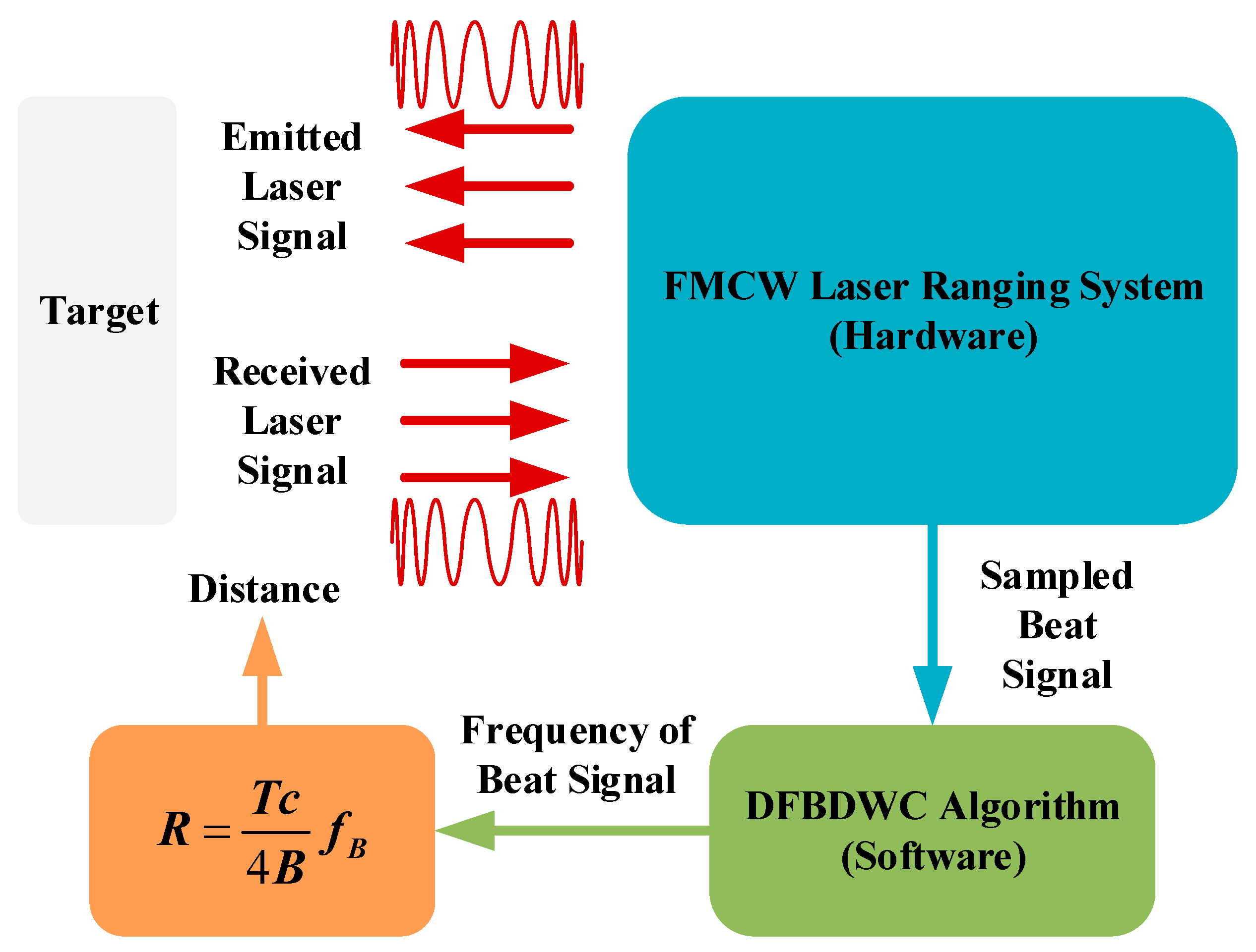
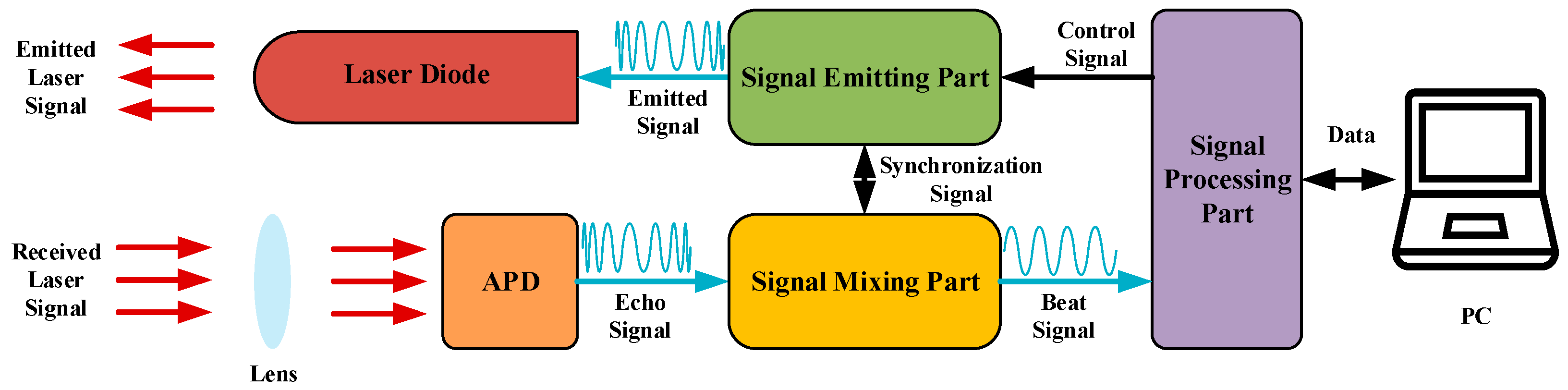
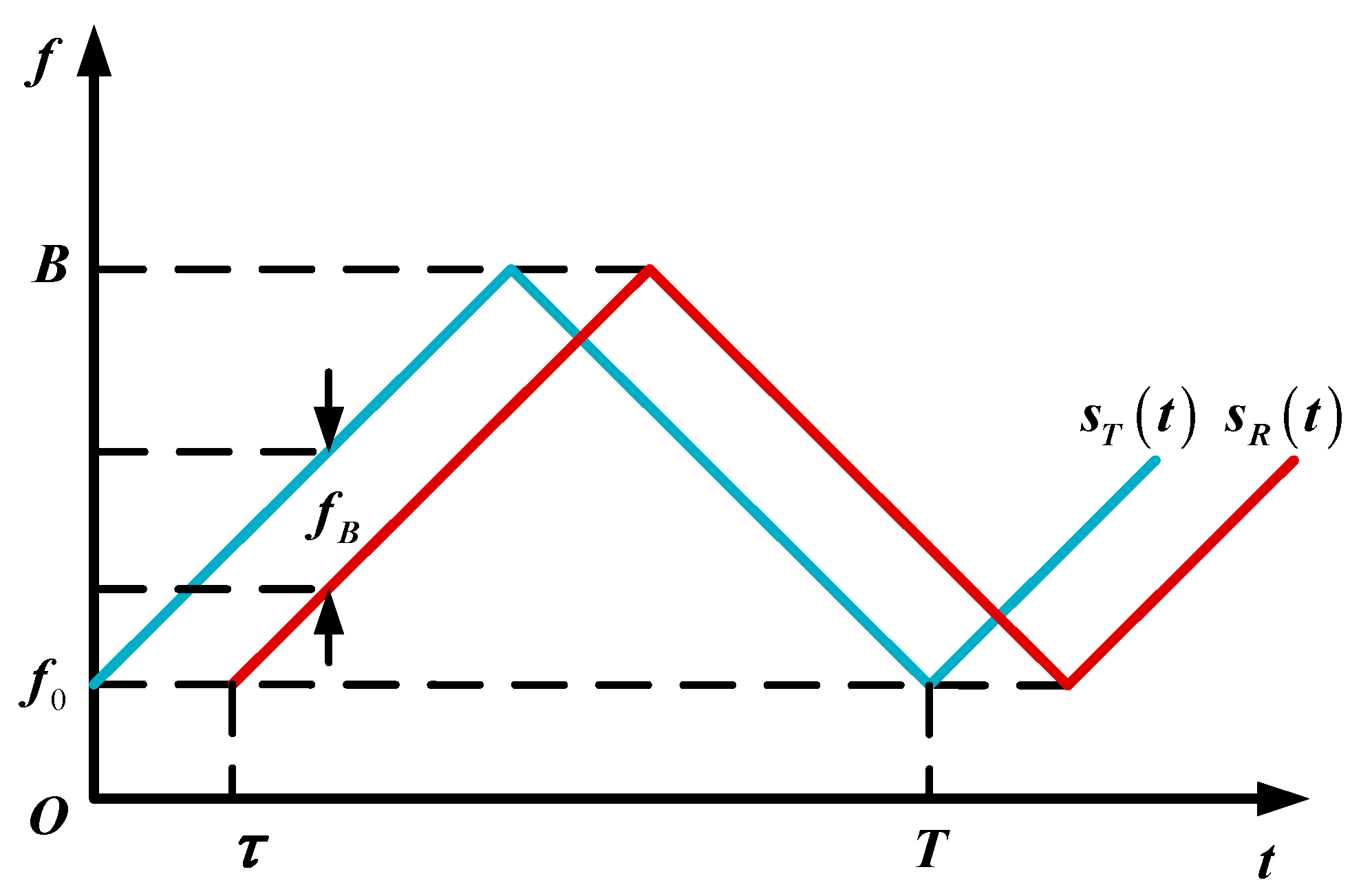
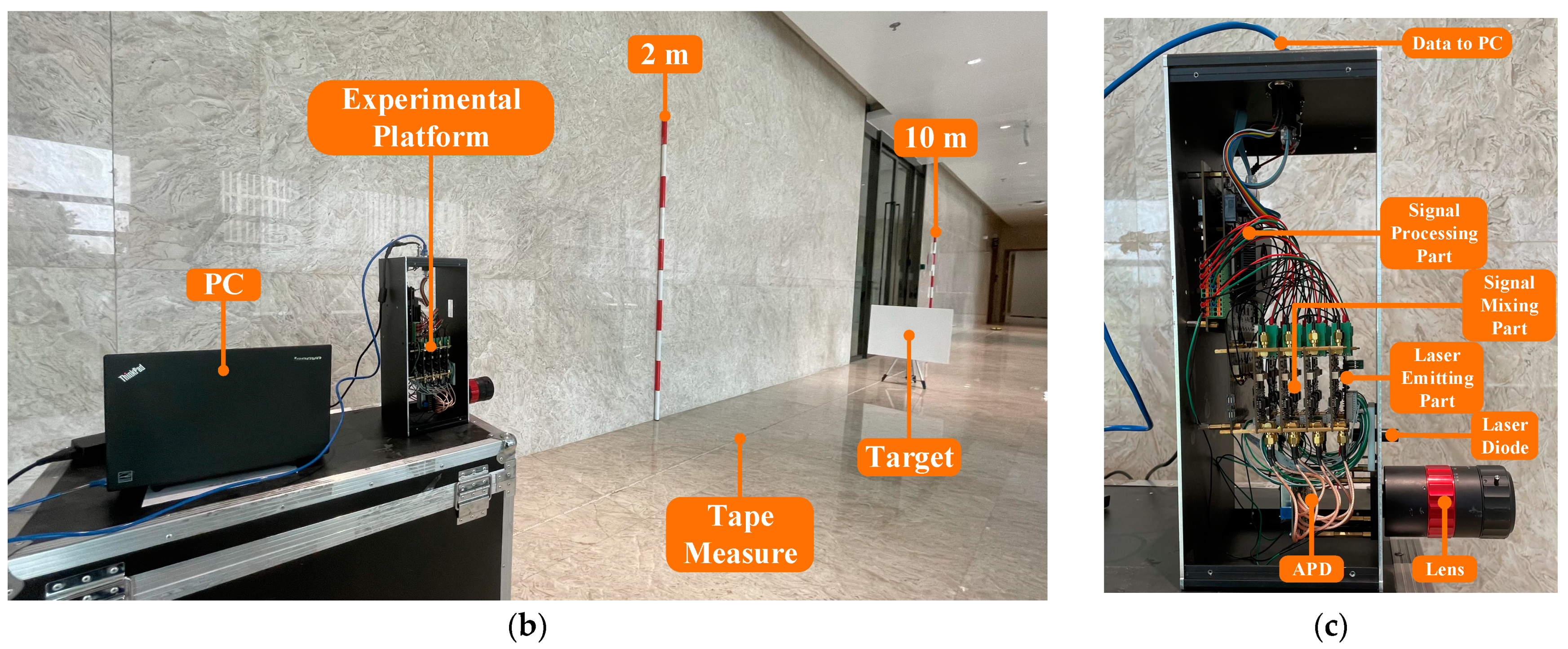
2.1. FMCW Laser Ranging System
2.2. DFBDWC Algorithm
3. Results and Discussion
3.1. Simulation
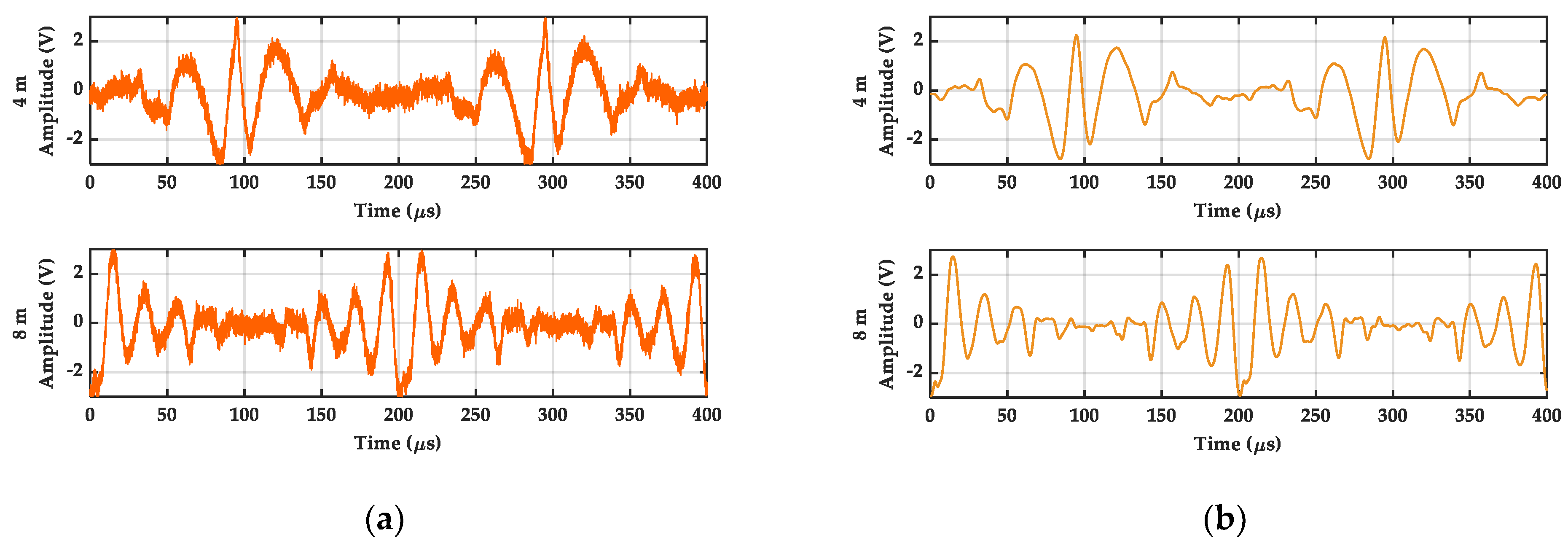
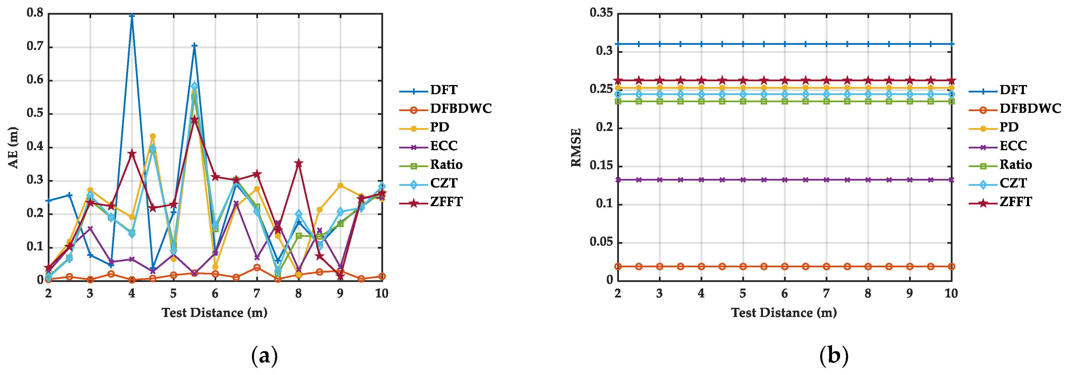
3.2. Experiment
4. Conclusions
Author Contributions
Funding
Institutional Review Board Statement
Informed Consent Statement
Data Availability Statement
Conflicts of Interest
References
- Amann, M.C.; Bosch, T.; Lescure, M.; Myllyla, R.; Rioux, M. Laser ranging: A critical review of usual techniques for distance measurement. Opt. Eng. 2001, 40, 10–19. [Google Scholar]
- Borkowski, J.; Mroczka, J. LIDFT method with classic data windows and zero padding in multifrequency signal analysis. Measurement 2010, 43, 1595–1602. [Google Scholar] [CrossRef]
- Rife, D.C.; Vincent, G.A. Use of the discrete Fourier transform in the measurement of frequencies and levels of tones. Bell Syst. Tech. J. 1970, 49, 197–228. [Google Scholar] [CrossRef]
- Grandke, T. Interpolation algorithms for discrete Fourier transforms of weighted signals. IEEE Trans. Instrum. Meas. 1983, 32, 350–355. [Google Scholar] [CrossRef]
- Ming, X.; Kang, D. Corrections for frequency, amplitude and phase in a fast Fourier transform of a harmonic signal. Mech. Syst. Signal Proc. 1996, 10, 211–221. [Google Scholar] [CrossRef]
- Agrez, D. Weighted multipoint interpolated DFT to improve amplitude estimation of multifrequency signal. IEEE Trans. Instrum. Meas. 2002, 51, 287–292. [Google Scholar] [CrossRef]
- Belega, D.; Dallet, D. Frequency estimation via weighted multipoint interpolated DFT. IET Sci. Meas. Technol. 2008, 2, 1–8. [Google Scholar] [CrossRef]
- Belega, D.; Dallet, D. Multifrequency signal analysis by interpolated DFT method with maximum sidelobe decay windows. Measurement 2009, 42, 420–426. [Google Scholar] [CrossRef]
- Belega, D.; Dallet, D.; Petri, D. Accuracy of sine wave frequency estimation by multipoint interpolated DFT approach. IEEE Trans. Instrum. Meas. 2010, 59, 2808–2815. [Google Scholar] [CrossRef]
- Mcmahon, D.R.A.; Barrett, R.F. An efficient method for the estimation of the frequency of a single tone in noise from the phases of discrete Fourier transforms. Signal Process. 1986, 11, 169–177. [Google Scholar] [CrossRef]
- Zhu, L.; Li, H.; Ding, H.; Xiong, Y. Noise influence on estimation of signal parameter from the phase difference of discrete Fourier transforms. Mech. Syst. Signal Proc. 2002, 16, 991–1004. [Google Scholar] [CrossRef]
- Kang, D.; Ming, X.; Xiaofei, Z. Phase difference correction method for phase and frequency in spectral analysis. Mech. Syst. Signal Proc. 2000, 14, 835–843. [Google Scholar] [CrossRef]
- Luo, J.; Xie, M. Phase difference methods based on asymmetric windows. Mech. Syst. Signal Proc. 2015, 54/55, 52–67. [Google Scholar] [CrossRef]
- Ding, K.; Cao, D.; Li, W. An approach to discrete spectrum correction based on energy centroid. Key Eng. Mater. 2006, 321-323, 1270–1273. [Google Scholar]
- Offelli, C.; Petri, D. A frequency-domain procedure for accurate real-time signal parameter measurement. IEEE Trans. Instrum. Meas. 1990, 39, 363–368. [Google Scholar] [CrossRef]
- Belega, D.; Dallet, D.; Petri, D. Accuracy of the normalized frequency estimation of a discrete-time sine-wave by the energy-based method. IEEE Trans. Instrum. Meas. 2012, 61, 111–121. [Google Scholar] [CrossRef]
- Lin, H.; Ding, K. Energy based signal parameter estimation method and a comparative study of different frequency estimators. Mech. Syst. Signal Proc. 2011, 25, 452–464. [Google Scholar]
- Zhang, Q.; Zhong, S.; Lin, J.; Huang, Y.; Nsengiyumva, W.; Chen, W.; Luo, M.; Zhong, J.; Yu, Y.; Peng, Z.; et al. Anti-noise frequency estimation performance of Hanning-windowed energy centrobaric method for optical coherence velocimeter. Opt. Lasers Eng. 2020, 134. [Google Scholar] [CrossRef]
- Rabiner, L.; Schafer, R.; Rader, C. The chirp z-transform algorithm. IEEE Trans. Audio Electroacoust. 1969, 17, 86–92. [Google Scholar] [CrossRef]
- Leng, J.; Shan, C. Application of chirp-z transformation in high accuracy measurement of radar. Appl. Mech. Mater. 2013, 392, 730–733. [Google Scholar] [CrossRef]
- Li, D.; Liu, H.; Liao, Y.; Gui, X. A novel helicopter-borne rotating SAR imaging model and algorithm based on inverse chirp-z transform using frequency-modulated continuous wave. IEEE Geosci. Remote Sens. Lett. 2015, 12, 1625–1629. [Google Scholar]
- Masso, E.; Bolognini, N. Dynamic multiple-image encryption based on chirp z-transform. J. Opt. 2019, 21, 035704. [Google Scholar] [CrossRef]
- Qin, M.; Li, D.; Tang, X.; Zeng, C.; Li, W.; Xu, L. A fast high-resolution imaging algorithm for helicopter-borne rotating array SAR based on 2-D chirp-z transform. Remote Sens. 2019, 11, 1669. [Google Scholar] [CrossRef] [Green Version]
- Shen, S.; Nie, X.; Tang, L.; Bai, Y.; Zhang, X.; Li, L.; Ben, D. An improved coherent integration method for wideband radar based on two-dimensional frequency correction. Electronics 2020, 9, 840. [Google Scholar] [CrossRef]
- Wei, D.; Nagata, Y.; Aketagawa, M. Partial phase reconstruction for zero optical path difference determination using a chirp z-transform-based algorithm. Opt. Commun. 2020, 463, 125456. [Google Scholar] [CrossRef]
- Lyons, R.G. The Zoom FFT. In Understanding Digital Signal Processing, 3rd ed.; Bernard, G., Ed.; Pearson Education: Boston, MA, USA, 2011; pp. 548–550. [Google Scholar]
- Al-Qudsi, B.; Joram, N.; Strobel, A.; Ellinger, F. Zoom FFT for precise spectrum calculation in FMCW radar using FPGA. In Proceedings of the 2013 9th Conference on Ph.D. Research in Microelectronics and Electronics, Villach, Austria, 24–27 June 2013. [Google Scholar]
- Huang, N.E.; Shen, Z.; Long, S.R.; Wu, M.C.; Shih, H.H.; Zheng, Q.; Yen, N.C.; Tung, C.C.; Liu, H.H. The empirical mode decomposition and the Hilbert spectrum for nonlinear and non-stationary time series analysis. Proc. R. Soc. A Math. Phys. Eng. Sci. 1998, 454, 903–995. [Google Scholar] [CrossRef]
- Torres, M.E.; Colominas, M.A.; Schlotthauer, G.; Flandrin, P. A complete ensemble empirical mode decomposition with adaptive noise. In Proceedings of the IEEE International Conference on Acoustics, Speech, and Signal Processing (ICASSP), Prague Congress Center, Prague, Czech Republic, 22–27 May 2011. [Google Scholar]
- Colominas, M.A.; Schlotthauer, G.; Torres, M.E. Improved complete ensemble EMD: A suitable tool for biomedical signal processing. Biomed. Signal Process. Control. 2014, 14, 19–29. [Google Scholar] [CrossRef]
- Diniz, P.S.R. Adaptive Filtering: Algorithms and Practical Implementation, 5th ed.; Springer Nature: Cham, Switzerland, 2020; pp. 157–160. [Google Scholar]
- Huang, X.; Wang, Z.; Hou, G. New method of estimation of phase, amplitude, and frequency based on all phase FFT spectrum analysis. In Proceedings of the IEEE 2007 International Symposium on Intelligent Signal Processing and Communication Systems, Xiamen, China, 28 November–1 December 2007. [Google Scholar]
- Su, T.; Yang, M.; Jin, T.; Flesch, R.C.C. Power harmonic and interharmonic detection method in renewable power based on Nuttall double-window all-phase FFT algorithm. IET Renew. Power Gener. 2018, 12, 953–961. [Google Scholar] [CrossRef]
- Zhang, D.; Sun, S.; Zhao, H.; Yang, J. Laser Doppler dignal processing based on trispectral interpolation of Nuttall window. Optik 2019, 205, 163364. [Google Scholar] [CrossRef]
- Lin, H.C. Power harmonics and interharmonics measurement using recursive group-harmonic power minimizing algorithm. IEEE Trans. Ind. Electron. 2012, 59, 1184–1193. [Google Scholar] [CrossRef]


| Parameter | Interpretation | Value |
|---|---|---|
| The amplitude decay rate of echo signal | 0.8 | |
| The amplitude of emitted signal | 1 | |
| The initial frequency | 1 MHz | |
| The speed of light | 299,792,458 m/s | |
| The modulation bandwidth | 99 MHz | |
| The modulation period | 200 μs | |
| The sample rate | 20 MHz | |
| The upper limit frequency | 0.8 | |
| The lower limit frequency | 1 |
| Lower Limit (m) | Test Distance (m) | Upper Limit (m) | ||||||||
|---|---|---|---|---|---|---|---|---|---|---|
| 1.5141 | 2 | 3 | 4 | 5 | 6 | 7 | 8 | 9 | 10 | 22.7115 |
| 2.5 | 3.5 | 4.5 | 5.5 | 6.5 | 7.5 | 8.5 | 9.5 | |||
| Test Distance (Real Distance) (m) | Computed Distance (m) | ||||||
|---|---|---|---|---|---|---|---|
| DFT | PD | ECC | Ratio | CZT | ZFFT | DFBDWC | |
| 2 | 1.8483 | 2.2712 | 2.0092 | 2.0162 | 2.0109 | 2.1230 | 2.0021 |
| 2.5 | 2.3103 | 2.5013 | 2.4898 | 2.5102 | 2.5136 | 2.5121 | 2.5011 |
| 3 | 3.2345 | 2.9997 | 3.0018 | 2.9977 | 3.0164 | 2.9354 | 3.0004 |
| 3.5 | 3.6965 | 3.5102 | 3.5163 | 3.5118 | 3.5191 | 3.6794 | 3.5038 |
| 4 | 4.1586 | 3.9989 | 3.9992 | 4.0074 | 3.9923 | 4.0685 | 4.0003 |
| 4.5 | 4.6207 | 4.4945 | 4.4967 | 4.4939 | 4.5246 | 4.4919 | 4.4981 |
| 5 | 5.0827 | 4.9836 | 5.0128 | 5.0064 | 4.9977 | 4.8810 | 4.9988 |
| 5.5 | 5.5448 | 5.4979 | 5.4977 | 5.5069 | 5.5005 | 5.6250 | 5.5021 |
| 6 | 6.0069 | 5.9938 | 5.9968 | 5.9938 | 6.0032 | 6.0141 | 6.0028 |
| 6.5 | 6.4689 | 6.5056 | 6.5119 | 6.5053 | 6.5059 | 6.4374 | 6.4969 |
| 7 | 6.9310 | 6.9930 | 6.9942 | 7.0027 | 7.0086 | 6.8265 | 7.0017 |
| 7.5 | 7.3931 | 7.4954 | 7.4987 | 7.4968 | 7.5114 | 7.5705 | 7.5032 |
| 8 | 7.8552 | 7.9956 | 8.0202 | 8.0079 | 8.0141 | 7.9939 | 8.0022 |
| 8.5 | 8.3172 | 8.5020 | 8.5015 | 8.5079 | 8.5168 | 8.3830 | 8.4985 |
| 9 | 8.7793 | 8.9948 | 9.0008 | 8.9943 | 9.0196 | 9.1270 | 9.0030 |
| 9.5 | 9.7034 | 9.5065 | 9.5206 | 9.5043 | 9.4927 | 9.5161 | 9.4996 |
| 10 | 10.1655 | 9.9997 | 10.0038 | 10.0056 | 9.9954 | 9.9394 | 10.0027 |
| Test Distance (Real Distance) (m) | AE (cm) | ||||||
|---|---|---|---|---|---|---|---|
| DFT | PD | ECC | Ratio | CZT | ZFFT | DFBDWC | |
| 2 | 15.1729 | 27.1155 | 0.7593 | 1.6049 | 1.0918 | 12.2982 | 0.0064 |
| 2.5 | 18.9662 | 0.3612 | 0.5100 | 1.2172 | 1.3648 | 1.2092 | 0.0066 |
| 3 | 23.4474 | 0.1285 | 0.0044 | 0.3879 | 1.6378 | 6.4557 | 0.0118 |
| 3.5 | 19.6541 | 0.4905 | 0.9653 | 0.9247 | 1.9107 | 17.9420 | 0.0069 |
| 4 | 15.8609 | 0.0843 | 0.4251 | 0.7488 | 0.7735 | 6.8530 | 0.0112 |
| 4.5 | 12.0677 | 0.1837 | 0.0044 | 0.3630 | 2.4567 | 0.8119 | 0.0022 |
| 5 | 8.2744 | 0.0604 | 1.1222 | 0.6495 | 0.2276 | 11.9009 | 0.0109 |
| 5.5 | 4.4812 | 0.1957 | 0.3470 | 0.5298 | 0.0453 | 12.4969 | 0.0273 |
| 6 | 0.6880 | 0.2423 | 0.0084 | 0.3479 | 0.3183 | 1.4078 | 0.0087 |
| 6.5 | 3.1053 | 0.2089 | 1.2866 | 0.5007 | 0.5913 | 6.2571 | 0.0013 |
| 7 | 6.8985 | 0.2696 | 0.2793 | 0.4013 | 0.8642 | 17.3461 | 0.0036 |
| 7.5 | 10.6917 | 0.3016 | 0.0156 | 0.3363 | 1.1372 | 7.0517 | 0.0027 |
| 8 | 14.4850 | 0.2962 | 1.4637 | 0.4075 | 1.4102 | 0.6132 | 0.0093 |
| 8.5 | 18.2782 | 0.3348 | 0.2210 | 0.3157 | 1.2741 | 11.7023 | 0.0044 |
| 9 | 22.0714 | 0.3613 | 0.0266 | 0.3265 | 1.9561 | 12.6955 | 0.0084 |
| 9.5 | 20.3421 | 0.3672 | 1.6550 | 0.3435 | 0.7282 | 1.6065 | 0.0054 |
| 10 | 16.5489 | 0.3971 | 0.1714 | 0.2539 | 0.4552 | 6.0584 | 0.0024 |
| Test Distance (Real Distance) (m) | Computed Distance (m) | ||||||
|---|---|---|---|---|---|---|---|
| DFT | PD | ECC | Ratio | CZT | ZFFT | DFBDWC | |
| 2 | 2.2406 | 2.0378 | 2.0288 | 2.0142 | 2.0112 | 2.0405 | 1.9947 |
| 2.5 | 2.2428 | 2.3821 | 2.3995 | 2.4305 | 2.4324 | 2.3972 | 2.5130 |
| 3 | 3.0778 | 3.2725 | 3.1569 | 3.2413 | 3.2570 | 3.2344 | 3.0044 |
| 3.5 | 3.4525 | 3.2725 | 3.4428 | 3.3091 | 3.3091 | 3.2757 | 3.4788 |
| 4 | 4.7937 | 4.1913 | 3.9345 | 4.1448 | 4.1420 | 4.3819 | 4.0037 |
| 4.5 | 4.5397 | 4.9340 | 4.5286 | 4.8935 | 4.8972 | 4.7189 | 4.4921 |
| 5 | 4.7935 | 4.9340 | 5.0797 | 4.8935 | 4.9086 | 4.7702 | 5.0177 |
| 5.5 | 4.7951 | 4.9340 | 5.4775 | 4.9486 | 4.9170 | 5.0159 | 5.5240 |
| 6 | 6.0848 | 6.0423 | 6.0834 | 6.1554 | 6.1661 | 6.3121 | 5.9786 |
| 6.5 | 6.7901 | 6.7241 | 6.2667 | 6.8037 | 6.7990 | 6.8023 | 6.5111 |
| 7 | 6.7856 | 6.7241 | 7.0700 | 6.7772 | 6.7912 | 6.6798 | 6.9593 |
| 7.5 | 7.5608 | 7.6350 | 7.6754 | 7.5213 | 7.5307 | 7.6526 | 7.5062 |
| 8 | 7.8234 | 7.9807 | 7.9655 | 7.8641 | 7.7992 | 7.6465 | 8.0192 |
| 8.5 | 8.3899 | 8.7136 | 8.3474 | 8.3670 | 8.3959 | 8.5749 | 8.5271 |
| 9 | 9.1752 | 8.7136 | 9.0420 | 9.1708 | 9.2079 | 9.0146 | 8.9694 |
| 9.5 | 9.7220 | 9.7542 | 9.7507 | 9.7275 | 9.7192 | 9.7459 | 9.4933 |
| 10 | 9.7324 | 9.7542 | 9.7507 | 9.7374 | 9.7163 | 9.7367 | 10.0143 |
| DFT | PD | ECC | Ratio | CZT | ZFFT | DFBDWC | |
|---|---|---|---|---|---|---|---|
| Maximum (m) | 0.7937 | 0.5660 | 0.2507 | 0.5514 | 0.5830 | 0.4841 | 0.0407 |
| Minimum (m) | 0.0397 | 0.0193 | 0.0225 | 0.0142 | 0.0112 | 0.0146 | 0.0037 |
| Sample Time (μs) | Computation Time Consuming (s) | ||||||
|---|---|---|---|---|---|---|---|
| DFT | PD | ECC | Ratio | CZT | ZFFT | DFBDWC | |
| 100 | 0.0423 | 0.0449 | 0.0458 | 0.0452 | 0.0441 | 0.0243 | 2.3891 |
| 200 | 0.0444 | 0.0501 | 0.0468 | 0.0464 | 0.0460 | 0.0259 | 5.6616 |
Publisher’s Note: MDPI stays neutral with regard to jurisdictional claims in published maps and institutional affiliations. |
© 2021 by the authors. Licensee MDPI, Basel, Switzerland. This article is an open access article distributed under the terms and conditions of the Creative Commons Attribution (CC BY) license (https://creativecommons.org/licenses/by/4.0/).
Share and Cite
Hao, Y.; Song, P.; Wang, X.; Pan, Z. A Spectrum Correction Algorithm Based on Beat Signal of FMCW Laser Ranging System. Sensors 2021, 21, 5057. https://doi.org/10.3390/s21155057
Hao Y, Song P, Wang X, Pan Z. A Spectrum Correction Algorithm Based on Beat Signal of FMCW Laser Ranging System. Sensors. 2021; 21(15):5057. https://doi.org/10.3390/s21155057
Chicago/Turabian StyleHao, Yi, Ping Song, Xuanquan Wang, and Zhikang Pan. 2021. "A Spectrum Correction Algorithm Based on Beat Signal of FMCW Laser Ranging System" Sensors 21, no. 15: 5057. https://doi.org/10.3390/s21155057
APA StyleHao, Y., Song, P., Wang, X., & Pan, Z. (2021). A Spectrum Correction Algorithm Based on Beat Signal of FMCW Laser Ranging System. Sensors, 21(15), 5057. https://doi.org/10.3390/s21155057