
Anomaly Detection and Automatic Labeling for Solar Cell Quality Inspection Based on Generative Adversarial Network


Abstract
:1. Introduction
2. Related Works
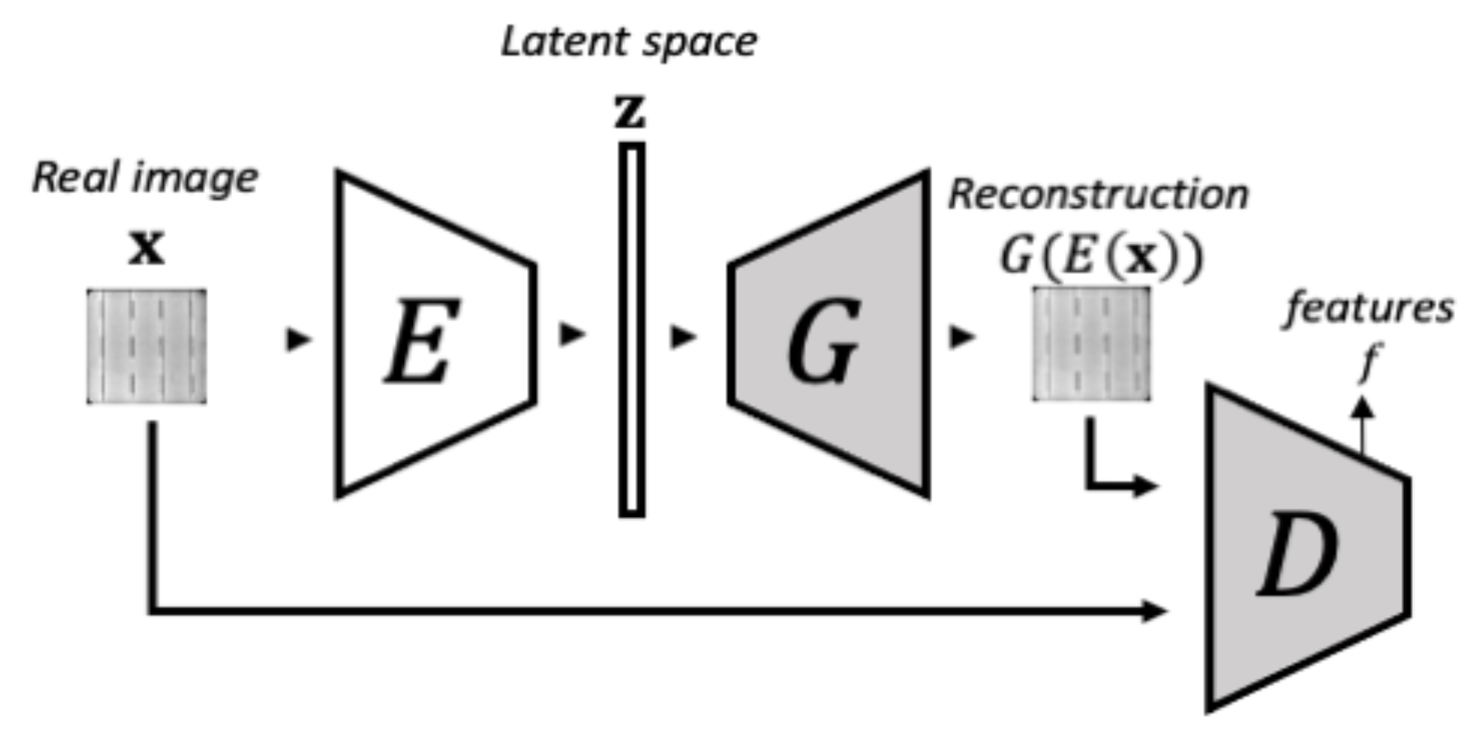
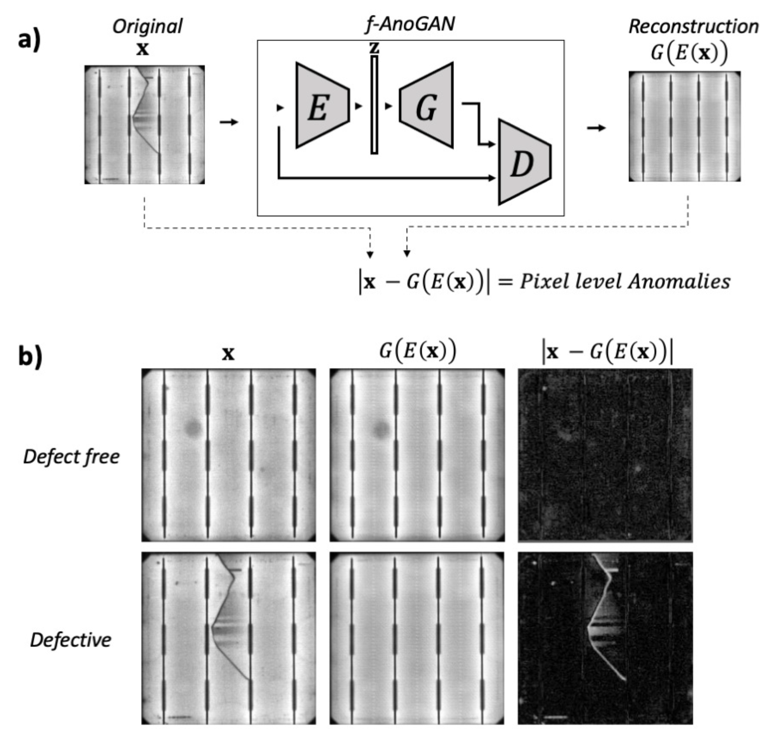
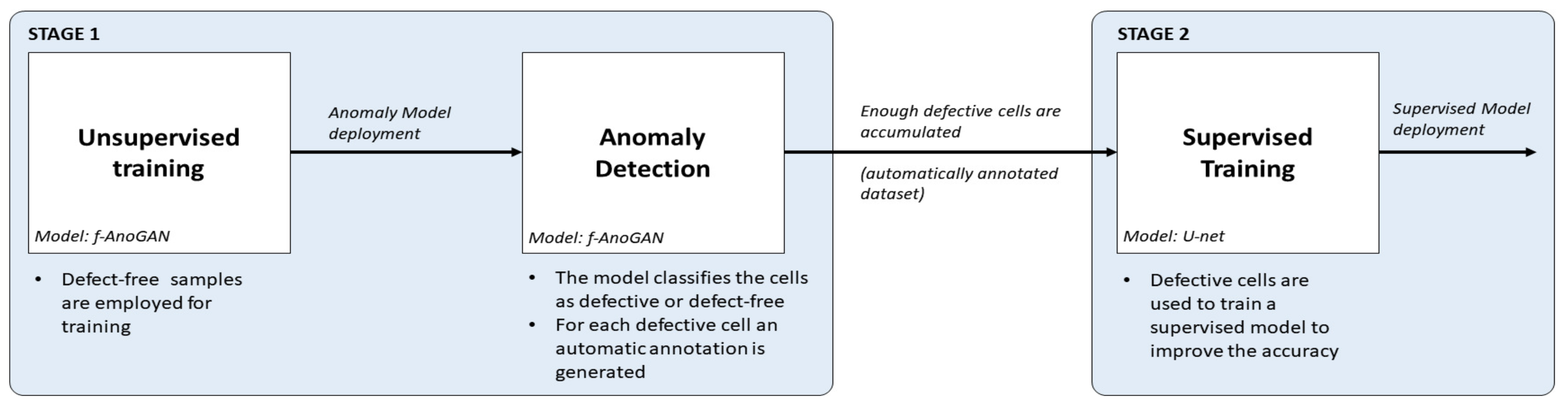
- First, using an anomaly detection approach, defect-free samples can be employed to obtain an initial inspection model that from the very beginning of a new production line can detect and segment anomalies in EL images of cells. For this purpose, f-AnoGAN [41], a GAN-based anomaly detection network that has been shown to work well with medical images, is adapted for inspection. The original architecture has been modified such that instead of using a sliding window method, the images can be processed as a whole, reducing the processing time drastically. In addition, a modified training scheme is proposed which improves the defect detection rates with respect to the results with the original training scheme.
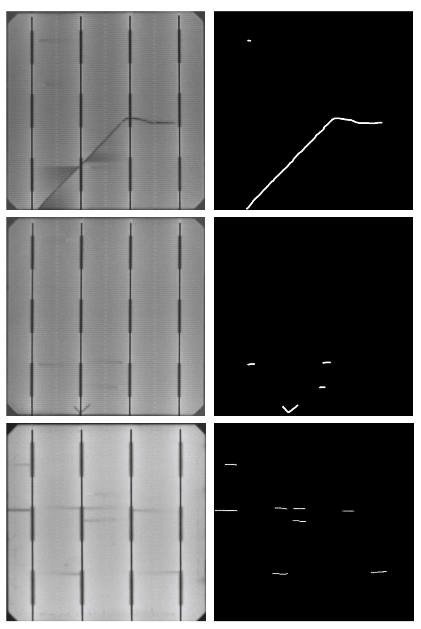
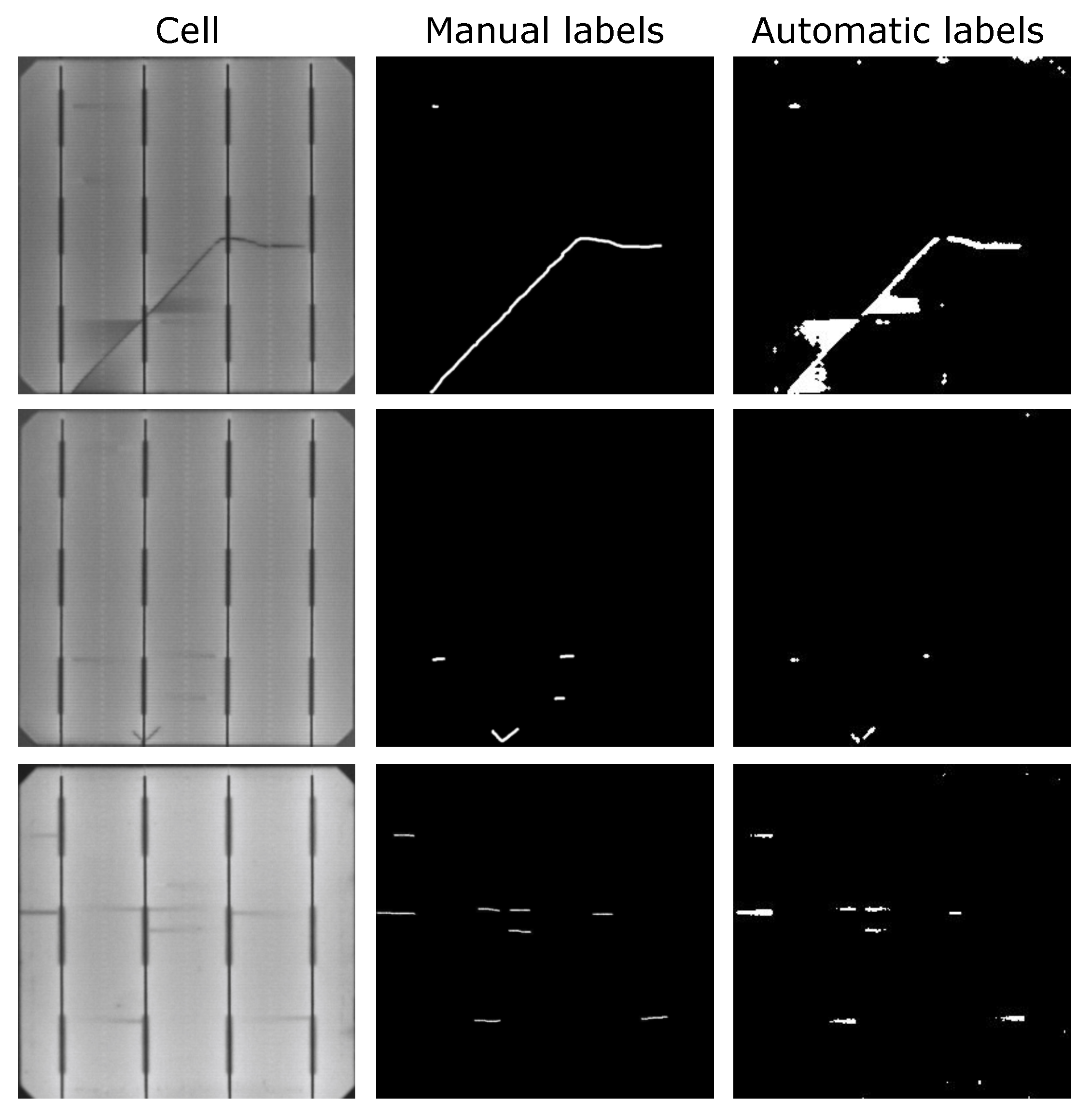
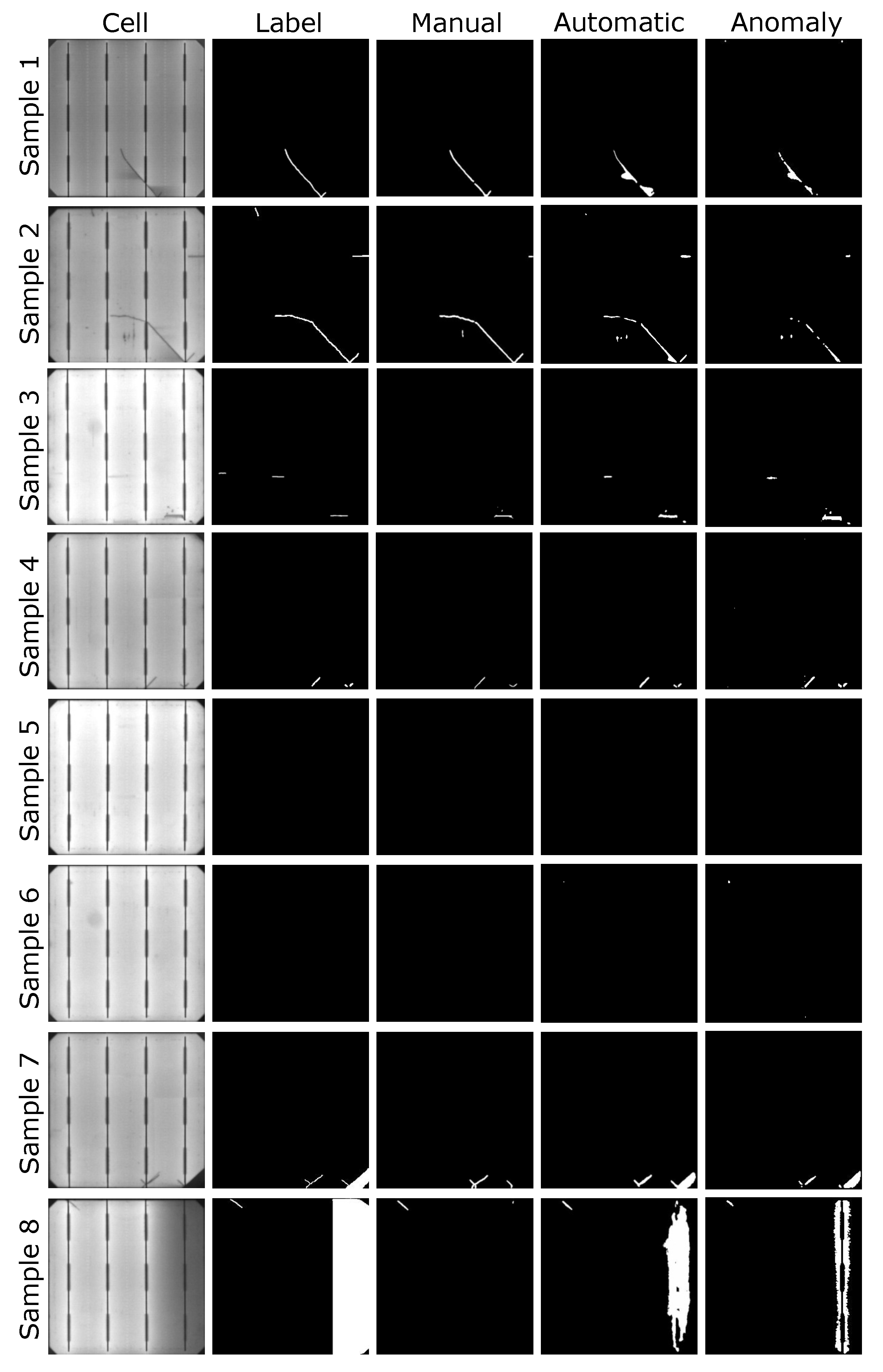
- Then, as defective cells arise, the anomaly detection model will separate them from the defect-free ones and it will generate pixel-level annotations without any human intervention. The experiments have shown that these segmentation results can be used as pixel-wise labels for the supervised training of a U-Net [44]-based model that improves the defect detection rates of the anomaly detection model.
3. Methodology
3.1. Unsupervised Model for Anomaly Detection
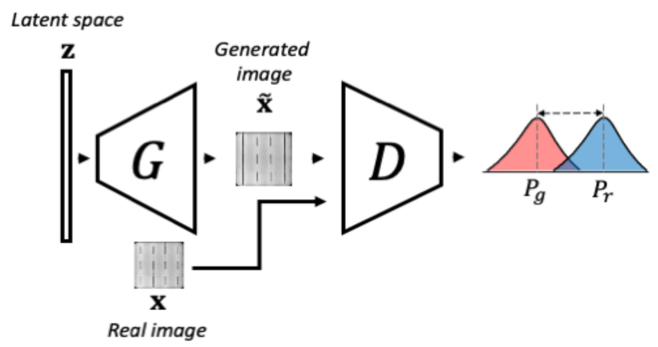
3.1.1. Phase 1-WGAN Training
3.1.2. Phase 2-Encoder Training
3.1.3. Anomaly Detection
3.2. Supervised Model for Defect Segmentation
4. Experimental Setup
4.1. Dataset
4.2. Metrics
4.3. Hardware and Software
5. Experiments
5.1. Unsupervised Model for Anomaly Detection
5.1.1. Experimental Design
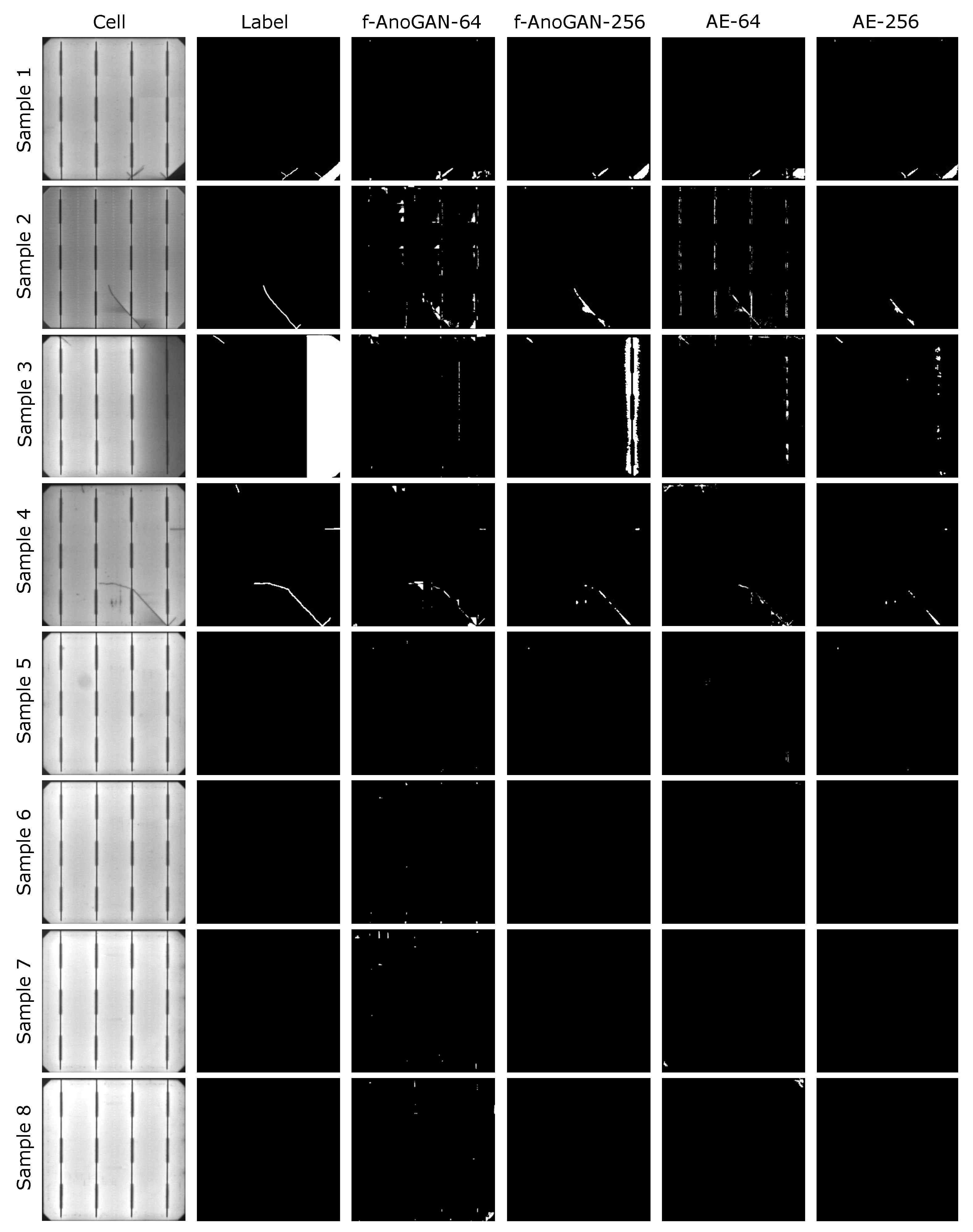
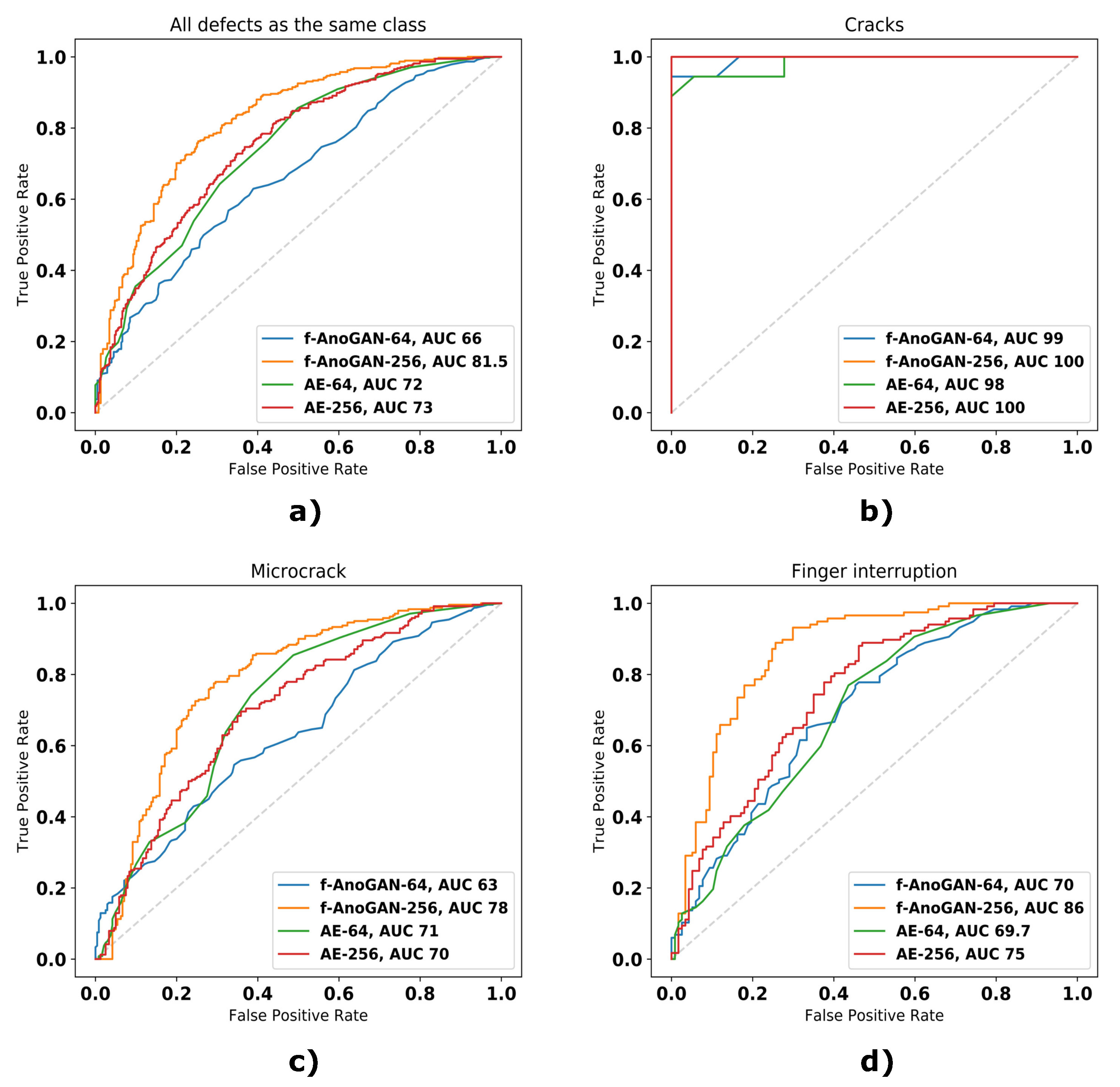
5.1.2. Results
5.2. Supervised Model for Defect Segmentation
5.2.1. Experimental Design
5.2.2. Results
6. Conclusions
Author Contributions
Funding
Institutional Review Board Statement
Informed Consent Statement
Acknowledgments
Conflicts of Interest
References
- Frankfurt School-UNEP Centre/BNEF. Global Trends in Renewable Energy. 2019. Available online: https://www.fs-unep-centre.org/wp-content/uploads/2019/11/GTR_2019.pdf (accessed on 24 April 2020).
- IEA. Renewables 2019. 2019. Available online: https://www.iea.org/reports/renewables-2019 (accessed on 24 April 2020).
- Köntges, M.; Kunze, I.; Kajari-Schröder, S.; Breitenmoser, X.; Bjørneklett, B. The risk of power loss in crystalline silicon based photovoltaic modules due to micro-cracks. Sol. Energy Mater. Sol. Cells 2011, 95, 1131–1137. [Google Scholar] [CrossRef]
- Bartler, A.; Mauch, L.; Yang, B.; Reuter, M.; Stoicescu, L. Automated Detection of Solar Cell Defects with Deep Learning. In Proceedings of the 26th European Signal Processing Conference, EUSIPCO 2018, Roma, Italy, 3–7 September 2018; pp. 2035–2039. [Google Scholar] [CrossRef]
- Chen, H.; Hu, Q.; Zhai, B.; Chen, H.; Liu, K. A robust weakly supervised learning of deep Conv-Nets for surface defect inspection. Neural Comput. Appl. 2020, 32, 11229–11244. [Google Scholar] [CrossRef]
- Demant, M.; Rein, S.; Haunschild, J.; Strauch, T.; Hoffler, H.; Broisch, J.; Wasmer, S.; Sunder, K.; Anspach, O.; Brox, T. Inline quality rating of multi-crystalline wafers based on photoluminescence images. Prog. Photovoltaics Res. Appl. 2016, 24, 1533–1546. [Google Scholar] [CrossRef]
- Nos, O.; Favre, W.; Jay, F.; Ozanne, F.; Valla, A.; Alvarez, J.; Muñoz, D.; Ribeyron, P. Quality control method based on photoluminescence imaging for the performance prediction of c-Si/a-Si: H heterojunction solar cells in industrial production lines. Sol. Energy Mater. Sol. Cells 2016, 144, 210–220. [Google Scholar] [CrossRef]
- Pierdicca, R.; Malinverni, E.; Piccinini, F.; Paolanti, M.; Felicetti, A.; Zingaretti, P. Deep Concolutional Neural Network for automatic detection of damaged photovoltaic cells. In Proceedings of the ISPRS TC II Mid-term Symposium “Towards Photogrammetry 2020”, Riva del Garda, Italy, 4–7 June 2018. [Google Scholar] [CrossRef] [Green Version]
- Vaněk, J.; Repko, I.; Klima, J. Automation capabilities of solar modules defect detection by thermography. ECS Trans. 2016, 74, 293–303. [Google Scholar] [CrossRef]
- Fuyuki, T.; Kitiyanan, A. Photographic diagnosis of crystalline silicon solar cells utilizing electroluminescence. Appl. Phys. A 2009, 96, 189–196. [Google Scholar] [CrossRef]
- Tang, W.; Yang, Q.; Xiong, K.; Yan, W. Deep learning based automatic defect identification of photovoltaic module using electroluminescence images. Sol. Energy 2020, 201, 453–460. [Google Scholar] [CrossRef]
- Ko, J.; Rheem, J. Anisotropic diffusion based micro-crack inspection in polycrystalline solar wafers. In Proceedings of the World Congress on Engineering 2012, International Association of Engineers, London, UK, 4–6 July 2012; Volume 2188, pp. 524–528. [Google Scholar]
- Anwar, S.A.; Abdullah, M.Z. Micro-crack detection of multicrystalline solar cells featuring an improved anisotropic diffusion filter and image segmentation technique. EURASIP J. Image Video Process. 2014, 2014, 15. [Google Scholar] [CrossRef] [Green Version]
- Chen, H.; Zhao, H.; Han, D.; Liu, K. Accurate and robust crack detection using steerable evidence filtering in electroluminescence images of solar cells. Opt. Lasers Eng. 2019, 118, 22–33. [Google Scholar] [CrossRef]
- Chen, H.; Zhao, H.; Han, D.; Yan, H.; Zhang, X.; Liu, K. Robust Crack Defect Detection in Inhomogeneously Textured Surface of Near Infrared Images. In Proceedings of the Chinese Conference on Pattern Recognition and Computer Vision (PRCV), Guangzhou, China, 23–26 November 2018; Springer: Berlin/Heidelberg, Germany, 2018; pp. 511–523. [Google Scholar] [CrossRef]
- Tsai, D.M.; Chang, C.C.; Chao, S.M. Micro-crack inspection in heterogeneously textured solar wafers using anisotropic diffusion. Image Vis. Comput. 2010, 28, 491–501. [Google Scholar] [CrossRef]
- Tsai, D.M.; Wu, S.C.; Li, W.C. Defect detection of solar cells in electroluminescence images using Fourier image reconstruction. Sol. Energy Mater. Sol. Cells 2012, 99, 250–262. [Google Scholar] [CrossRef]
- Tsai, D.; Wu, S.; Chiu, W. Defect Detection in Solar Modules Using ICA Basis Images. IEEE Trans. Ind. Informatics 2013, 9, 122–131. [Google Scholar] [CrossRef]
- Zhang, X.; Sun, H.; Zhou, Y.; Xi, J.; Li, M. A Novel Method for Surface Defect Detection of Photovoltaic Module Based on Independent Component Analysis. Math. Probl. Eng. 2013, 2013, 520568. [Google Scholar] [CrossRef]
- Rodriguez, A.; Gonzalez, C.; Fernandez, A.; Rodriguez, F.; Delgado, T.; Bellman, M. Automatic solar cell diagnosis and treatment. J. Intell. Manuf. 2021, 32, 1163–1172. [Google Scholar] [CrossRef]
- Tsai, D.M.; Li, G.N.; Li, W.C.; Chiu, W.Y. Defect detection in multi-crystal solar cells using clustering with uniformity measures. Adv. Eng. Informatics 2015, 29, 419–430. [Google Scholar] [CrossRef]
- Su, B.; Chen, H.; Zhu, Y.; Liu, W.; Liu, K. Classification of Manufacturing Defects in Multicrystalline Solar Cells With Novel Feature Descriptor. IEEE Trans. Instrum. Meas. 2019, 68, 4675–4688. [Google Scholar] [CrossRef]
- Akram, M.W.; Li, G.; Jin, Y.; Chen, X.; Zhu, C.; Zhao, X.; Khaliq, A.; Faheem, M.; Ahmad, A. CNN based automatic detection of photovoltaic cell defects in electroluminescence images. Energy 2019, 189, 116319. [Google Scholar] [CrossRef]
- Dunderdale, C.; Brettenny, W.; Clohessy, C.; van Dyk, E.E. Photovoltaic defect classification through thermal infrared imaging using a machine learning approach. Prog. Photovoltaics Res. Appl. 2020, 28, 177–188. [Google Scholar] [CrossRef]
- Deitsch, S.; Christlein, V.; Berger, S.; Buerhop-Lutz, C.; Maier, A.; Gallwitz, F.; Riess, C. Automatic classification of defective photovoltaic module cells in electroluminescence images. Sol. Energy 2019, 185, 455–468. [Google Scholar] [CrossRef] [Green Version]
- Akram, M.W.; Li, G.; Jin, Y.; Chen, X.; Zhu, C.; Ahmad, A. Automatic detection of photovoltaic module defects in infrared images with isolated and develop-model transfer deep learning. Sol. Energy 2020, 198, 175–186. [Google Scholar] [CrossRef]
- Chen, H.; Pang, Y.; Hu, Q.; Liu, K. Solar cell surface defect inspection based on multispectral convolutional neural network. J. Intell. Manuf. 2020, 31, 453–468. [Google Scholar] [CrossRef] [Green Version]
- Balzategui, J.; Eciolaza, L.; Arana-Arexolaleiba, N.; Altube, J.; Aguerre, J.; Legarda-Ereño, I.; Apraiz, A. Semi-automatic quality inspection of solar cell based on Convolutional Neural Networks. In Proceedings of the 2019 24th IEEE International Conference on Emerging Technologies and Factory Automation (ETFA), Zaragoza, Spain, 10–13 September 2019; pp. 529–535. [Google Scholar] [CrossRef]
- Balzategui, J.; Eciolaza, L.; Arana-Arexolaleiba, N. Defect detection on Polycrystalline solar cells using Electroluminescence and Fully Convolutional Neural Networks. In Proceedings of the 2020 IEEE/SICE International Symposium on System Integration (SII), Honolulu, HI, USA, 12–15 January 2020; pp. 949–953. [Google Scholar] [CrossRef]
- Liu, L.; Zhu, Y.; Rahman, M.R.U.; Zhao, P.; Chen, H. Surface Defect Detection of Solar Cells Based on Feature Pyramid Network and GA-Faster-RCNN. In Proceedings of the 2019 2nd China Symposium on Cognitive Computing and Hybrid Intelligence (CCHI), Xi’an, China, 21–22 September 2019; pp. 292–297. [Google Scholar] [CrossRef]
- Zhang, X.; Hao, Y.; Shangguan, H.; Zhang, P.; Wang, A. Detection of surface defects on solar cells by fusing Multi-channel convolution neural networks. Infrared Phys. Technol. 2020, 108, 103334. [Google Scholar] [CrossRef]
- Mayr, M.; Hoffmann, M.; Maier, A.; Christlein, V. Weakly Supervised Segmentation of Cracks on Solar Cells Using Normalized Lp Norm. In Proceedings of the 2019 IEEE International Conference on Image Processing (ICIP), Taipei, Taiwan, 22–25 September 2019; pp. 1885–1889. [Google Scholar] [CrossRef] [Green Version]
- Demirci, M.; Beşli, N.; Gümüşçü, A. Defective PV Cell Detection Using Deep Transfer Learning and EL Imaging. In Proceedings of the International Conference on Data Science, Machine Learning and Statistics 2019 (DMS-2019), Istanbul, Turkey, 26–29 June 2019; p. 311. [Google Scholar]
- Qian, X.; Li, J.; Cao, J.; Wu, Y.; Wang, W. Micro-cracks detection of solar cells surface via combining short-term and long-term deep features. Neural Networks Off. J. Int. Neural Netw. Soc. 2020, 127, 132–140. [Google Scholar] [CrossRef]
- Goodfellow, I.; Pouget-Abadie, J.; Mirza, M.; Xu, B.; Warde-Farley, D.; Ozair, S.; Courville, A.; Bengio, Y. Generative Adversarial Nets. In NIPS’14: Proceedings of the 27th International Conference on Neural Information Processing Systems; MIT Press: Cambridge, MA, USA, 2014; Volume 2, pp. 2672–2680. [Google Scholar]
- Choi, Y.; Choi, M.; Kim, M.; Ha, J.W.; Kim, S.; Choo, J. StarGAN: Unified Generative Adversarial Networks for Multi-domain Image-to-Image Translation. In Proceedings of the 2018 IEEE/CVF Conference on Computer Vision and Pattern Recognition, Salt Lake City, UT, USA, 18–22 June 2018; pp. 8789–8797. [Google Scholar] [CrossRef] [Green Version]
- Zhang, W.; Li, X.; Jia, X.D.; Ma, H.; Luo, Z.; Li, X. Machinery fault diagnosis with imbalanced data using deep generative adversarial networks. Measurement 2020, 152, 107377. [Google Scholar] [CrossRef]
- Luo, Z.; Cheng, S.; Zheng, Q. GAN-Based Augmentation for Improving CNN Performance of Classification of Defective Photovoltaic Module Cells in Electroluminescence Images. In Proceedings of the IOP Conference Series: Earth and Environmental Science, Macao, China, 21–24 July 2019; IOP Publishing: Bristol, UK, 2019; Volume 354, p. 012106. [Google Scholar] [CrossRef] [Green Version]
- Haselmann, M.; Gruber, D.P.; Tabatabai, P. Anomaly detection using deep learning based image completion. In Proceedings of the 2018 17th IEEE International Conference on Machine Learning and Applications (ICMLA), Orlando, FL, USA, 17–20 December 2018; pp. 1237–1242. [Google Scholar] [CrossRef] [Green Version]
- Staar, B.; Lütjen, M.; Freitag, M. Anomaly detection with convolutional neural networks for industrial surface inspection. Procedia CIRP 2019, 79, 484–489. [Google Scholar] [CrossRef]
- Schlegl, T.; Seeböck, P.; Waldstein, S.M.; Langs, G.; Schmidt-Erfurth, U. f-AnoGAN: Fast unsupervised anomaly detection with generative adversarial networks. Med. Image Anal. 2019, 54, 30–44. [Google Scholar] [CrossRef]
- Chen, X.; Konukoglu, E. Unsupervised Detection of Lesions in Brain MRI using Constrained Adversarial Auto-encoders. In Proceedings of the MIDL Conference Book, Amsterdam, The Netherlands, 4–6 July 2018; MIDL: Amsterdam, The Netherlands, 2018. [Google Scholar] [CrossRef]
- Qian, X.; Li, J.; Zhang, J.; Zhang, W.; Yue, W.; Wu, Q.E.; Zhang, H.; Wu, Y.; Wang, W. Micro-crack detection of solar cell based on adaptive deep features and visual saliency. Sens. Rev. 2020, 40, 385–396. [Google Scholar] [CrossRef]
- Ronneberger, O.; Fischer, P.; Brox, T. U-Net: Convolutional Networks for Biomedical Image Segmentation. In Medical Image Computing and Computer-Assisted Intervention–MICCAI 2015; Springer: Cham, Switzerland, 2015; pp. 234–241. [Google Scholar] [CrossRef] [Green Version]
- Gulrajani, I.; Ahmed, F.; Arjovsky, M.; Dumoulin, V.; Courville, A. Improved Training of Wasserstein GANs. In Proceedings of the 31st International Conference on Neural Information Processing Systems; Curran Associates Inc.: Red Hook, NY, USA, 2017; pp. 5769–5779. [Google Scholar]
- Kignma, D.P.; Ba, J. Adam: A method for stochastic optimization. arxiv 2014, arXiv:1412.6980. [Google Scholar]
- Hinton, G.; Srivastava, N.; Swersky, K. Neural Networks for Machine Learning Lecture 6a Overview of Mini-Batch Gradient Descent. 2012. Available online: https://www.cs.toronto.edu/~hinton/coursera/lecture6/lec6.pdf (accessed on 28 April 2020).
- Chintala, S.; Denton, E.; Arjovsky, M.; Mathieu, M. How to Train a GAN? Tips and Tricks to Make GANs Work. 2016. Available online: https://github.com/soumith/ganhacks (accessed on 5 June 2021).


| Total | ||
|---|---|---|
| Defect-free | 1498 | |
| Defective | 375 | |
| Crack | 18 | |
| Microcrack | 240 | |
| Finger interruptions | 117 | |
| Train | Val | Test | Total | ||
|---|---|---|---|---|---|
| Defect-free | 750 | 373 | 375 | 1498 | |
| Defective | - | - | 375 | 375 | |
| Crack | - | - | 18 | - | |
| Microcrack | - | - | 240 | - | |
| Finger interruptions | - | - | 117 | - | |
| Model | AUC | Precision | Recall | Specificity | f1-Score | |
|---|---|---|---|---|---|---|
| All test samples | ||||||
| f-AnoGAN-64 | 66 | 61.3 | 62.8 | 61 | 62 | |
| f-AnoGAN-256 | 81.5 | 75 | 78 | 75 | 77 | |
| AE-64 | 72 | 65.6 | 64 | 68 | 65 | |
| AE-256 | 73 | 68.4 | 58 | 72 | 63 | |
| Cracks | ||||||
| f-AnoGAN-64 | 99 | 66.7 | 100 | 50 | 80 | |
| f-AnoGAN-256 | 100 | 95 | 100 | 94 | 97 | |
| AE-64 | 98 | 78 | 100 | 100 | 87.7 | |
| AE-256 | 100 | 95 | 100 | 94 | 97 | |
| Micro | ||||||
| f-AnoGAN-64 | 63 | 58.7 | 59 | 59 | 58.9 | |
| f-AnoGAN-256 | 78 | 73 | 73 | 74 | 73 | |
| AE-64 | 71 | 66.5 | 63.7 | 67.9 | 65 | |
| AE-256 | 70 | 66 | 53 | 72 | 59 | |
| Finger int. | ||||||
| f-AnoGAN-64 | 70 | 66 | 64.9 | 66.7 | 65.5 | |
| f-AnoGAN-256 | 86 | 78 | 85 | 75 | 81 | |
| AE-64 | 69.7 | 61.9 | 59.8 | 63 | 60.8 | |
| AE-256 | 75 | 69 | 63 | 71 | 66 |
| Model | Time per Patch | Time per Image |
|---|---|---|
| f-AnoGAN-64 | 0.02 s | 5.12 s |
| f-AnoGAN-256 | - | 0.05 s |
| AE-64 | 0.012 s | 3.07 s |
| AE-256 | - | 0.02 s |
| Train | Val | Test | Total | ||
|---|---|---|---|---|---|
| Defect-free | - | - | 375 | 375 | |
| Defective | 232 | 68 | 75 | 375 | |
| Crack | 14 | 4 | 4 | 18 | |
| Microcrack | 152 | 50 | 48 | 240 | |
| Finger interruptions | 70 | 24 | 23 | 117 | |
| Model | Recall | Precision | Specificity |
|---|---|---|---|
| U-net w/ manual labels | 80 | 95 | 99 |
| U-net w/ auto. labels | 93 | 81 | 95 |
| f-AnoGAN-256 | 79 | 73 | 73 |
Publisher’s Note: MDPI stays neutral with regard to jurisdictional claims in published maps and institutional affiliations. |
© 2021 by the authors. Licensee MDPI, Basel, Switzerland. This article is an open access article distributed under the terms and conditions of the Creative Commons Attribution (CC BY) license (https://creativecommons.org/licenses/by/4.0/).
Share and Cite
Balzategui, J.; Eciolaza, L.; Maestro-Watson, D. Anomaly Detection and Automatic Labeling for Solar Cell Quality Inspection Based on Generative Adversarial Network. Sensors 2021, 21, 4361. https://doi.org/10.3390/s21134361
Balzategui J, Eciolaza L, Maestro-Watson D. Anomaly Detection and Automatic Labeling for Solar Cell Quality Inspection Based on Generative Adversarial Network. Sensors. 2021; 21(13):4361. https://doi.org/10.3390/s21134361
Chicago/Turabian StyleBalzategui, Julen, Luka Eciolaza, and Daniel Maestro-Watson. 2021. "Anomaly Detection and Automatic Labeling for Solar Cell Quality Inspection Based on Generative Adversarial Network" Sensors 21, no. 13: 4361. https://doi.org/10.3390/s21134361
APA StyleBalzategui, J., Eciolaza, L., & Maestro-Watson, D. (2021). Anomaly Detection and Automatic Labeling for Solar Cell Quality Inspection Based on Generative Adversarial Network. Sensors, 21(13), 4361. https://doi.org/10.3390/s21134361