Inductive Textile Sensor Design and Validation for a Wearable Monitoring Device


Abstract
1. Introduction
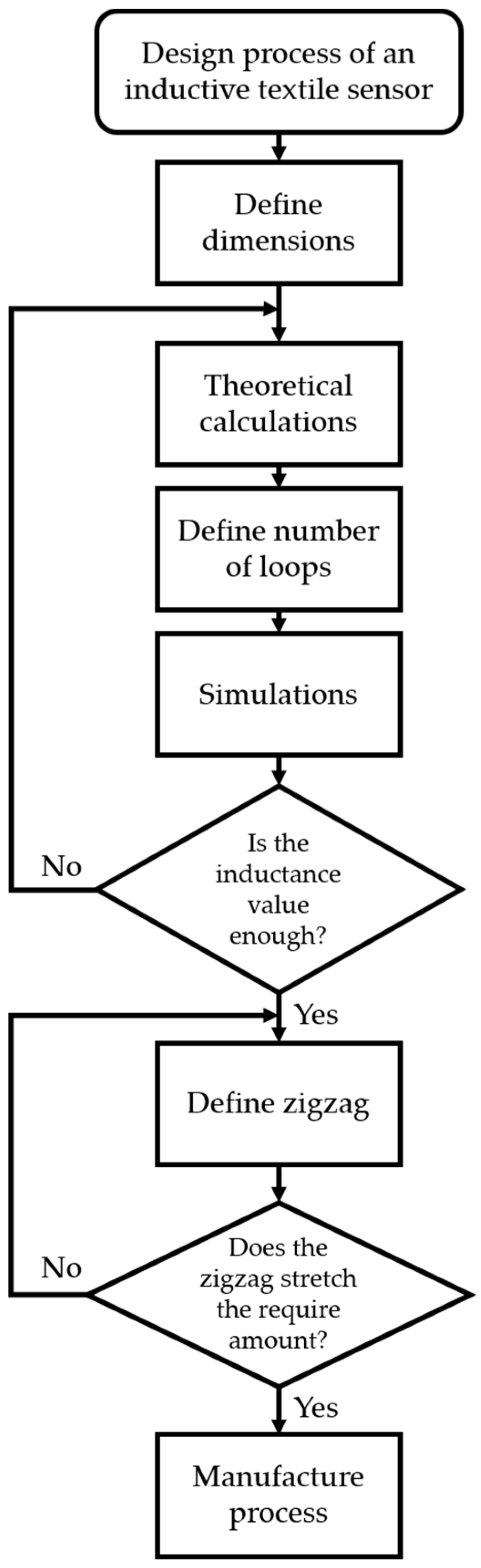
2. Design Process
2.1. Defining Maximum Size
2.2. Theoretical Calculation of the Inductance Value for a Flat Rectangular Coil Sensor
2.2.1. Inductance of a Rectangle with Round Wire
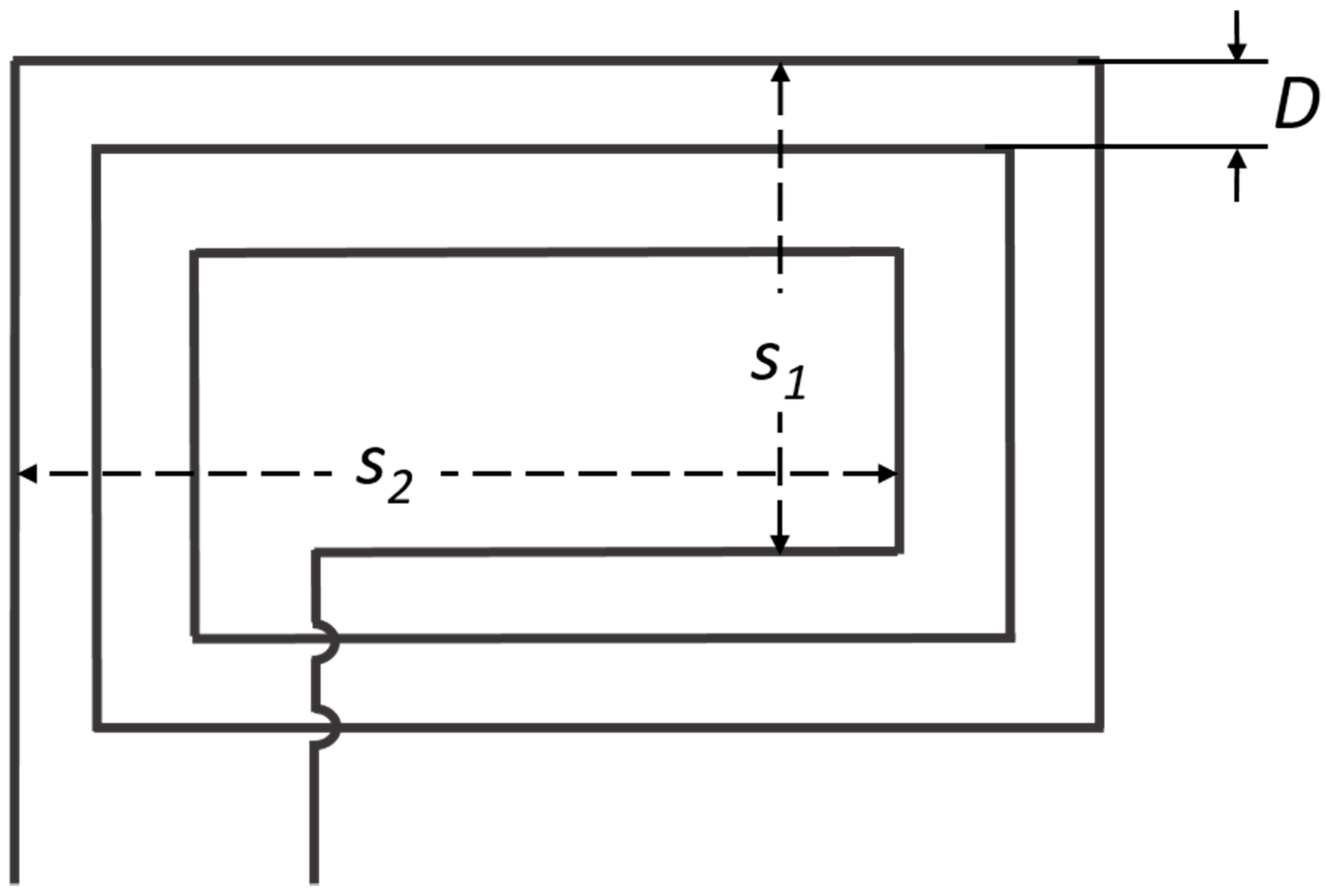
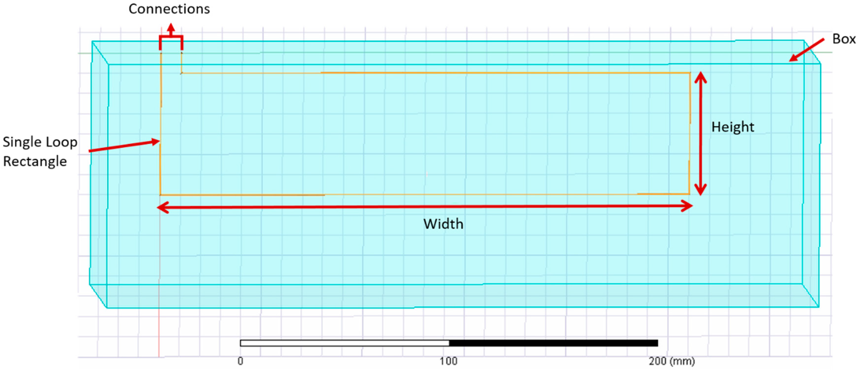
2.2.2. Flat Rectangular Coil
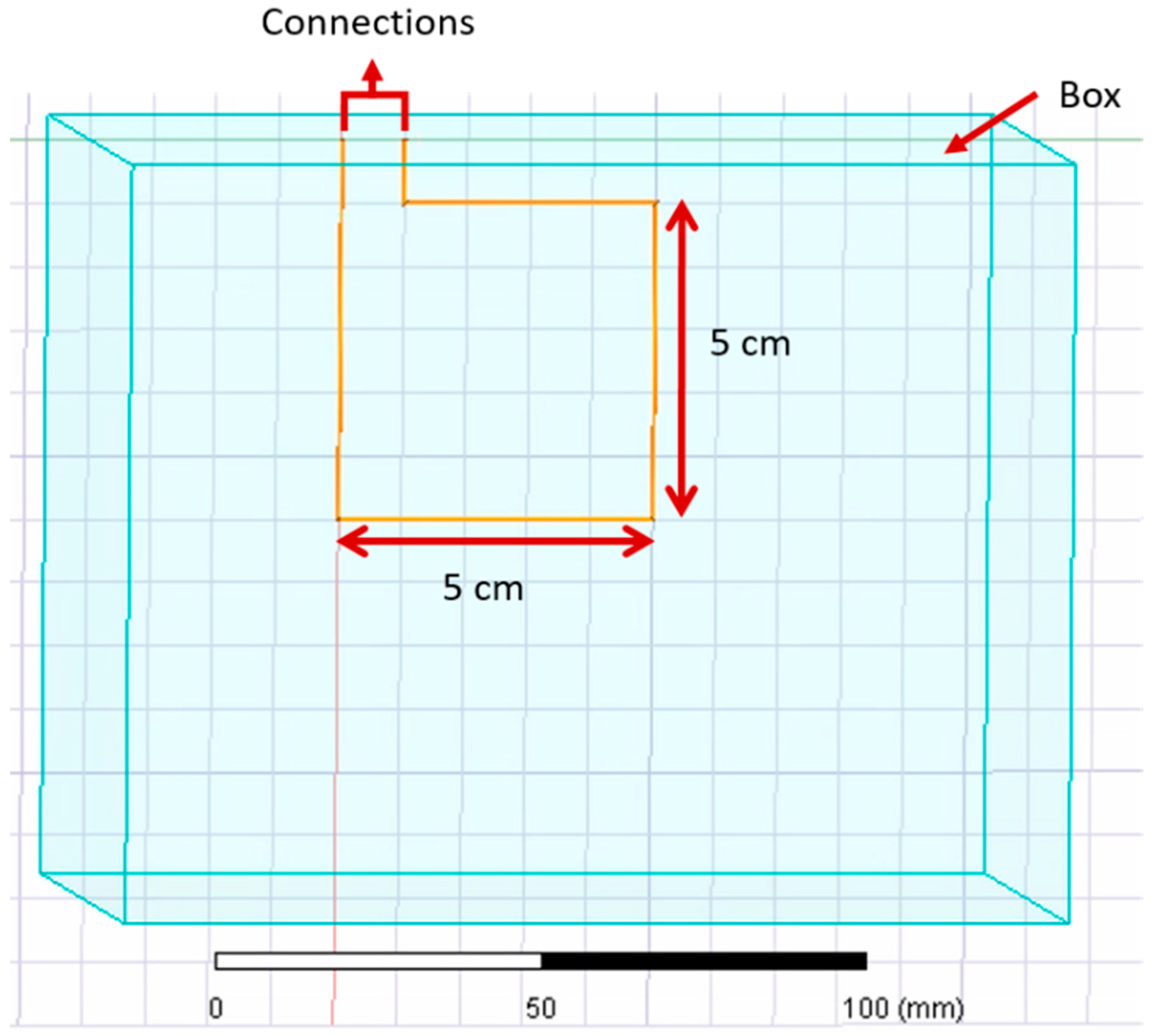
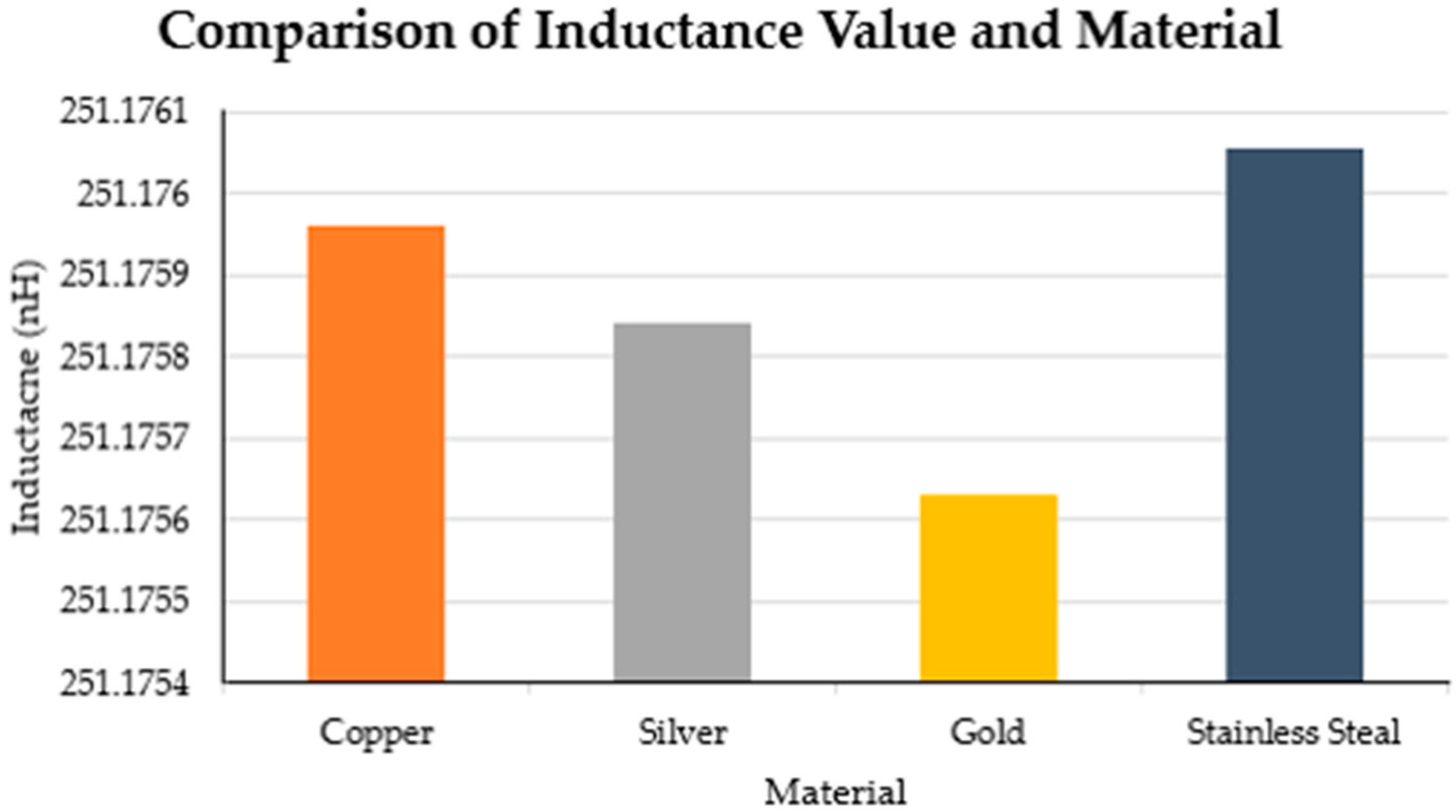
2.3. Simulations
2.4. Zigzag Properties
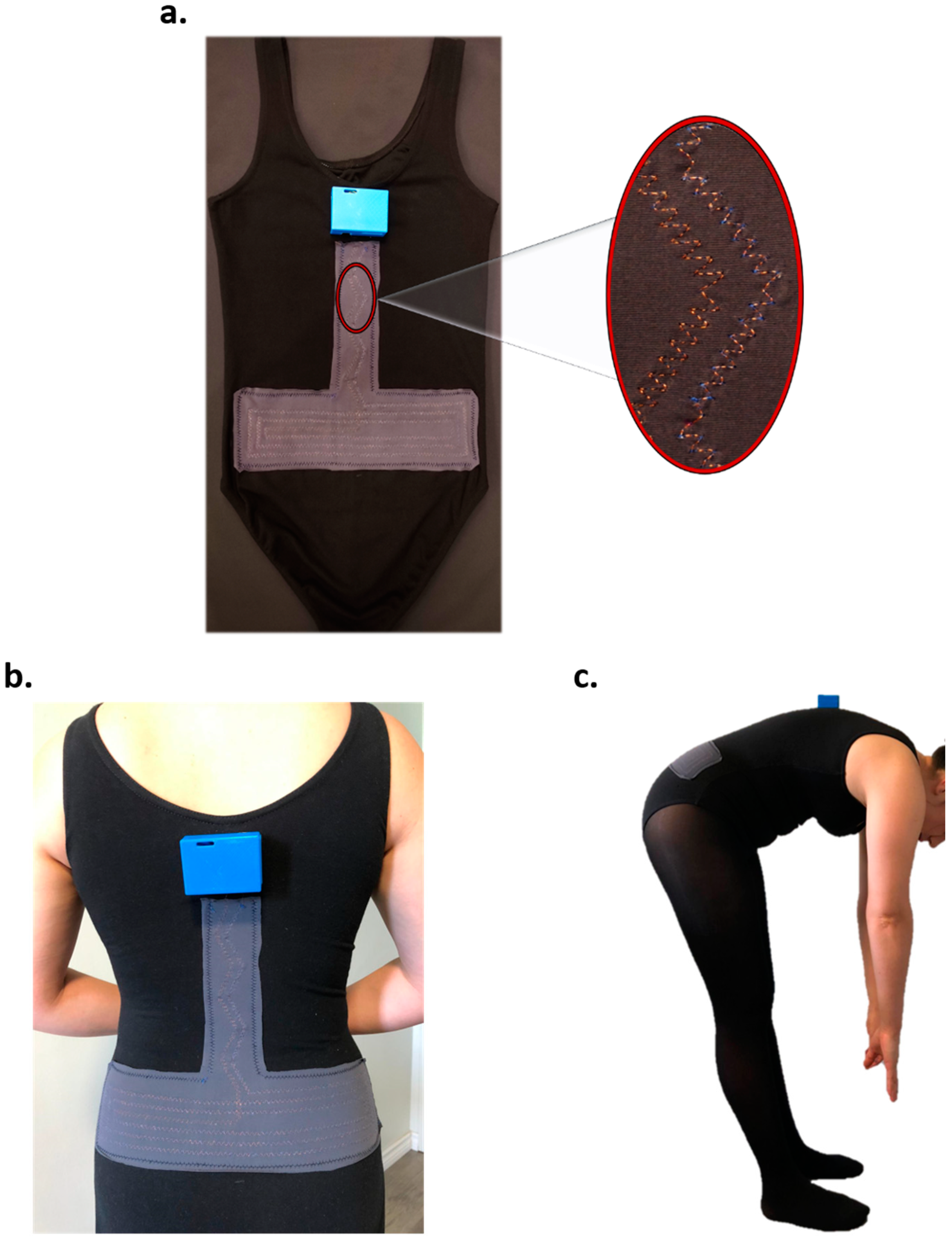
2.5. Manufacture Process
3. Example Case
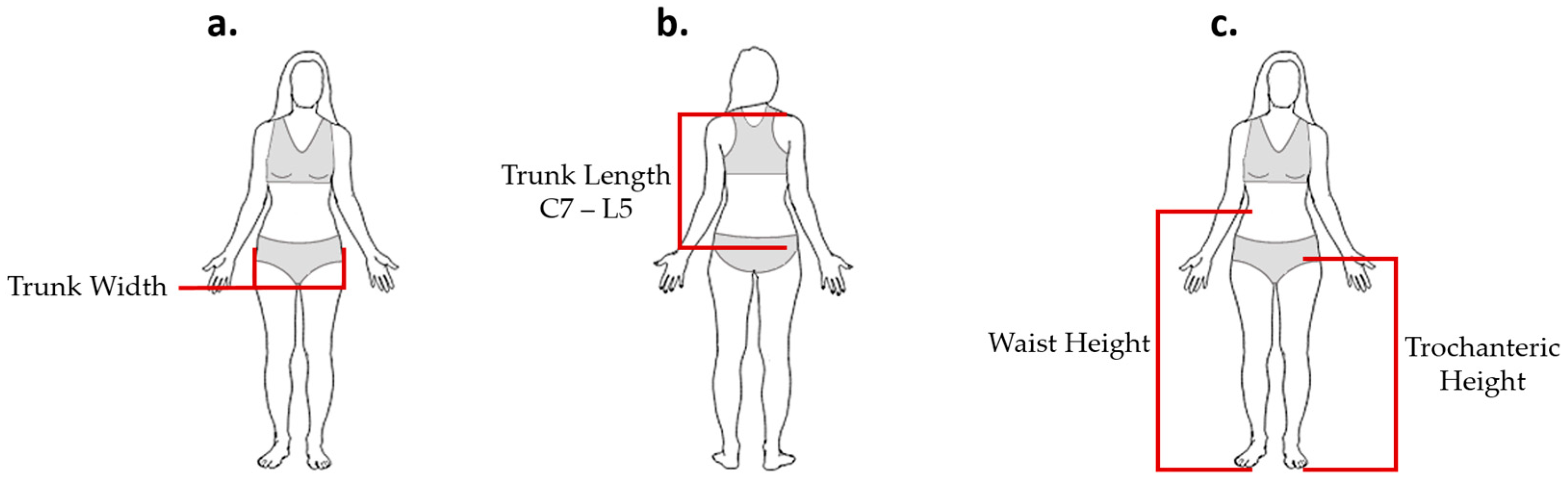
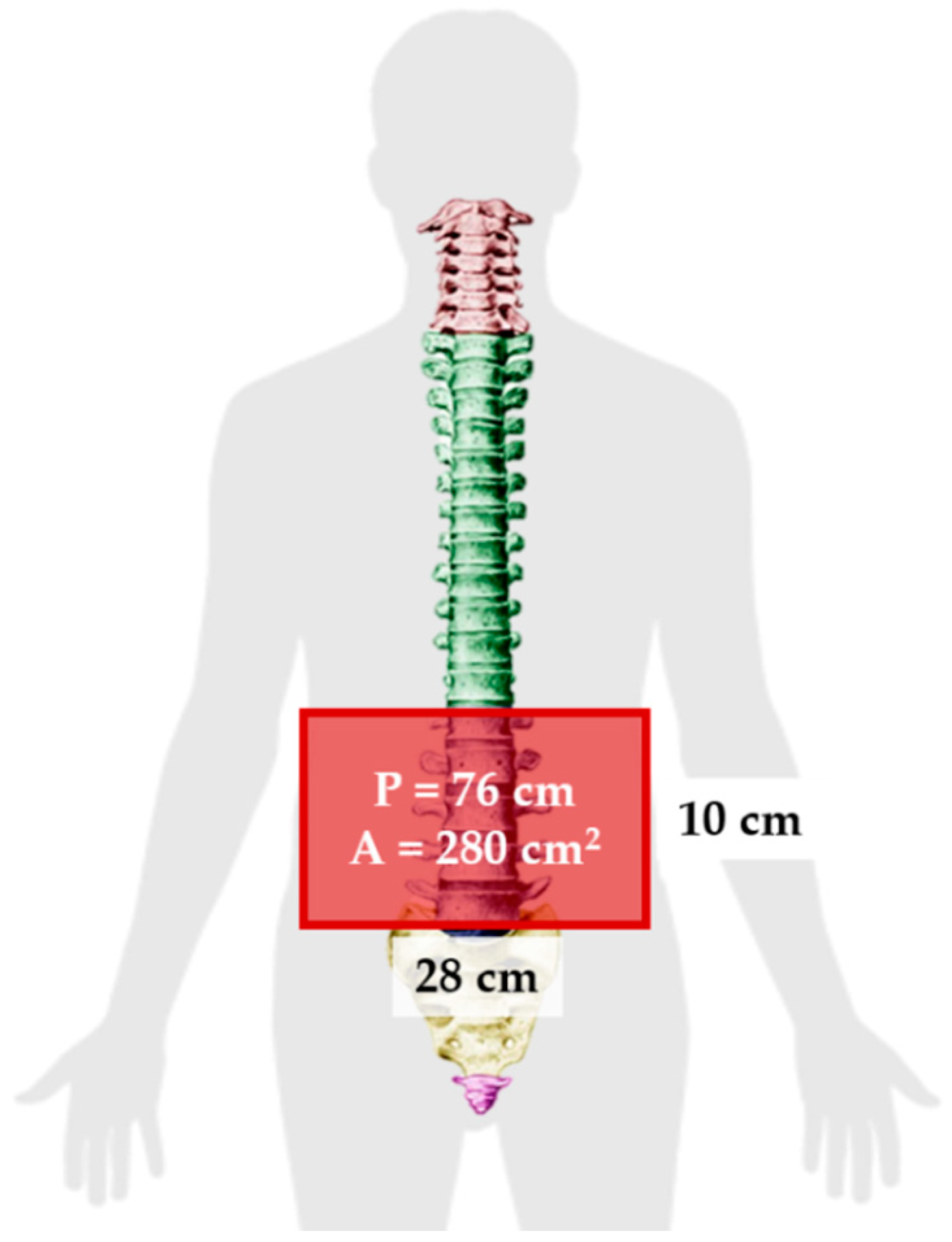
3.1. Anthropometry
3.2. Simulating Inductance Value of a Rectangle Using Ansys
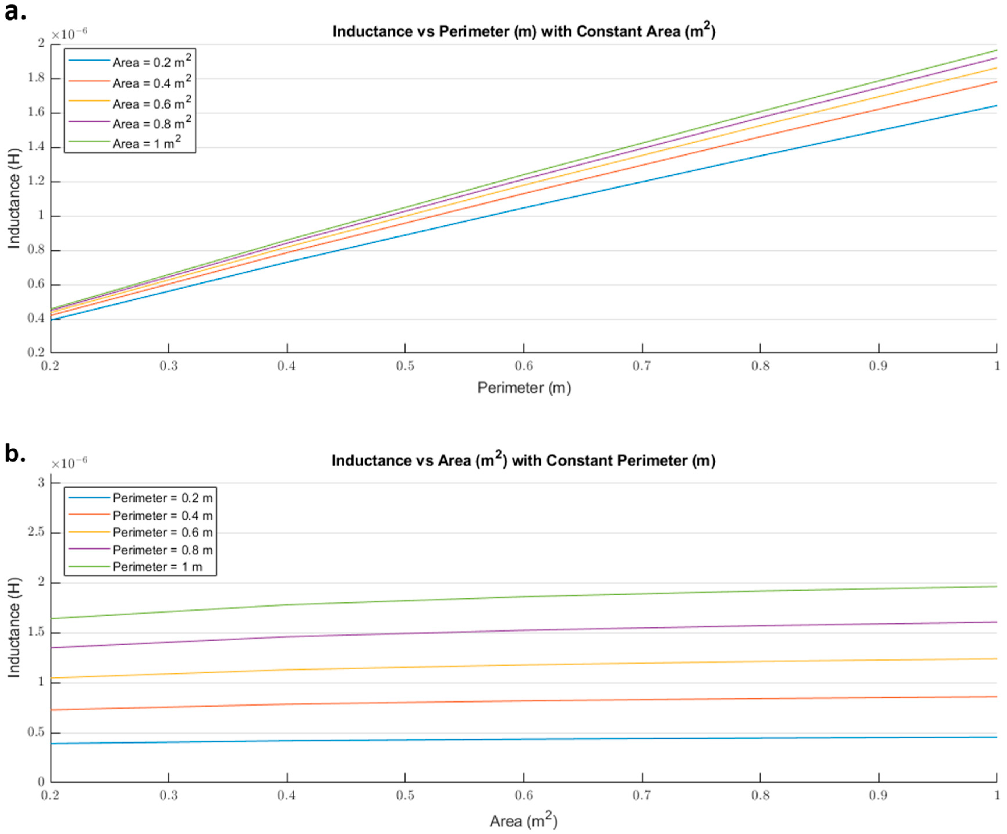
3.2.1. Inductance Change Based on Perimeter and Area
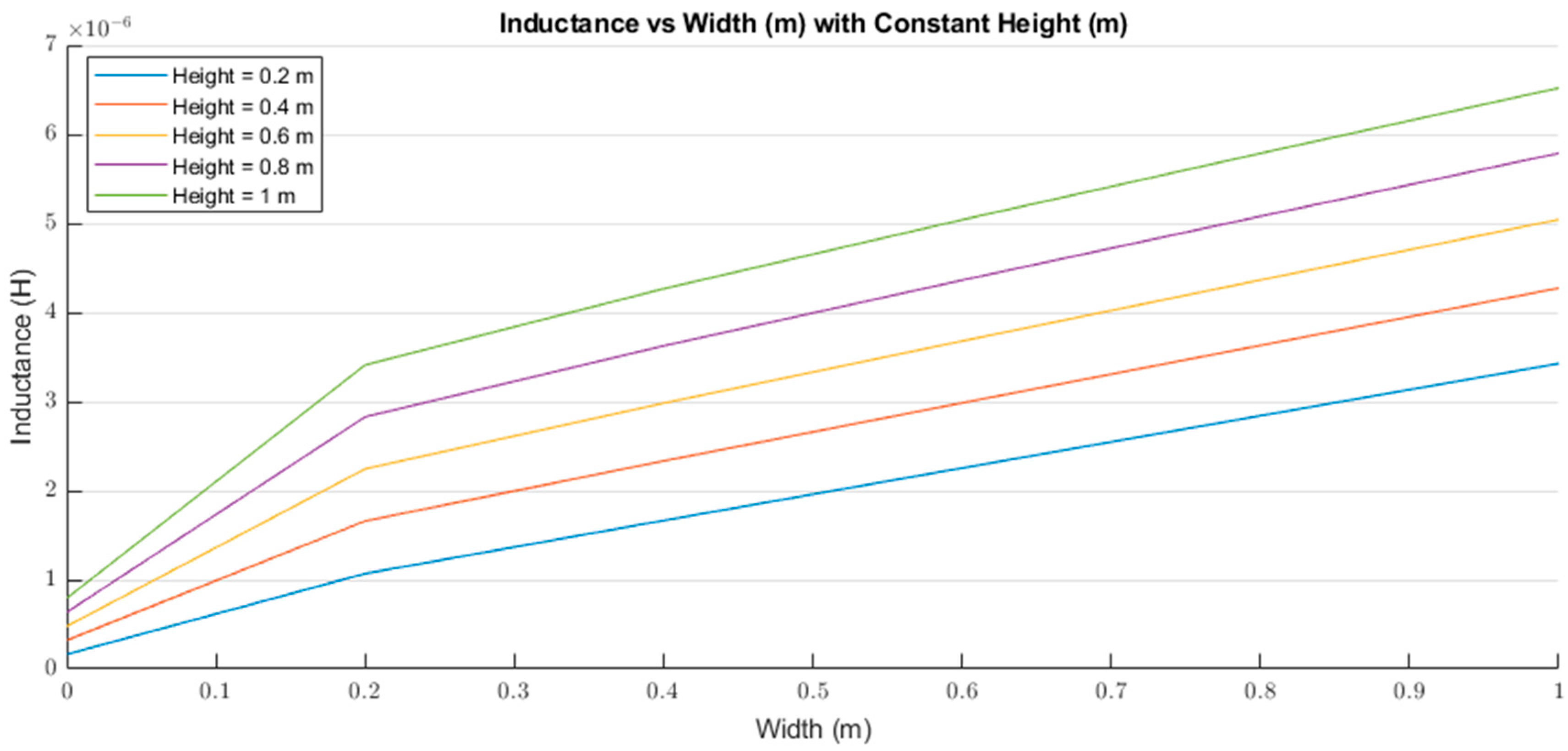
3.2.2. Inductance Change Based on Height and Width
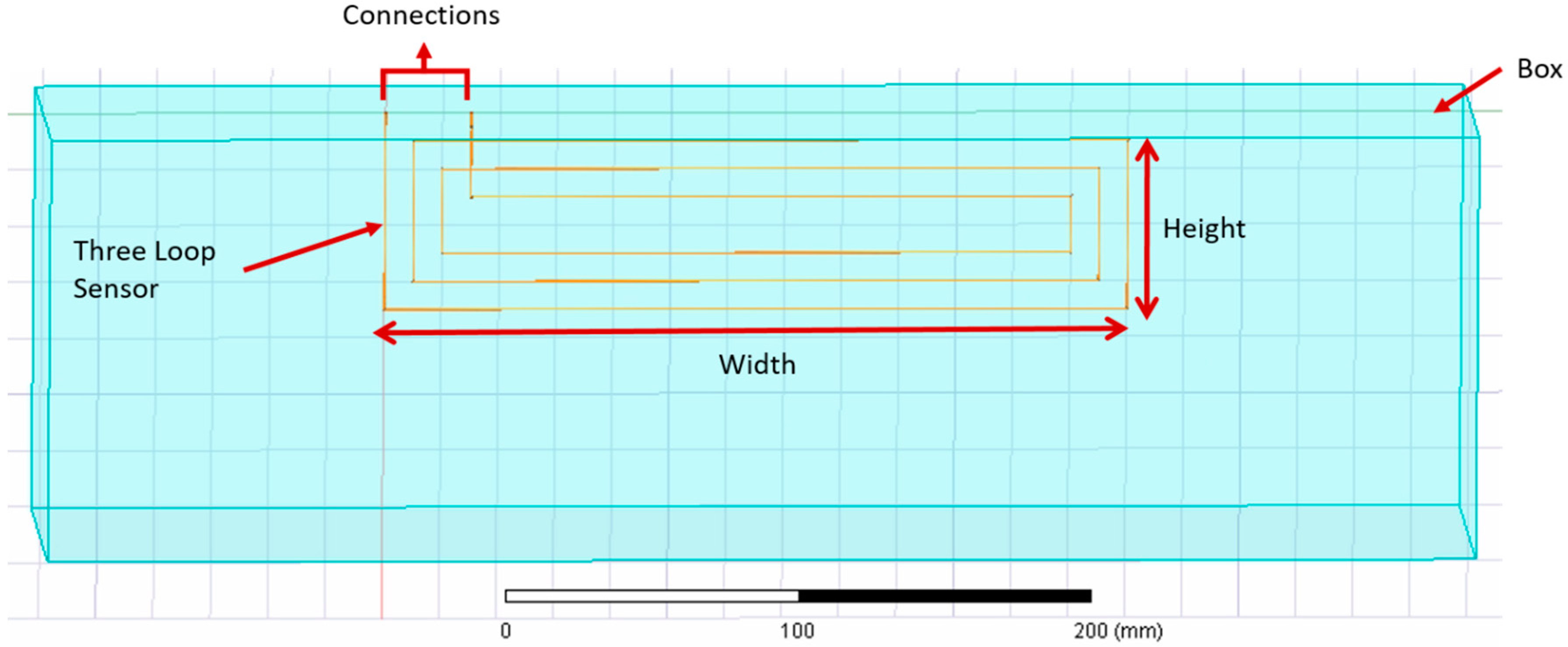
3.2.3. Inductance Change Based on the Number of Loops in a Flat Rectangular Coil
3.3. Results
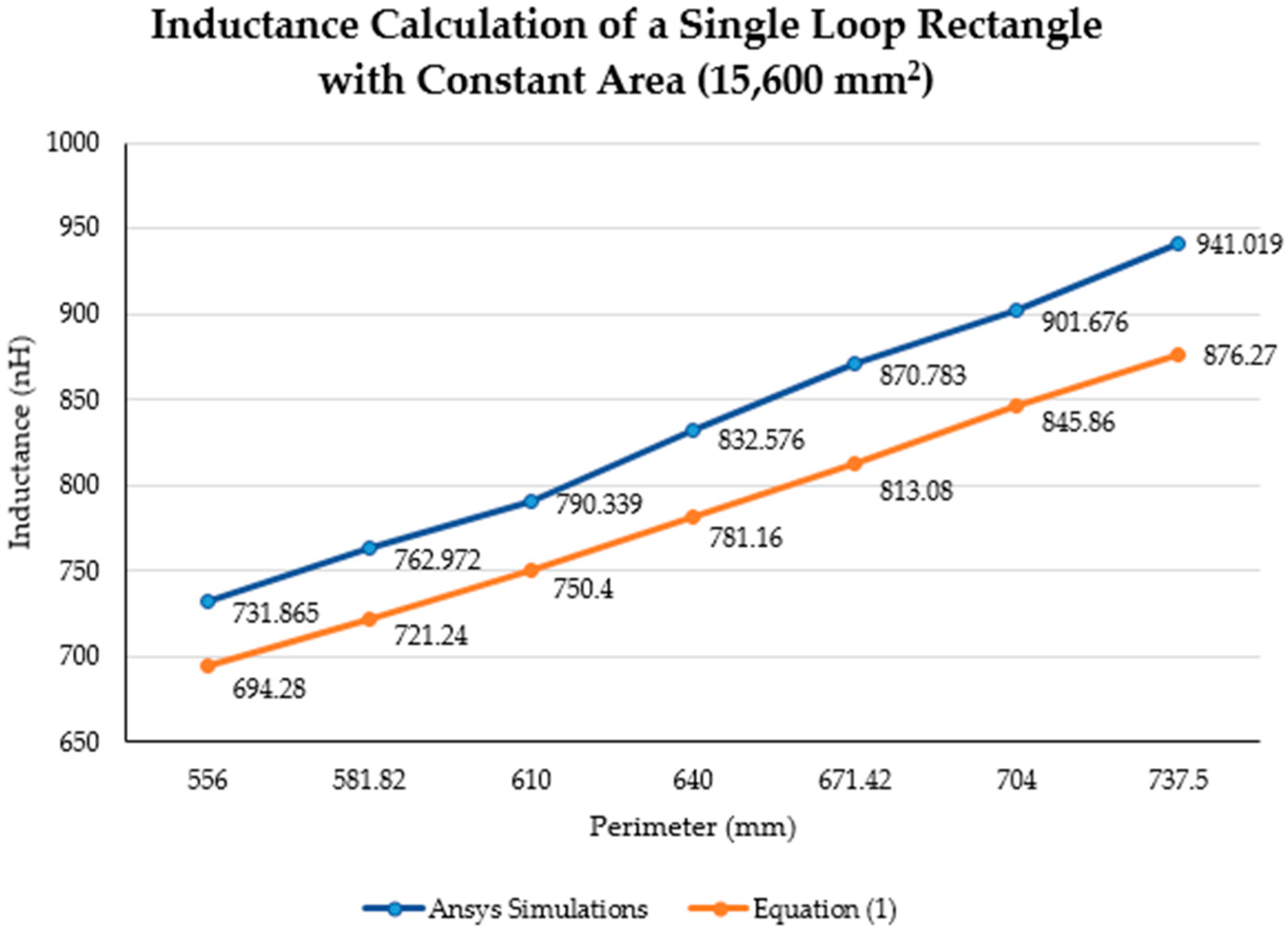
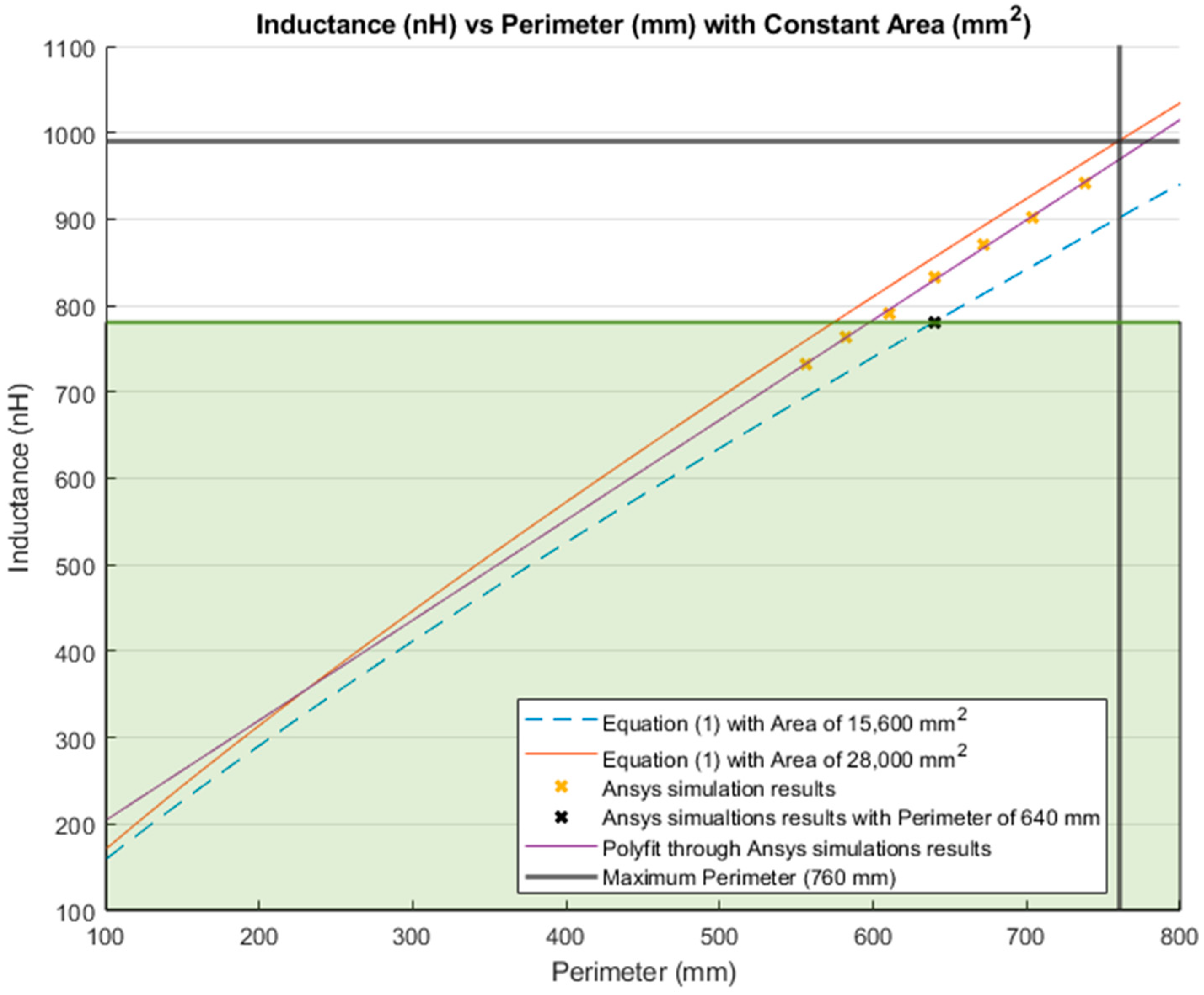
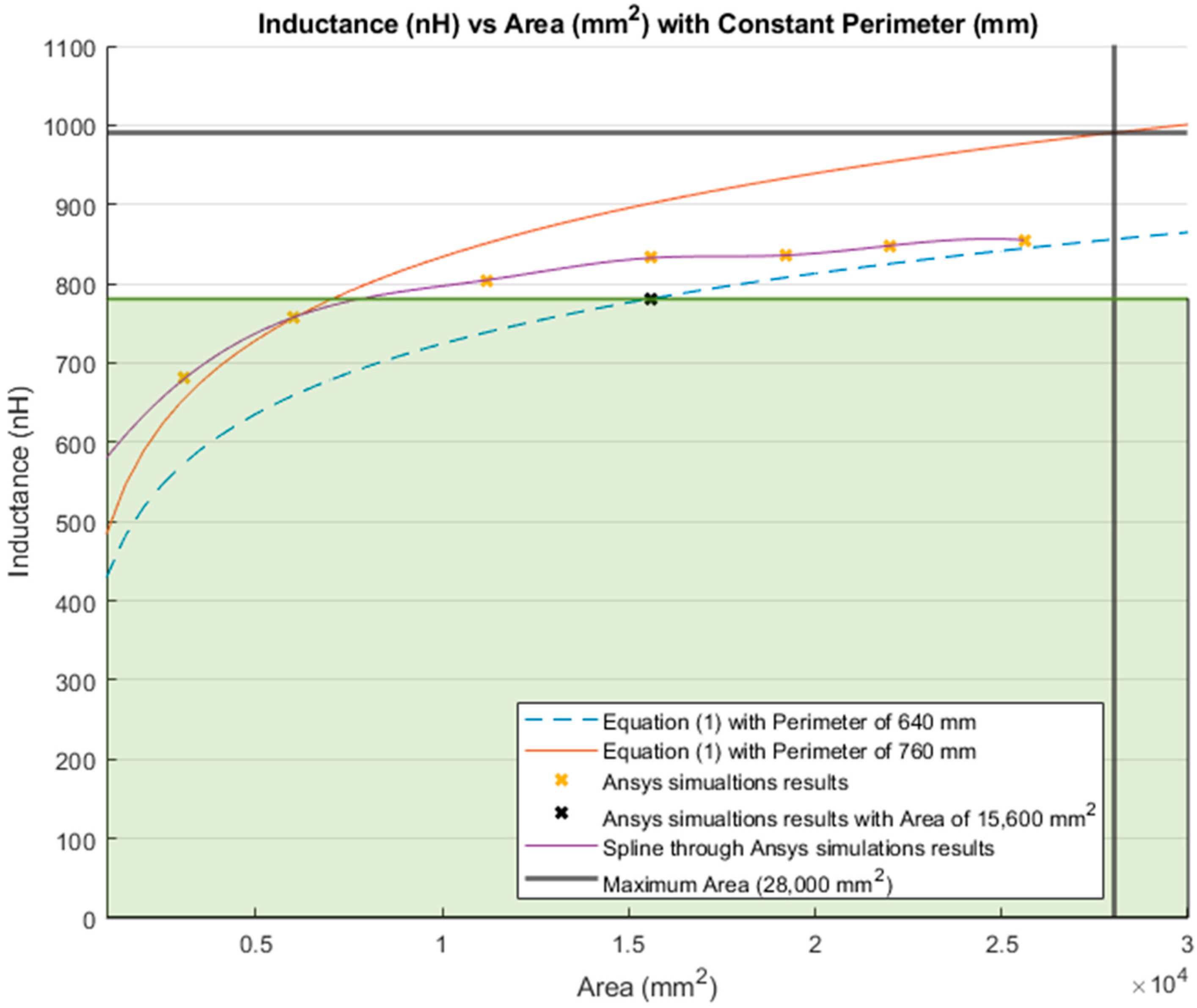
3.3.1. Comparison between Calculations and Simulations: Inductance Change Based on Perimeter and Area
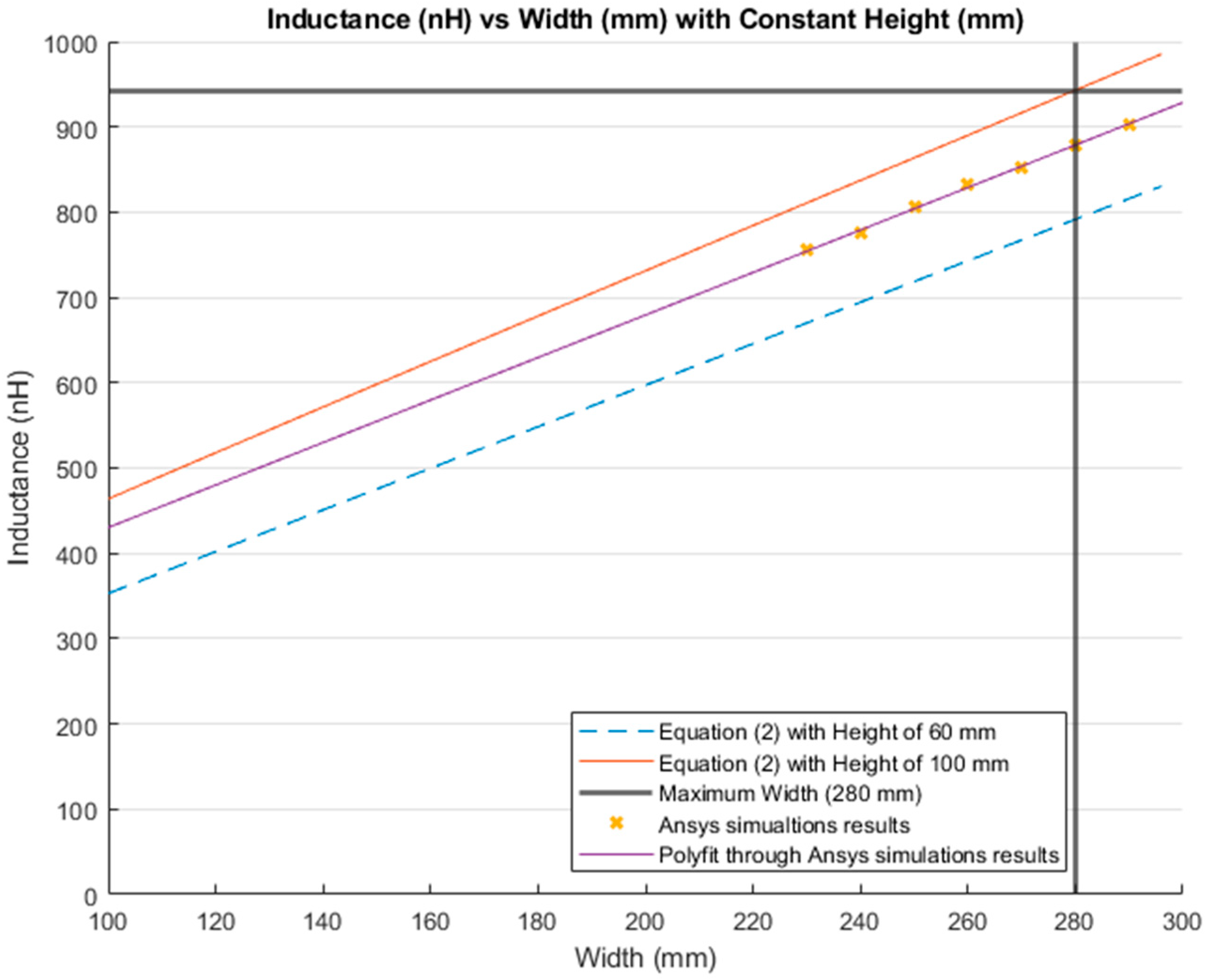
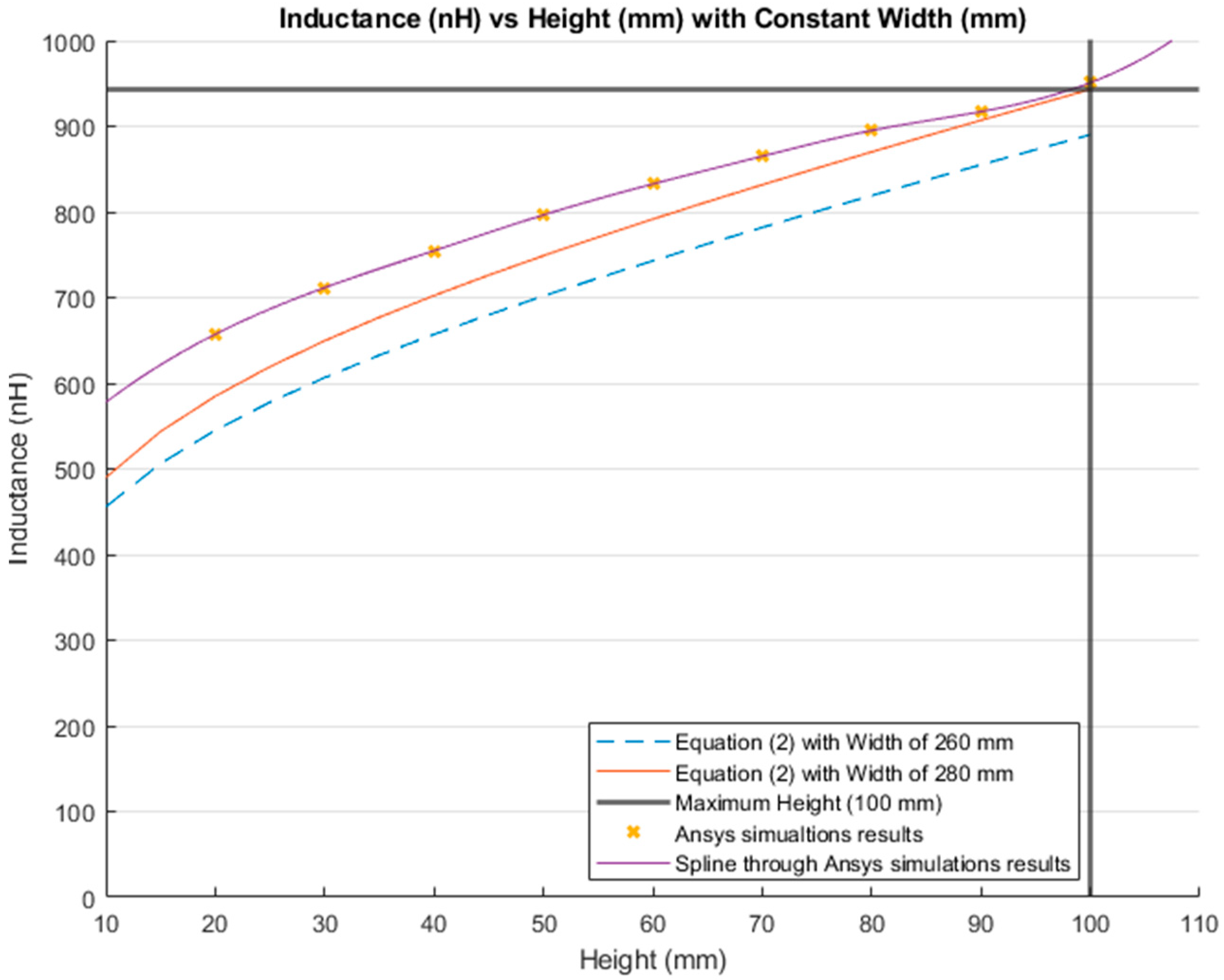
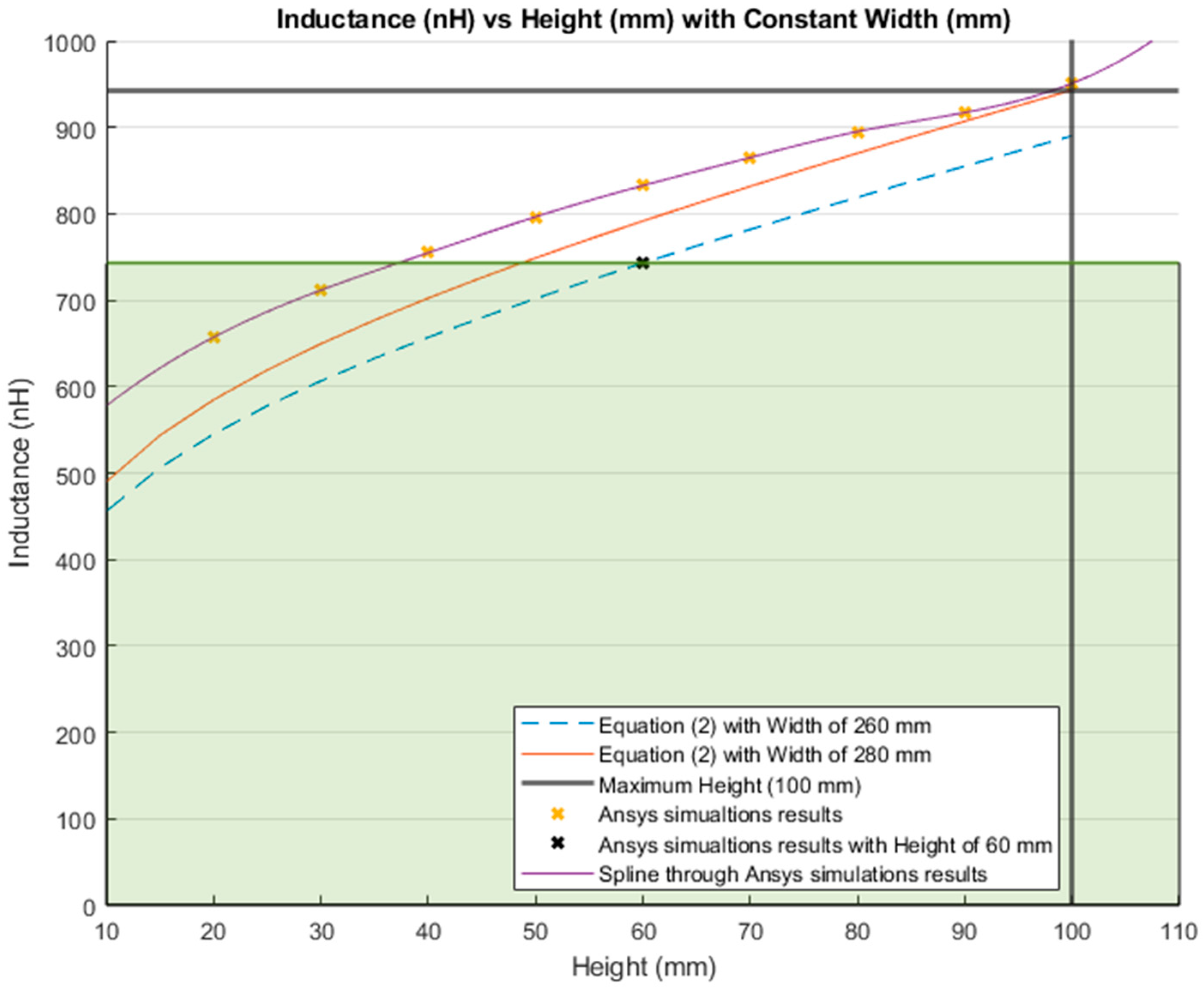
3.3.2. Comparison between Calculations and Simulations: Inductance Change Based on Height and Width
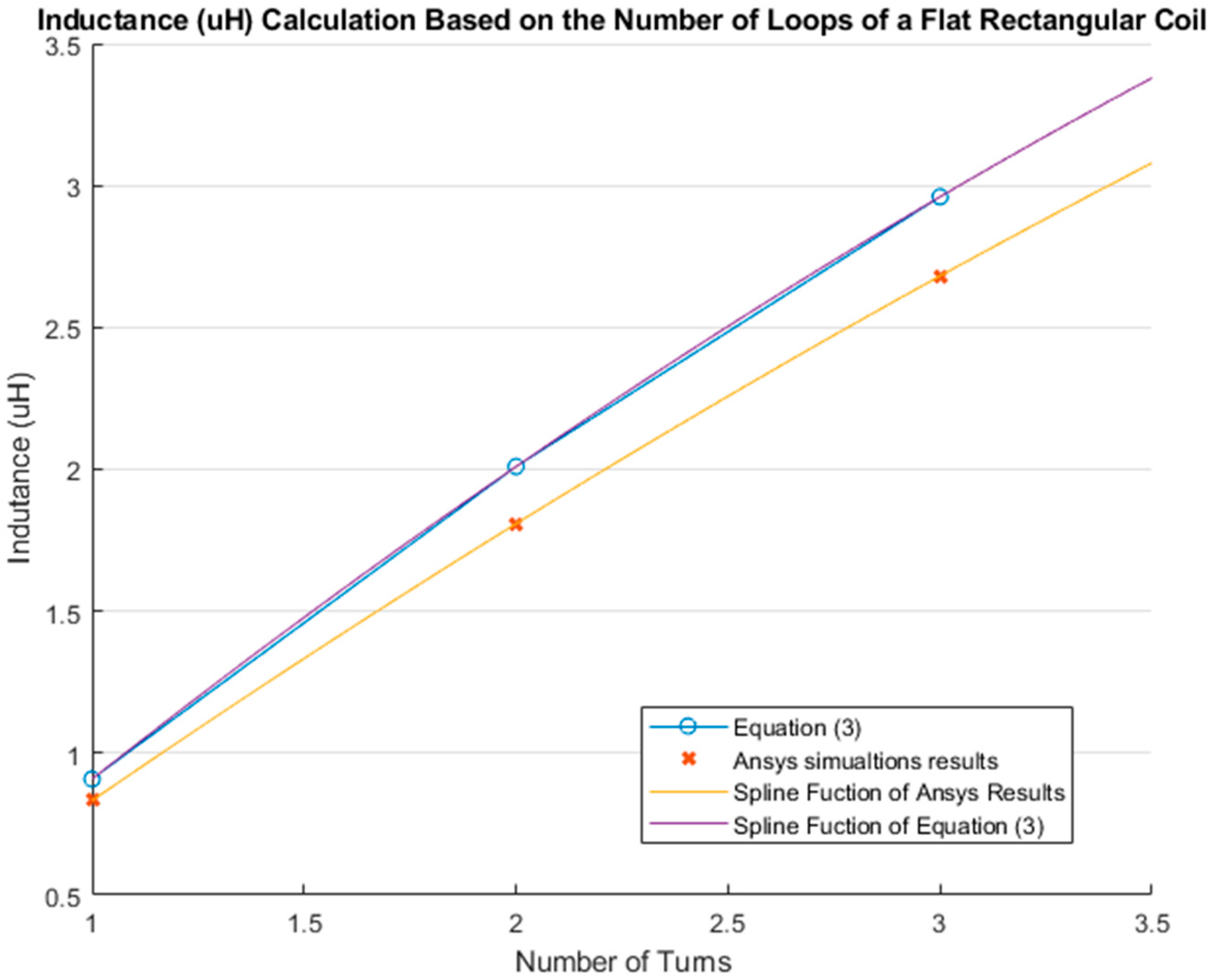
3.3.3. Comparison between Calculations and Simulations: Inductance Change Based on the Number of Loops in a Flat Rectangular Coil
4. Discussion
5. Conclusions
Author Contributions
Funding
Institutional Review Board Statement
Informed Consent Statement
Data Availability Statement
Conflicts of Interest
References
- Mokhlespour Esfahani, M.I.; Zobeiri, O.; Moshiri, B.; Narimani, R.; Mehravar, M.; Rashedi, E.; Parnianpour, M. Trunk motion system (TMS) using printed body worn sensor (BWS) via data fusion approach. Sensors 2017, 17, 112. [Google Scholar] [CrossRef] [PubMed]
- Atalay, O. Textile-Based, Interdigital, Capacitive, Soft-Strain Sensor for Wearable Applications. Materials 2018, 11, 765. [Google Scholar] [CrossRef] [PubMed]
- Patiño, A.G.; Khoshnam, M.; Menon, C. Wearable device to monitor back movements using an inductive textile sensor. Sensors 2020, 20, 5–8. [Google Scholar]
- Fava, J.O.; Lanzani, L.; Ruch, M.C. Multilayer planar rectangular coils for eddy current testing: Design considerations. NDT E Int. 2009, 42, 713–720. [Google Scholar] [CrossRef]
- Martinot-Lagarde, P.; Sartene, R.; Mathieu, M.; Durand, G. What does inductance plethysmography really measure? J. Appl. Physiol. 1988, 64, 1749–1756. [Google Scholar] [CrossRef] [PubMed]
- Catrysse, M.; Puers, R.; Hertleer, C.; van Langenhove, L.; van Egmond, H.; Matthys, D. Towards the integration of textile sensors in a wireless monitoring suit. Sens. Actuators A Phys. 2004, 114, 302–311. [Google Scholar] [CrossRef]
- Zhong, J.; Member, S.; Kiourti, A.; Sebastian, T. Conformal Load—Bearing Spiral Antenna on Conductive Textile Threads. IEEE Antennas Wirel. Propag. Lett. 2016, 16, 230–233. [Google Scholar] [CrossRef]
- Dionisi, A.; Marioli, D.; Sardini, E.; Serpelloni, M. Autonomous Wearable System for Vital Signs Measurement With Energy-Harvesting Module. IEEE Trans. Instrum. Meas. 2016, 65, 1423–1434. [Google Scholar] [CrossRef]
- Yoo, H.J. Your heart on your sleeve: Advances in textile-based electronics are weaving computers right into the clothes we wear. IEEE Solid-State Circuits Mag. 2013, 5, 59–70. [Google Scholar]
- Coosemans, J.; Hermans, B.; Puers, R. Integrating wireless ECG monitoring in textiles. Sens. Actuators A Phys. 2006, 130–131, 48–53. [Google Scholar] [CrossRef]
- Koo, H.R.; Lee, Y.J.; Gi, S.; Khang, S.; Lee, J.H.; Lee, J.H.; Lim, M.G.; Park, H.J.; Lee, J.W. The effect of textile-based inductive coil sensor positions for heart rate monitoring. J. Med. Syst. 2014, 38, 2. [Google Scholar] [CrossRef] [PubMed]
- Wijesiriwardana, R. Inductive fiber-meshed strain and displacement transducers for respiratory measuring systems and motion capturing systems. IEEE Sens. J. 2006, 6, 571–579. [Google Scholar] [CrossRef]
- Wu, D.; Wang, L.; Zhang, Y.T.; Huang, B.Y.; Wang, B.; Lin, S.J.; Xu, X.W. A wearable respiration monitoring system based on digital respiratory inductive plethysmography. In Proceedings of the 2009 Annual International Conference of the IEEE Engineering in Medicine and Biology Society, Minneapolis, MN, USA, 3–6 September 2009; pp. 4844–4847. [Google Scholar]
- Gonçalves, C.; da Silva, A.F.; Gomes, J.; Simoes, R. Wearable E-Textile Technologies: A Review on Sensors, Actuators and Control Elements. Inventions 2018, 3, 14. [Google Scholar] [CrossRef]
- Bonroy, B.; Meijer, K.; Dunias, P.; Cuppens, K.; Gransier, R.; Vanrumste, B. Ambulatory Monitoring of Physical Activity Based on Knee Flexion/Extension Measured by Inductive Sensor Technology. ISRN Biomed. Eng. 2013, 2013, 1–10. [Google Scholar] [CrossRef]
- Pheasant, S. Bodyspace Anthropometry, Ergonomics and the Design of Work, 2nd ed.; Taylor & Francis: London, UK, 2003; Volume 1. [Google Scholar]
- Thompson, M.T. Inductance Calculation Techniques—Part II: Approximations and Handbook Methods. Power Control Intell. Motion 1999, 11. [Google Scholar]
- Terman, F.E. Radio Engineers’ Handbook, 1st ed.; McGraq-Hill Book Company Inc.: New York, NY, USA, 1943. [Google Scholar]
- Grover, F.W. Methods, formulas, and tables for the calculation of antenna capacity. Sci. Pap. Bur. Stand. 1926, 22, 569. [Google Scholar] [CrossRef][Green Version]
- Sardini, E.; Serpelloni, M.; Ometto, M. Smart vest for posture monitoring in rehabilitation exercises. In Proceedings of the 2012 IEEE Sensors Applications Symposium Proceedings, Brescia, Italy, 7–9 February 2012; pp. 161–165. [Google Scholar]
- Tavassolian, M.; Cuthbert, T.J.; Napier, C.; Peng, J.; Menon, C. Textile-Based Inductive Soft Strain Sensors for Fast Frequency Movement and Their Application in Wearable Devices Measuring Multiaxial Hip Joint Angles during Running. Adv. Intell. Syst. 2020, 2, 1900165. [Google Scholar] [CrossRef]
- Atalay, O.; Tuncay, A.; Husain, M.D.; Kennon, W.R. Comparative study of the weft-knitted strain sensors. J. Ind. Text. 2017, 46, 1212–1240. [Google Scholar] [CrossRef]
- Atalay, O.; Kennon, W.R.; Dawood, M. Husain Textile-based weft knitted strain sensors: Effect of fabric parameters on sensor properties. Sensors 2013, 13, 11114–11127. [Google Scholar] [CrossRef]
- Vogl, A.; Parzer, P.; Babic, T.; Leong, J.; Olwal, A.; Haller, M. StretchEBand: Enabling Fabric-Based Interactions through Rapid Fabrication of Textile Stretch Sensors. In Proceedings of the CHI 2017 (SIGCHI Conference on Human Factors in Computing Systems), Denver, CO, USA, 6–11 May 2017; pp. 2617–2627. [Google Scholar]
- Paradiso, R.; Loriga, G.; Taccini, N. A wearable health care system based on knitted. IEEE Trans. Inf. Technol. Biomed. 2005, 9, 337–344. [Google Scholar] [CrossRef]
- Mattmann, C. Body Posture Detection Using Strain Sensitive Clothing; ETH: Zurich, Switzerland, 2008. [Google Scholar]
- Bjørk, I.T.; Samdal, G.B.; Hansen, B.S.; Tørstad, S.; Hamilton, G.A. Job satisfaction in a Norwegian population of nurses: A questionnaire survey. Int. J. Nurs. Stud. 2007, 44, 747–757. [Google Scholar] [CrossRef] [PubMed]
- Castel, E.S.; Ginsburg, L.R.; Zaheer, S.; Tamim, H. Understanding nurses’ and physicians’ fear of repercussions for reporting errors: Clinician characteristics, organization demographics, or leadership factors? BMC Health Serv. Res. 2015, 15, 1–10. [Google Scholar] [CrossRef] [PubMed]
- Ang, S.Y.; Dhaliwal, S.S.; Ayre, T.C.; Uthaman, T.; Fong, K.Y.; Tien, C.E.; Zhou, H.; Della, P. Demographics and Personality Factors Associated with Burnout among Nurses in a Singapore Tertiary Hospital. BioMed Res. Int. 2016, 2016. [Google Scholar] [CrossRef] [PubMed]
- Churchill, E.; Laubach, L.L.; Mcconville, J.T.; Tebbetts, I. Anthropometric Source Book. Volume 1: Anthropometry for Designers. Available online: https://msis.jsc.nasa.gov/sections/section03.htm#_3.3_ANTHROPOMETRIC_AND. (accessed on 18 June 2020).
- Wang, M.; Leger, A.B.; Dumas, G.A. Prediction of back strength using anthropometric and strength measurements in healthy females. Clin. Biomech. 2005, 20, 685–692. [Google Scholar] [CrossRef] [PubMed]
- Marras, W.S.; Jorgensen, M.J.; Granata, K.P.; Wiand, B. Female and male trunk geometry: Size and prediction of the spine loading trunk muscles derived from MRI. Clin. Biomech. 2001, 16, 38–46. [Google Scholar] [CrossRef]
- Podbevšek, T. For a good fitted skirt, the waist-to-hip distance should be measured. Anthropol. Notebooks 2014, 20, 77–88. [Google Scholar]
- FreeSVG.org. Human Male and Female Body Line Art. Available online: https://freesvg.org/1549491622 (accessed on 14 August 2020).
- Wikimedia Commons. Columna Vertebras.jpg. Available online: https://commons.wikimedia.org/wiki/File:Columna_vertebras.jpg (accessed on 14 August 2020).
- Wikimedia Commons. Human body silhouette.svg. Available online: https://commons.wikimedia.org/wiki/File:Human_body_silhouette.svg (accessed on 14 August 2020).


| Wire Diameter/D | A |
|---|---|
| 0.01 | −4.048 |
| 0.02 | −3.355 |
| 0.03 | −2.950 |
| 0.04 | −2.662 |
| 0.05 | −2.439 |
| 0.06 | −2.256 |
| 0.07 | −2.102 |
| 0.08 | −1.969 |
| 0.09 | −1.851 |
| 0.1 | −1.746 |
| Number of Turns (n) | B |
|---|---|
| 1 | 0.000 |
| 2 | 0.114 |
| 3 | 0.166 |
| 4 | 0.197 |
| 5 | 0.218 |
| 6 | 0.233 |
| 7 | 0.244 |
| 8 | 0.253 |
| 9 | 0.260 |
| 10 | 0.266 |
| Ansys’ Parameters | Sensor | |
|---|---|---|
| Sensor’s Characteristics | Between Connections | 10 mm |
| Total Height | 60 mm | |
| Total Length | 50 mm | |
| Material | Copper, Silver, Gold, Stainless steel | |
| Wire Diameter | 0.14 mm | |
| Box Characteristics | X | 150 mm |
| Y | 120 mm | |
| Z | 100 mm | |
| Material | Air | |
| Setup | Maximum # Passes | 10 |
| % Error | 1 | |
| % Refinement Per Pass | 30 | |
| Minimum # of Passes | 5 | |
| Minimum Converged Passes | 1 | |
| Trunk’s Anthropometry | |
|---|---|
| Trunk width at the iliac crest | 28 cm |
| Trunk length C7–L5 | 41.7 to 42.5 cm |
| Waist height | 103.4 cm |
| Trochanteric height | 82.4 cm |
| Ansys’ Parameters | Sensor | |
|---|---|---|
| Sensor’s Characteristics | Material | Copper |
| Wire Diameter | 0.14 mm | |
| Box Characteristics | X | 600 mm |
| Y | 150 mm | |
| Z | 100 mm | |
| Material | Air | |
| Setup | Maximum # Passes | 10 |
| % Error | 1 | |
| % Refinement Per Pass | 30 | |
| Minimum # of Passes | 5 | |
| Minimum Converged Passes | 1 | |
| Mesh | Classic, Small | -- |
| Excitation | -- | 1.56 mA |
| Perimeter (mm) | Width (mm) | Height (mm) |
|---|---|---|
| 556 | 200 | 78 |
| 581.82 | 220 | 70.91 |
| 610 | 240 | 65 |
| 640 | 260 | 60 |
| 671.42 | 280 | 55.71 |
| 704 | 300 | 52 |
| 737.5 | 320 | 48.75 |
| Area (mm2) | Width (mm) | Height (mm) |
|---|---|---|
| 3100 | 310 | 10 |
| 6000 | 300 | 20 |
| 11,200 | 280 | 40 |
| 15,600 | 260 | 60 |
| 19,200 | 240 | 80 |
| 22,000 | 220 | 100 |
| 24,000 | 200 | 120 |
| 25,200 | 180 | 140 |
| 25,600 | 160 | 160 |
| Constant Height (60 mm) | Constant Width (260 mm) |
|---|---|
| Width (mm) | Height (mm) |
| 230 | 30 |
| 240 | 40 |
| 250 | 50 |
| 260 | 60 |
| 270 | 70 |
| 280 | 80 |
| 290 | 90 |
| Perimeter (mm) | Width (mm) | Height (mm) | Simulation Inductance (nH) | Equation (1) Inductance (nH) |
|---|---|---|---|---|
| 556 | 200 | 78 | 731.865 | 694.28 |
| 581.82 | 220 | 70.91 | 762.972 | 721.24 |
| 610 | 240 | 65 | 790.339 | 750.40 |
| 640 | 260 | 60 | 832.576 | 781.16 |
| 671.42 | 280 | 55.71 | 870.783 | 813.08 |
| 704 | 300 | 52 | 901.676 | 845.86 |
| 734.5 | 320 | 48.75 | 941.019 | 876.27 |
| Area (mm2) | Width (mm) | Height (mm) | Simulation Inductance (nH) | Equation (1) Inductance (nH) |
|---|---|---|---|---|
| 3100 | 310 | 10 | 680.557 | 574.33 |
| 6000 | 300 | 20 | 757.299 | 658.86 |
| 11,200 | 280 | 40 | 804.619 | 738.75 |
| 15,600 | 260 | 60 | 832.576 | 781.16 |
| 19,200 | 240 | 80 | 835.797 | 807.74 |
| 22,000 | 220 | 100 | 847.971 | 825.16 |
| 24,000 | 200 | 120 | 840.832 | 836.30 |
| 25,200 | 180 | 140 | 842.452 | 842.55 |
| 25,600 | 160 | 160 | 854.903 | 844.56 |
| Width (mm) | Simulations Inductance (nH) | Equation (2) Inductance (nH) |
|---|---|---|
| 230 | 743.565 | 670.09 |
| 240 | 769.836 | 694.39 |
| 250 | 795.330 | 718.70 |
| 260 | 821.577 | 742.99 |
| 270 | 846.542 | 767.29 |
| 280 | 871.462 | 791.57 |
| 290 | 896.130 | 815.86 |
| Height (mm) | Simulations Inductance (nH) | Equation (2) Inductance (nH) |
|---|---|---|
| 30 | 711.167 | 606.58 |
| 40 | 752.310 | 657.07 |
| 50 | 788.522 | 701.79 |
| 60 | 821.577 | 742.99 |
| 70 | 849.815 | 781.86 |
| 80 | 874.200 | 819.08 |
| 90 | 893.009 | 855.08 |
Publisher’s Note: MDPI stays neutral with regard to jurisdictional claims in published maps and institutional affiliations. |
© 2021 by the authors. Licensee MDPI, Basel, Switzerland. This article is an open access article distributed under the terms and conditions of the Creative Commons Attribution (CC BY) license (http://creativecommons.org/licenses/by/4.0/).
Share and Cite
Patiño, A.G.; Menon, C. Inductive Textile Sensor Design and Validation for a Wearable Monitoring Device. Sensors 2021, 21, 225. https://doi.org/10.3390/s21010225
Patiño AG, Menon C. Inductive Textile Sensor Design and Validation for a Wearable Monitoring Device. Sensors. 2021; 21(1):225. https://doi.org/10.3390/s21010225
Chicago/Turabian StylePatiño, Astrid García, and Carlo Menon. 2021. "Inductive Textile Sensor Design and Validation for a Wearable Monitoring Device" Sensors 21, no. 1: 225. https://doi.org/10.3390/s21010225
APA StylePatiño, A. G., & Menon, C. (2021). Inductive Textile Sensor Design and Validation for a Wearable Monitoring Device. Sensors, 21(1), 225. https://doi.org/10.3390/s21010225