1. Introduction
Due to the pervasivenss of real-time and critical systems like Internet of Things (IoT) platforms, automotives, and robotics, new types of requirements are being addressed in the use of Deep Neural Networks (DNNs).
The main challenges when dealing with DNNs are both the ubiquitous multiply-and-accumulate operations and the massive use of activation functions across the neural network layers. A big speed-up to these challenges is surely offered by parallelization of the workloads (e.g., Graphics Processing Units (GPUs) or Single-Instruction Multiple-Data (SIMD)) processors). However, these solutions are considerable demanding in terms of resources. Moreover, adding parallelization in critical systems may reduce the predictability of the said system (see References [
1,
2]). Furthermore, even the use of floating point SIMD engines is not always possible in embedded systems (e.g., ARM Cortex-M4 [
3]). This means that we cannot always rely on high-performance processing units in critical and real time scenarios, thus needing to address new challenges.
Therefore, the challenging topic is to satisfy the real-time requirements while guaranteeing computational efficiency and lowering the power and the cost of such applications. One of the main paths to reduce the computational complexity when evaluating DNNs is stepping away from cumbersome arithmetic such as double-precision floats (represented on 64 bit). The basic idea is to use compressed formats that may save resources in terms of power consumption and computational efficiency. Great examples of compact formats are Brain Floats (BFLOAT) and Flexpoint [
4,
5] that consist in an optimized version of the 16-bit standard floating point number IEEE 754) used by Google for their TPU (tensor processing unit) engines. Other formats also come from the concept of transprecision computing [
6,
7] (NVIDIA Turing architectures allow computation with 4-, 8-, and 32-bit integers and with 16- and 32-bit floats). The up-and-coming Posit format has been theoretically [
8,
9,
10] and practically [
11] proven to be a perfect replacement for IEEE float numbers when applied to DNNs in terms of efficiency and accuracy.
Due to its novelty, this format lacks proper or standardized hardware support (e.g., a Posit Processing Unit (PPU)) to accelerate its computation, forcing the use of software implementations. However, in order to speed up the software emulation of Posits in DNNs, we present two different techniques. In this paper, we extend the work on deriving a fast and approximate version of the hyperbolic tangent (TANH) presented in Reference [
12]. We introduce novel arithmetic properties of the Posit number system with a deep focus on the Posits with 0 exponent bits. This special case allows us to build common functions and arithmetic operators as simple bit manipulations on the bit-string representing a Posit number. This new class of functions (called L1 functions) has some interesting properties:
The operation evaluation is faster than its counterpart with little to no degradation on accuracy.
Since these operations only need integer arithmetic and logic operations, they are straightforwardly executed in the already existing ALU, also allowing a faster emulation of Posits
Being able to write functions as a sequence of arithmetic-logic operations allows us to vectorize them exploiting already existing SIMD (Single Instruction–Multiple Data) engines.
In particular, in this extension, we also propose a new fast and approximated version of the Extended Linear Unit (ELU) activation function.
Moreover, if we consider really low-power devices that do not embed a floating point unit but only an arithmetic logic unit, the approach proposed can become very interesting to enable DNN processing even in this class of devices (although for inference only, not for training).
Furthermore, we investigate operator tabulation as a different approach to speed up Posit emulation without constraints on the exponent configuration. This allows us to accelerate basic arithmetic operators like sum and multiplication that are not suitable for being implemented as L1 functions. Although very powerful, this approach has clear limitations to its scalability, having a considerable spatial complexity.
Paper Structure
The paper is organized as follow:
Section 2 introduces the Posit format, proposing novel approaches to approximation and speed-up of Posit arithmetic, exploiting the 0-bit exponent Posit configuration.
Section 3 describes the cppPosit library implemented in Pisa for the computation of the new numerical format.
Section 4 introduces the hyperbolic tangent and ELU activation functions along with their approximations.
Section 5 shows the results of our approach with DNN and common benchmarking datasets. Finally,
Section 6 provides the conclusions.
2. Posit Arithmetic
The Posit format has been introduced by John L. Gustafson in Reference [
8] and was further investigated in Reference [
9,
10,
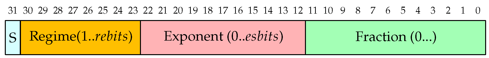
12]. The format is a fixed-length one with up to 4 fields as also reported in
Figure 1:
Sign field: 1-bit
Regime field: variable length, composed of a string of bits equal to 1 or 0 ended respectively by a 0 or 1 bit.
Exponent field: at most es bits
Fraction field: variable length mantissa
Given a Posit on
, represented by the integer
X, and
e and
f respectively as the exponent and fraction values, the real number
r represented by that encoding is as follows:
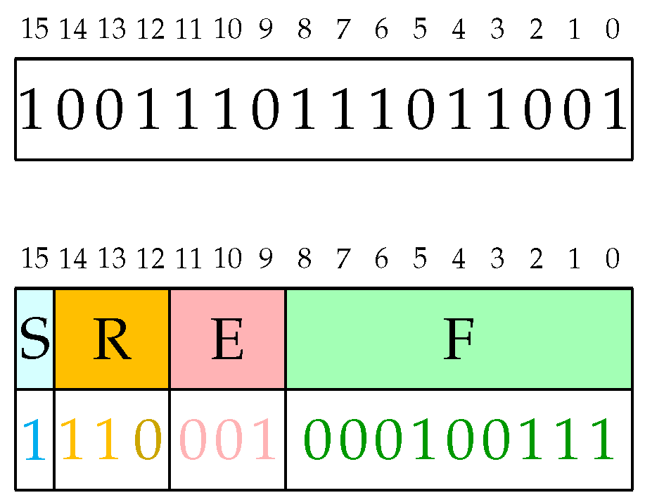
An example of Posit decoding operation is shown in
Figure 2.
The design of a hardware Posit Processing Unit (PPU) as a replacement for the FPU has already started on several universities worldwide, but it will take time for their availability on real platforms. Fortunately, we can still do many things related to DNNs even in the absence of a hardware PPU. Furthermore, when DNN weights can be represented with less than 14-bit Posits, we can tabulate some core operations like sum and multiplication (see
Section 3.1) and can use the ALU for other operations that will be shown hereafter in order to reduce the number of tables.
As reported above, the process of decoding a Posit involves the following steps: obtaining regime value by reconstructing the bit-string, building exponent, and extracting fraction. We can make use of C low-level building blocks to speed up the decoding:
Count leading zeros: using the embedded
__builtin_clz C function that several CPU families provide in hardware [
13].
Next power of two: used to extract the fraction. An efficient way to obtain the next power of two, given a representation X on 32 bit, is the following:
next_p2(X) -> Y
Y = X - 1
Y = Y | X >> 1
Y = Y | X >> 2
Y = Y | X >> 4
Y = y | X >> 8
Y = Y | X >> 16
Y = Y + 1
This approach copies the highest set bit to all the lower bits. Adding one to such a string will result in a sequence of carries that will set all the bits from the highest set to the least significant one to 0 and the next (in order of significancy) bit of the highest set to 1, thus producing the next power of two. Let us use an example. Suppose . At the first step, . At the second step, . At the next step, . From now on, Y will remain set to . At the last step, , that is the next power of two starting from 5.
2.1. The Case of No Exponent Bits (esbits = 0)
When using a Posit configuration with zero exponent bits (
esbits = 0), some interesting properties arise. In this case, we can express the real number represented by the Posit as follows:
where
is the fraction field and
F the fraction length. The value of
k depends on the regime length R. In particular,
for
(from now on
) and
for
(from now on
). If we denote the bit immediately following the regime bit string (stop-bit) as
, we can express the value of
R as
, where
is the position of the stop-bit in the Posit bit-string. For
, we can note that, substituting the expression for
in (
1), we get the following expression:
Moreover, we can link
with its representation
X using Equation (
3), obtaining:
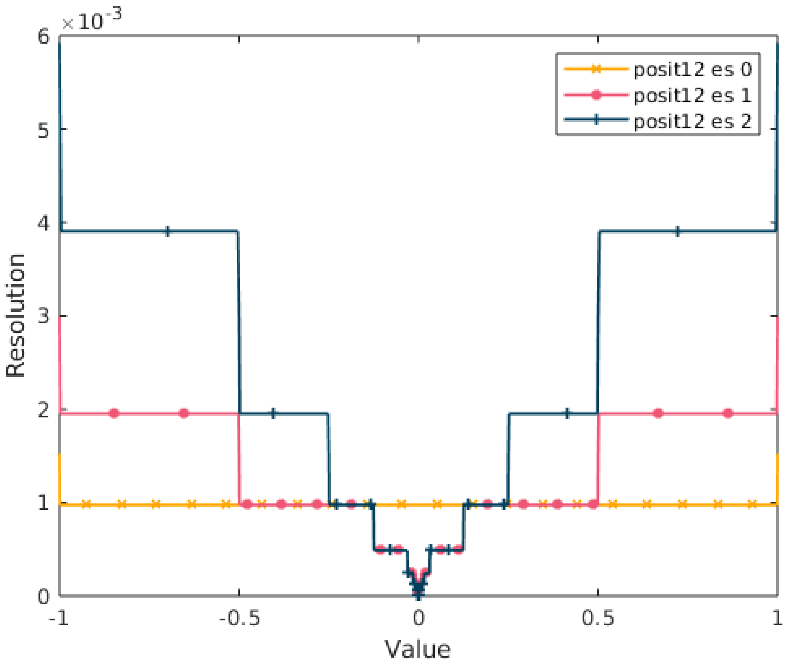
A particular property emerges with 0-bit exponent Posits when considering the
range. In fact, if we plot the resolution (that is the decimal difference between the real numbers represented by two consecutive bit-strings) of a Posit
in
we obtain the resolution of a fixed-point format. This property is visualized in
Figure 3. This is a very important property that will be exploited below.
As we will see below, the novel equations introduced above for the first time play an important role for deriving fast approximation of activation functions in DNNs. Equation (
3) says also that a Posit with zero exponent bits can be interpreted as a fixed point number with a shift of
bits. This has implications on the accuracy and further operations.
An example of how to exploit the expressions discovered in the previous section is building a fast approximated inversion operator. Given
x, we want to find a fast and efficient way to compute
y such that
. In the following, we will consider only positive values of x. The simplest case is when
. Let us consider
; we simply need to apply a reduction of the regime length by 1 as in Equation (
4).
A trickier case is when
. Here, we can easily see that
, that implies
. Therefore, we get Equation (
5).
Then, discarding the term
, we obtain Equation (
6):
The latter can be obtained by simply bitwising-not
and by adding 1, thus obtaining Equation (
7):
where ⊕ is the exclusive or (XOR) operator, ¬ is the bitwise negation operator, and
signmask is the a mask obtained as shown in the following pseudo-code. For example, given a 5-bit Posit, the signmask is simply
. The pseudocode also takes into account the holder size; in fact, a 5-bit Posit may be held by an 8-bit integer. This means that, for this holder type, the signmask produced by the pseudocode is
.
A pseudo-code implementation for (otherwise, we simply invert the sign) is as follows:
inv(x) -> y
X = x.v // ’v’ field: bit-string representing the Posit
msb = 1 << (N-1)
signmask = ~((msb | msb -1) >> 1)
Y = X ^ (~signmask) // negation operator followed by XOR operator (C-style)
y(Y)
Another useful function to implement as bit manipulation is the one’s complement operator (
8)
This is of interest when
. In this case,
, of course. From Equations (
1) and (
2), we can rewrite the operator as in Equation (
9).
Since we can link
x to its representation
X, we obtain (
10).
Then, we can also link
y to
Y, obtaining (
11).
The latter can be obtained easily with an integer subtraction only using the ALU. A pseudo-code implementation is the following:
comp_one(x) -> y
X = x.v // ’v’ field: bit-string representing the Posit
invert_bit = 1 << (N-2)
Y = invert_bit - X
y(Y)
when , we know that . when doubling/halving x, we simply increment/decrement the exponent k by 1. For 0-bit exponent Posits, this operation corresponds to one left shift for doubling and one right shift for halving the number. For instance, let us take a Posit with the value . The correspondent bit-string will be . If we shift it by one position right, we will get , that is the bit-string corresponding to a Posit with value .
2.2. FastSigmoid
As pointed out in Reference [
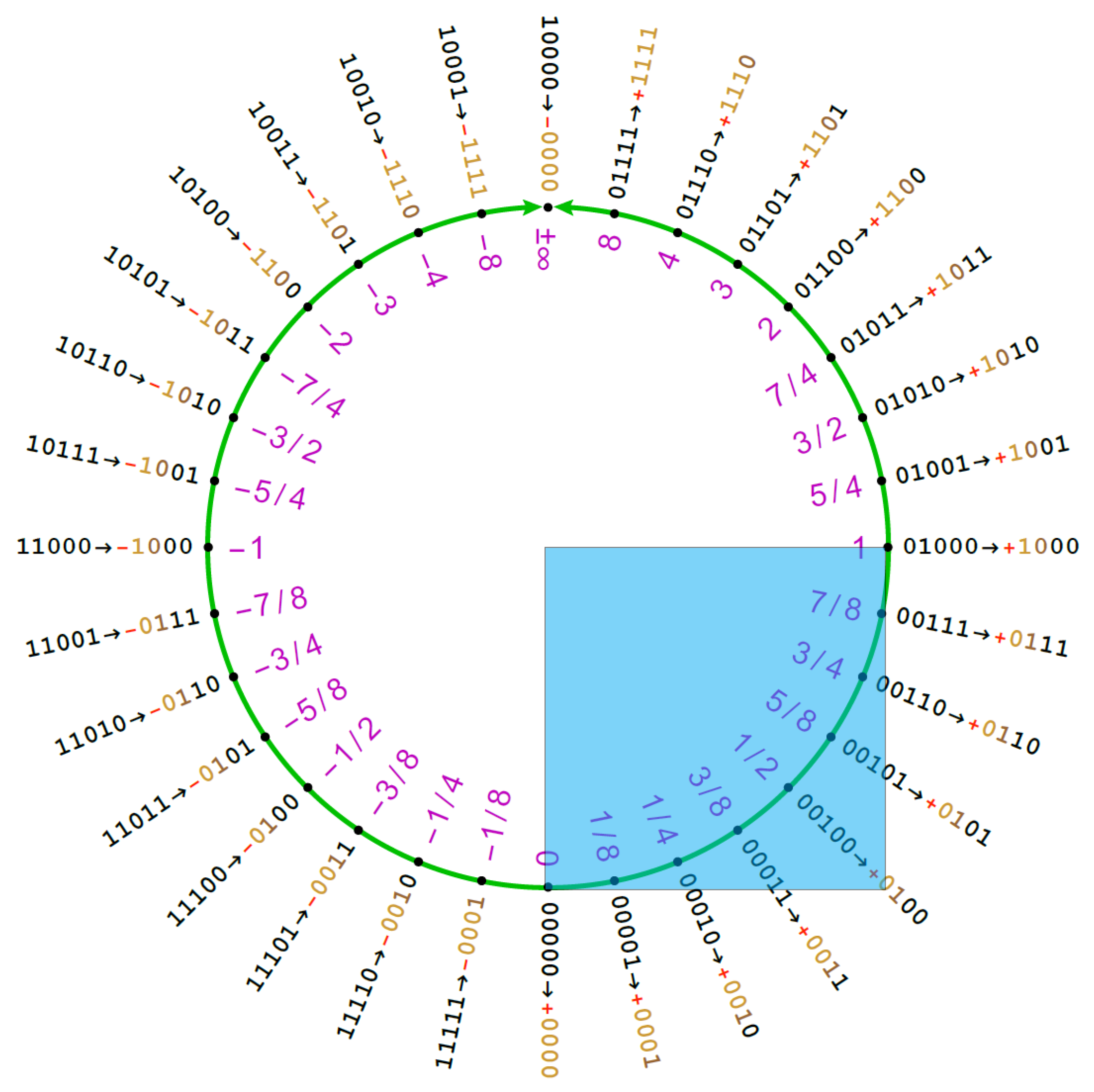
8], if we plot the 2’s complement value of the signed integer representing the Posit against the real number obtained from Equation (2), we obtain an S-shaped function very similar to the sigmoid curve. What we need to do is to rescale it to have the co-domain
and to shift it in order to center it in 0. To bring the Posit in
, we must notice that the quadrant is characterized by having the two most significant bits set at
00 (see
Figure 4).
Moreover, we can notice that adding the invert bit seen in previous sections to the Posit representation means moving it a quarter of the quadrant. In fact with , when adding the invert bit, we are adding , that is equal to , which is the number of Posits that fit in a single quarter of a ring. This means moving L times along the Posit ring, thus skipping a quarter of it. A pseudo-code implementation of this transformation is the following:
fastSigmoid(x) -> y
X = x.v // ’v’ field: bit-string representing the Posit
Y = (invert_bit + (X >> 1)) >> 1
y(Y)
In order to understand how this code works, we need to separate the analysis for
and
, considering only positive values, since the reasoning is symmetric for negative ones.
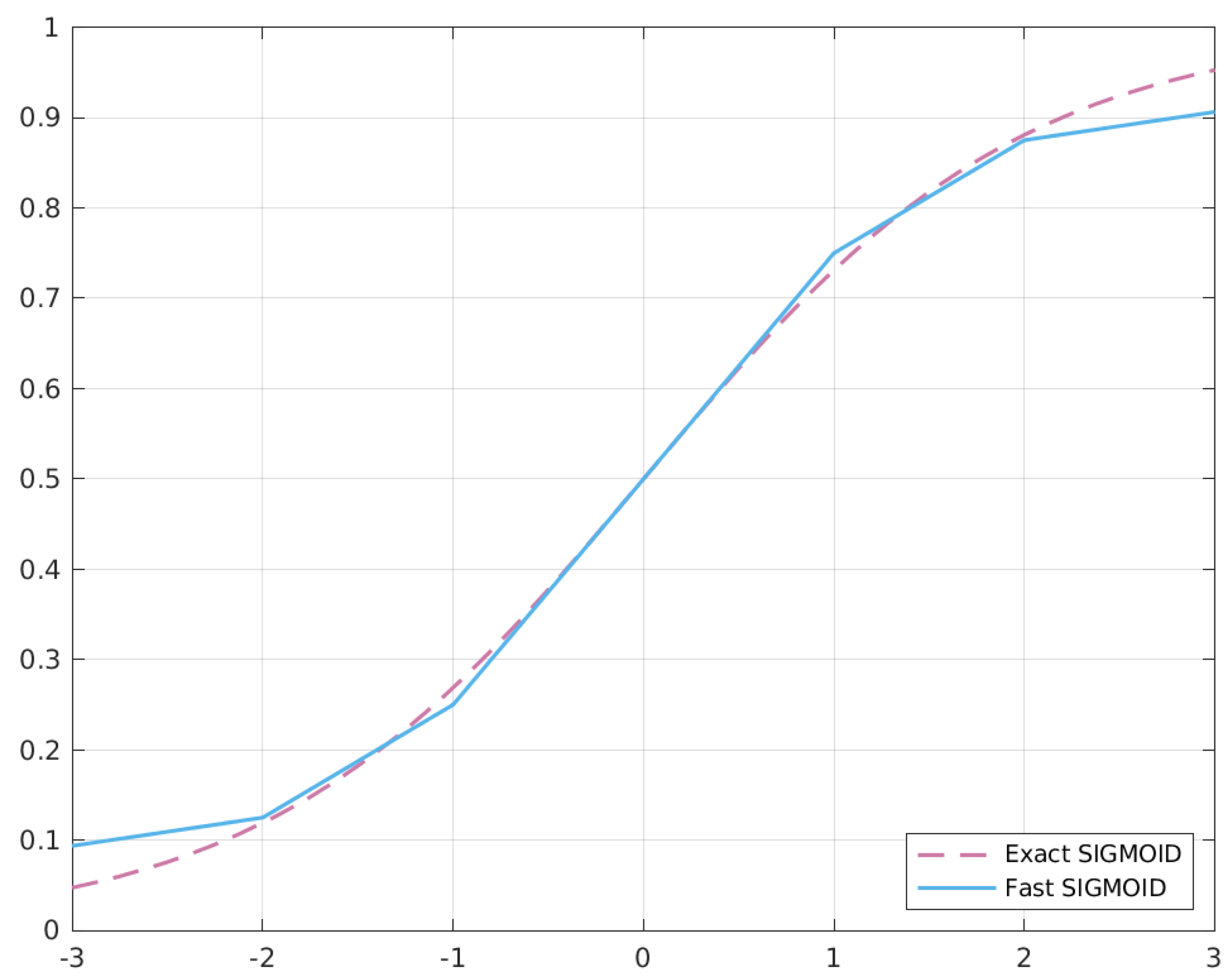
Figure 5 shows the behaviour of the two sigmoid versions.
We know that, for values of
, the behaviour of
x is like the one of a fixed point representation, so the first right shift is simply a division by two. When we add the
invert bit, we move the Posit in the northeast ring quarter (
). After this addition, the last shift can be considered as a division by two as well, thus obtaining the following:
Equation (
12) is also the first-order Taylor expansion of the Sigmoid function in
.
With
x represented as the bit-string
, the right shift will produce
. Now, with some computation, we can express
as a function of
x and
, obtaining (
13).
when adding the
invert bit, we obtain
. Finally, with the last right shift, we obtain (
14).
We know that we can approximate
. If we substitute it back in Equation (
14), we obtain Equation (
15), close to
:
3. CppPosit Library
For this paper, we employ our software implementation of Posit numbers developed at the University of Pisa, called cppPosit. As already described in References [
9,
12], the library classifies Posit operations into four different classes (from L1 to L4), with increasing computational complexity.
Among the others, L1 operations are the ones we want to focus on, since they can be fully emulated with an ALU. For this reason, they provide means to produce very efficient operators, as reported in
Table 1.
This level supports Posit reciprocation and sign-negation as well as one’s complement. Furthermore, when dealing with 0 exponent-bit configuration, they provide the fast and approximated sigmoid function (FastSigmoid) as described in Reference [
8] and the fast approximation of the hyperbolic tangent (FastTanh) investigated in Reference [
12]. Other interesting operators that require 0 exponent bits are the double and half functions. It is clear that, given these requirements, it is not always easy to derive a simple expression for a particular function that can be implemented in an L1 way. However, the effort put in this step is completely rewarded since it brings both faster execution both in a emulated and hardware Posit Processing Unit (PPU) and reduction of transistor occupation when dealing with hardware implementation of the unit.
3.1. Tabulated Posits
In the absence of proper hardware support of a Posit Processing Unit (PPU), there still is the need for speeding up the computation. An interesting mean to cope with this problem is the pre-computation of some useful Posit operators in look-up tables. These lookup tables (LUTs) become useful when the number of bits is low (e.g., ). The core idea is to generate tables for the most important arithmetic operations (addition/subtraction and multiplication/division) for all combinations of a given Posit configuration . Moreover, some interesting functions can be tabulated in order to speed up their computation, like logarithm or exponentiation. Given an bit Posit with a naive approach, a table will be where .
Depending on the underlying storage type T, each table entry will occupy b=sizeof(T) bits. Typically, there will be between and tables for a Posit configuration. This means that the overall space occupation will be .
Table 2 shows different per-table occupations of different Posit configurations. As reported, only Posits with 8 and 10 bits have reasonable occupation, considering current generation of CPUs. In fact, we can obtain a considerable speed-up when one or more tables can be entirely contained inside the cache.
In order to reduce both LUT size and their number, we can exploit some arithmetic properties:
3.2. Type Proxying
When dealing with Posit configuration with it is not possible to exploit fast approximation of operators that relies on this property. A possible solution is to switch to a different Posit configuration with 0 exponent bits and higher total number of bits to exploit a fast approximation and to then switch back to the original one.
Increasing the number of bits is also useful when the starting Posit configuration has already 0 exponent bits. In fact, increasing for the operator computation increases the accuracy of the computation, avoiding type overflows.
Given a Posit configuration , the basic idea is to proxy through a configuration with . The core step in the approach is the Posit conversion between different configurations. The base case is converting , with and sizeof(T2)≫sizeof(T1). In this case, the conversion operation is the following:
convert0(p1) -> p2
v1 = p1.v // ’v’ field: bit-string representing the Posit
v2 = cast<T2>(v1) << (Z - X)
p2.v2 = v2
3.3. Brain Posits
The idea behind Brain Floats is to define a Float16 with the same number of bits for the exponents of an IEEE 754 Float32. BFloat16 is thus different from IEEE 754 Float16, and the rationale of its introduction is that, when we have a DNN already trained with IEEE Float32, we can perform the inference with a BFloat16 and we can expect a reduced impact on the accuracy due to the fact that the dynamic range of a BFloat16 is the same as that of IEEE Float32. Following the very same approach, we can define
Brain Posits to be associated to the Posit16 and Posit32 that will be standardized soon. In particular, BPosit16 can be designed in such a way that it has the same dynamic range of a standard Posit32, which will be the one with 2 bits of exponent. Since we are using the Posit format, we can define the BPosit16 as the 16-bit Posit having a number of bits for the exponent such that its dynamic range is similar to the one of Posit<32,2>. Using the same approach, we will define BPosit8, where the number of bits for the exponent, in this case, must be the one that allows the BPosit8 to cover most of the dynamic range of the standard 16-bit Posit, which is the Posit<16,1>. In the following, we will perform some computations to derive the two number of exponents. Indeed, another interesting aspect of type proxying is that we can also reduce the total number of bits while increasing the exponent ones and still being able to accommodate the entire dynamic range. In doing so, we need to know the minimum number of exponent bits of the destination type. Suppose we are converting from Posit
to Posit
, with
. We know that the maximum value for
(similarly, it holds for
as well) is
If we set the inequality
and we apply logarithms to both sides, we get
From this, we obtain the rule for determining the exponent bits of the destination type:
From Equation (
16), we can derive some interesting cases. A Posit
can be transformed into a Posit
without a significant loss in the dynamic range. Furthermore, the same holds for a Posit
, which can be approximated using Posit
.
For all this reasons, the Brain Posits proposed in
Table 5 might deserve a hardware implementation too.
4. Hyperbolic Tangent, Extended Linear Unit, and their Approximations
The hyperbolic tangent (
tanh from now on) is a commonly used activation function. Its use over the sigmoid function is interesting since it extends the sigmoid codomain to the interval
. This allows both the dynamic range of the sigmoid in the output to be exploited twice and the negative values in classification layers during training to be given meaning. The first advantage is particularly important when applied to Posit, especially to small-sized ones. In fact, when considering the sigmoid function, if we apply it to a Posit
, we practically obtain in the output the dynamic range of a Posit
, that is, for instance, quite limiting for Posits with 8 to 14 number of bits.
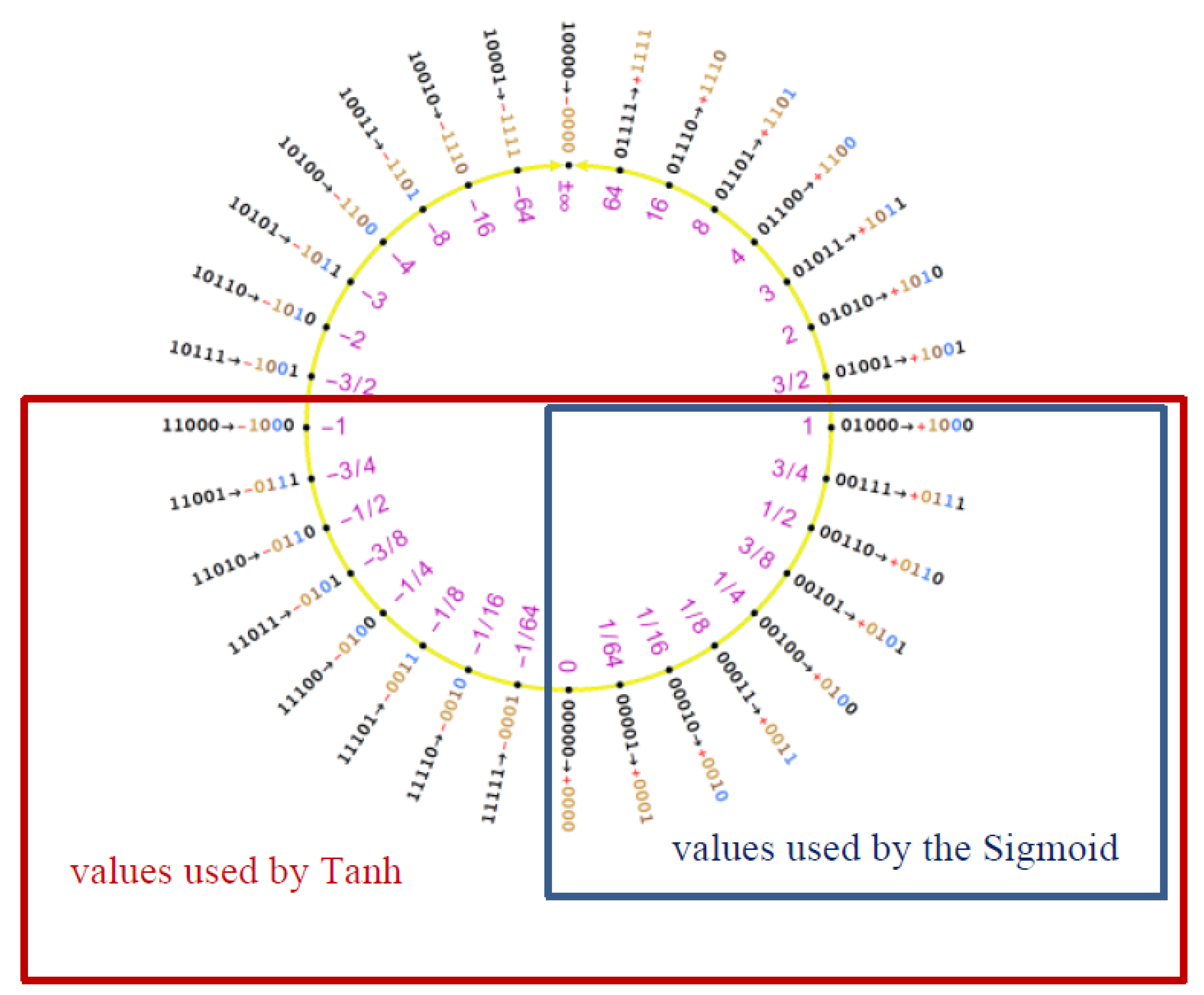
Figure 6 stresses this point, highlighting how the tanh function insists on the two most dense quarters of the Posit circle (the interval
occupies half of the Posit circle).
However, the sigmoid function has an important property, as shown in
Table 1 and in Reference [
8]: it can be implemented as L1 function, thus having a fast and efficient approximation only using integer arithmetics. The idea is to use the sigmoid function as a building block for other activation functions, only using a combination of L1 operators. We know that the sigmoid function is:
Now, we can scale and translate (
17) to cover the desired range
on the output obtaining the scaled sigmoid:
Equation (
18) is useful when setting
, thus obtaining the tanh expression in (
19):
From this formulation, we want to build an equivalent one that only uses L1 operators to build the approximated hyperbolic tangent, switching from sigmoid to the fast approximated version called FastSigmoid. Since we are dealing with 0 exponent bit Posits, the operations of doubling the Posit argument, computing the FastSigmoid, and doubling again is just a matter of bit manipulations, thus efficiently computed. However, the last step of subtracting 1 to the previous result is not an L1 operator out-of-the-box; thus, we reformulate the initial expression obtaining (
20):
If we consider only negative arguments
x, we know that the result of the expression
is always in the unitary region. This, combining with the 0 exponent bit hypothesis allows us to implement the inner expression with the 1’s complement L1 operator seen in
Table 1. The last negation is obviously an L1 operator; thus, we have the L1 fast approximation of the hyperbolic tangent in (
21):
Finally thanks to the antisymmetry of the tanh function, we can extend what we have done before to positive values. The following is a pseudo-code implementation:
FastTanh(x) -> y
x_n = x > 0 ? -x:x
s = x > 0
y_n = neg(compl1(twice(FastSigmoid(twice(x_n)))))
y = s > 0 ? -y_n:y_n
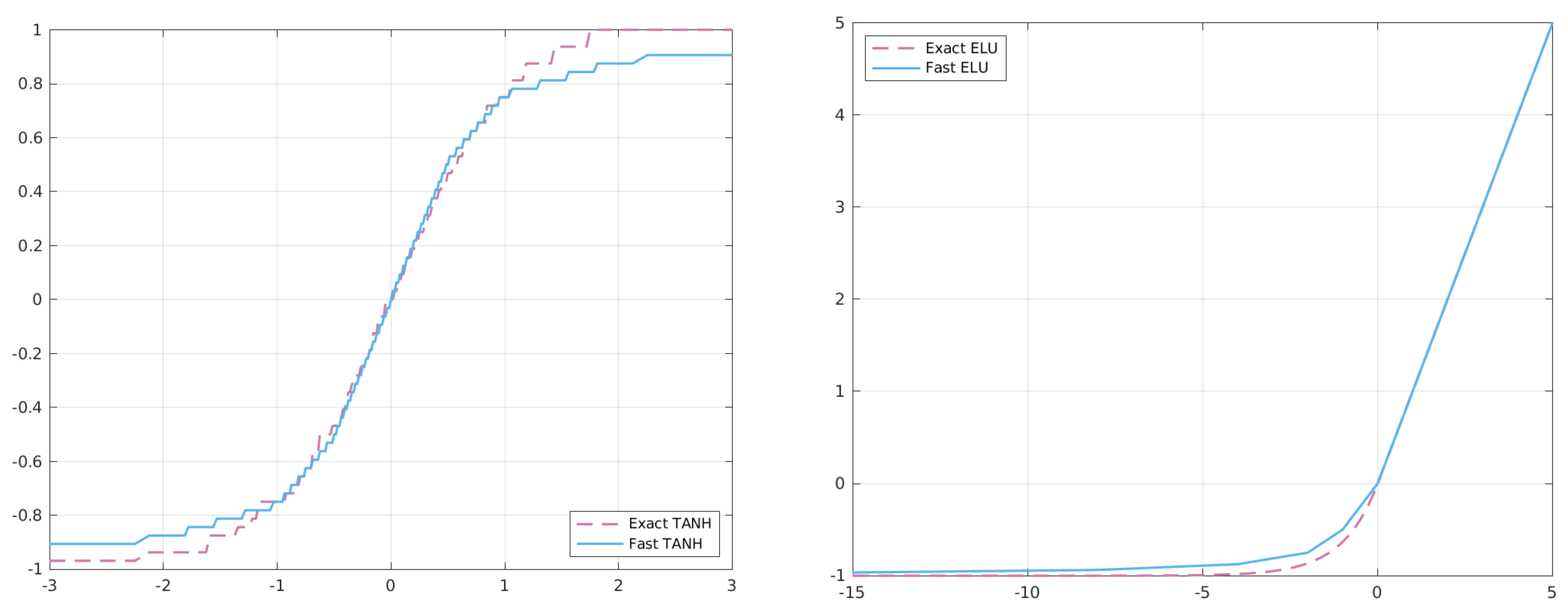
As already described, tanh and sigmoid functions can be implemented in their fast approximated version. However, the use of such kinds of shapes presents the well-known behaviour of vanishing gradients [
15]; for this reason, ReLU -like functions (e.g., ELU, Leaky-ReLU, and others) are preferable when dealing with a large number of layers in neural networks. As in Reference [
15], the ReLU activation function is defined as in (
22):
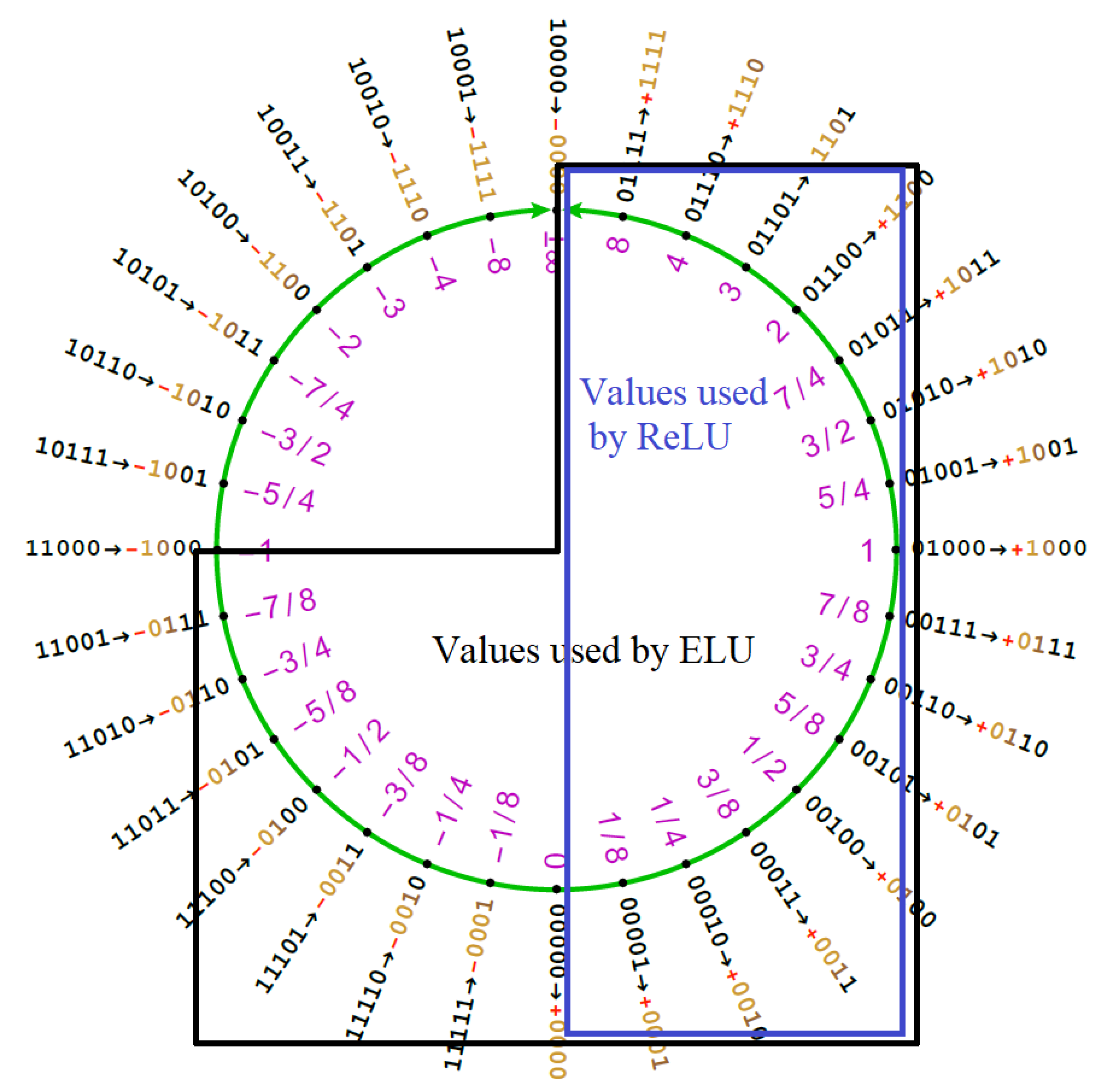
Its use is important in solving the vanishing gradient problem, having a non-flat shape towards positive infinity. However, when used with Posit numbers, this function can only cover , ignoring the very dense region .
In order to provide a more covering function with similar properties, we switch to the Extended Linear Unit (ELU) (
23):
This function is particularly interesting when
(
24), covering the missing dense region from the ReLU one:
Figure 7 shows the difference in Posit ring region usage of ELU and ReLU functions. It is remarkable how the ELU function manages to cover all the high density regions of the Posit ring. Moreover, the ELU function brings interesting normalization properties across the neural network layers as proven in Reference [
16]. This helps in keeping stable the range of variation of the weights of the DNN.
From Equation (
24), we can build a L1 approximation exploiting operators in
Table 1. The
behaviour for
is the identity function, that is L1 for sure. The first step for negative
x values is seeing that the ELU expression is similar to the reciprocate of Sigmoid function (
17). We can manipulate (
17) as follows:
We need to prove that the steps involved are L1 operations. The step in Equation (
25) is always L1 for
thanks to fast Sigmoid approximation. The result of this step is always on
. The step in Equation (26) is always L1, and the output is on
. The step in Equation (27) is always L1 for
, and the output is on
. The step in Equation (28) is L1 since the previous step output is in the unitary range
. The output of this step is in
as well. Finally, the last step is L1 for
. Expression (29) is exactly the ELU expression for negative values of the argument.
A pseudo-code implementation of the FastELU using only L1 operations is shown below:
FastELU(x) -> y
y_n = neg(twice(compl1(half(reciprocate(FastSigmoid(neg(x)))))))
y = x > 0 ? x:y_n
Figure 8 shows the behaviour of the two functions when approximated with our approach.
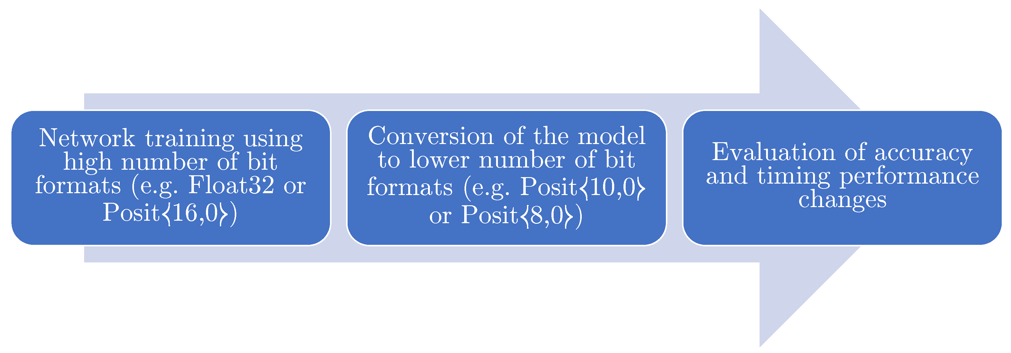
5. Implementation Results
In this section, the different proposed activation function performances are analyzed in both the exact and approximated fashions when used as activation function in the LeNet-5 neural network model [
17]. As shown in
Figure 9, the neural network is trained with the MNIST digit recognition benchmark (GTRSB) [
17] and the German Traffic Road Sign Benchmark [
18] datasets using the Float32 type. The performance metrics involved are the testing accuracy on said datasets and the mean sample inference time. Testing phase is executed converting the model to
type and to SoftFloat32 (a software implementation of floats). We used SoftFloats in order to ensure a fair comparison between the two software implementations due to the absence of proper hardware support for Posit type.
Benchmarks are executed on a 7th generation
Intel i7-7560U processor, running Ubuntu Linux
18.04, equipped with
GCC 8.3. Benchmark data is publicly available in References [
17]. The C++ source code can be downloaded from Reference [
19].
As reported in
Table 6 and
Table 7, the approximated hyperbolic tangent can replace the exact one, with a small degradation in accuracy but improving the inference time of about 2 ms in each Posit configuration. Moreover, the performance of FastTanh also overcome FastSigmoid in terms of accuracy. Furthermore, as reported in
Table 8 and
Table 9, the approximated ELU function can replace the exact one, with little-to-no accuracy degradation, improving the inference time of about 1 ms in each Posit configuration. Moreover, performance of FastELU also overcomes the ReLU in terms of accuracy, showing the benefits of covering the additional region in
. At the same time, the FastELU is not much slower than ReLU, thus being an interesting replacement to increase accuracy of Posits with few bits (e.g., Posit
) without losing too much in time complexity.
If we compare FastELU and FastTanh, their performance are quite similar in the benchmarks provided. However as already said in
Section 4, increasing the number of layers in the neural network model can lead to the so called “vanishing gradient” problem; s-shaped functions like sigmoid and hyperbolic tangent are prone to this phenomenon. This has been proven not to hold for ReLU-like functions.
The results highlight how Posits from to are a perfect replacement for float numbers; is a particularly interesting format since it offers the best data compression without any drop in accuracy. This reasonably makes the configuration of choice for low-precision inference when using Posits.


 . The final value is therefore (exact value, i.e., no rounding, for this case).


