UAV Autonomous Localization Using Macro-Features Matching with a CAD Model

 ,
, 
 and
and
Abstract
:1. Introduction
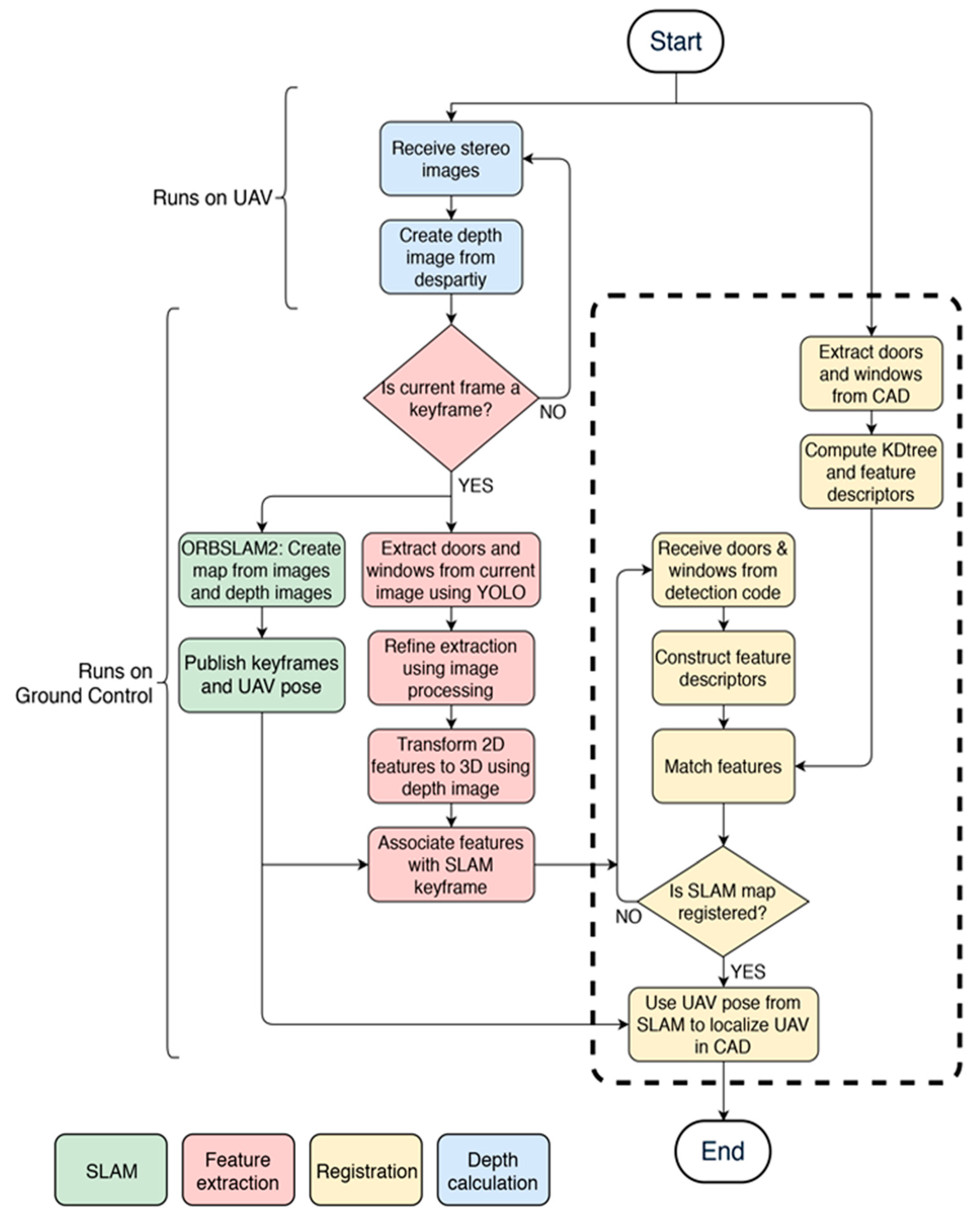
2. Methodology
2.1. Pre-Processing
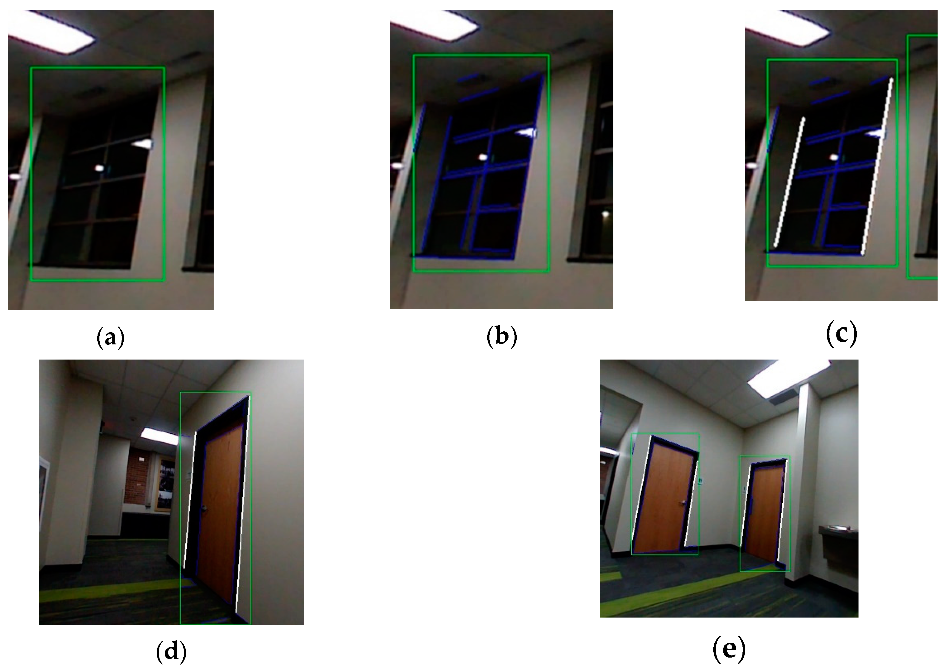
2.2. Macro-Feature Detection and Extraction Method
2.2.1. Data Preparation and Training
2.2.2. Detection Refinement
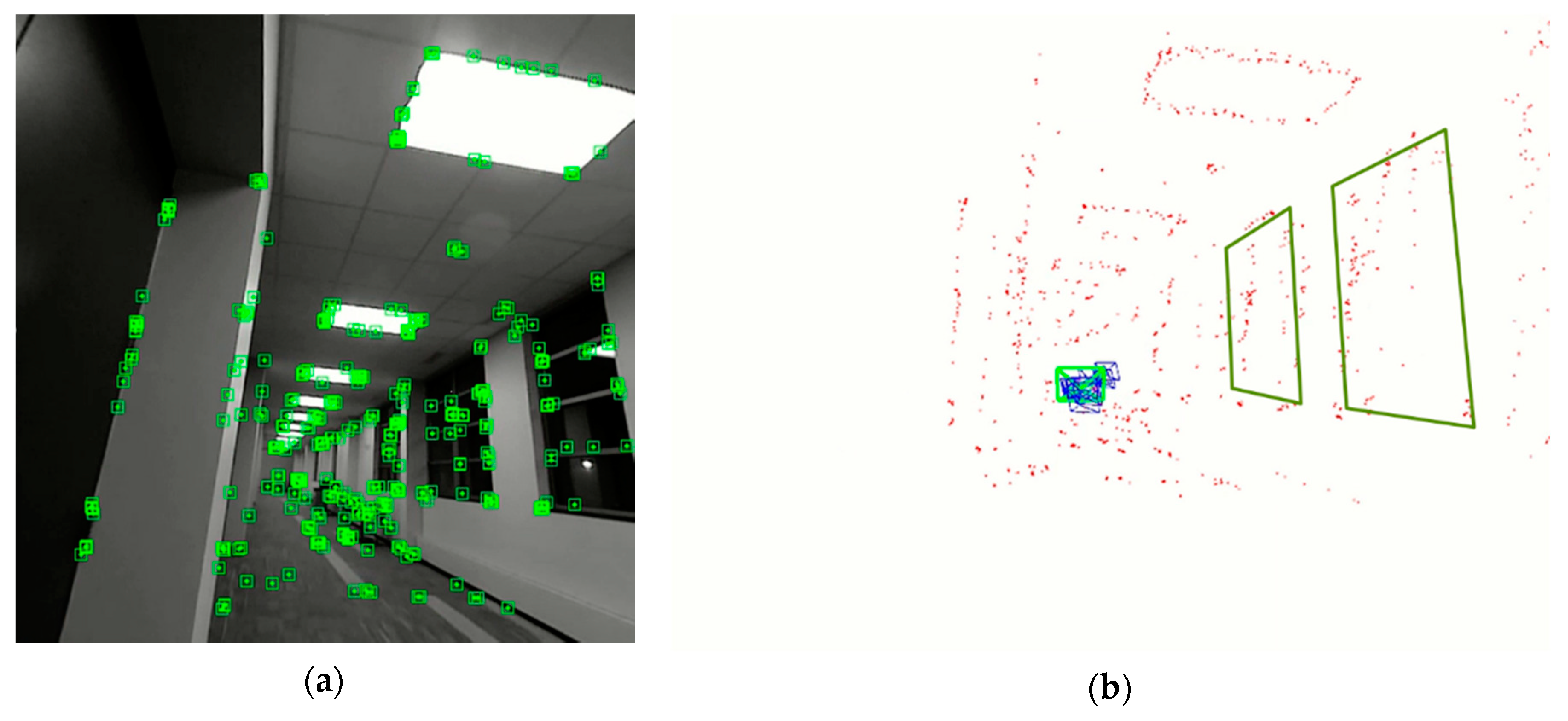
2.2.3. 3D Reconstruction
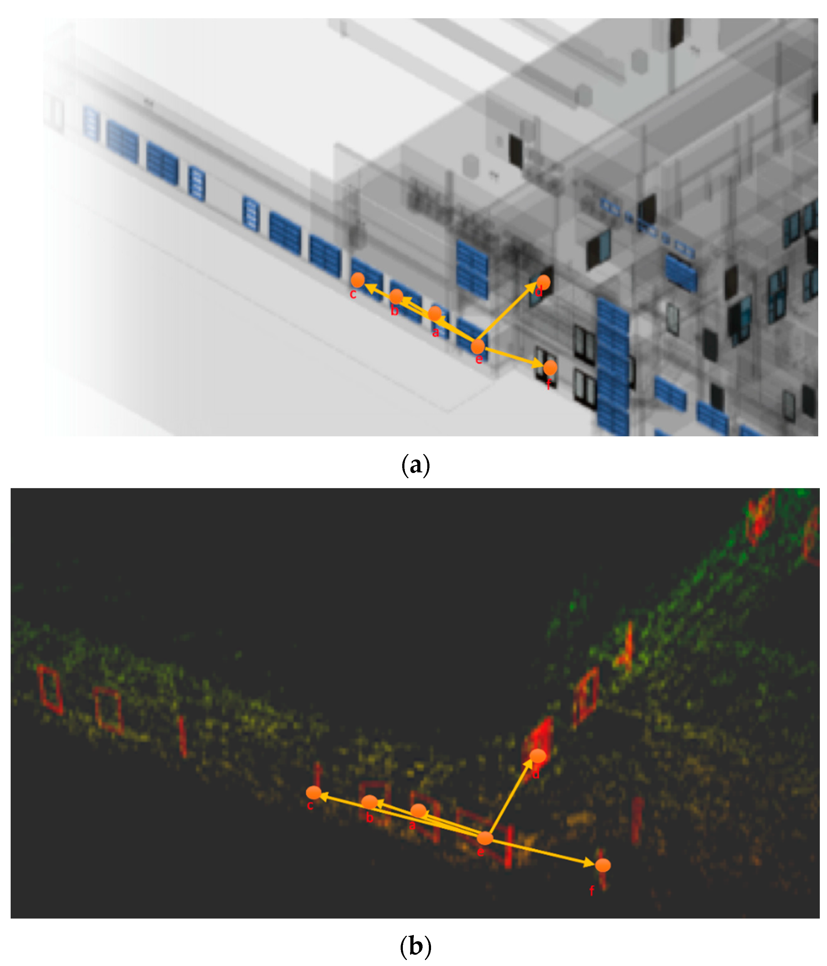
2.3. Macro-Feature Registeration and Matching

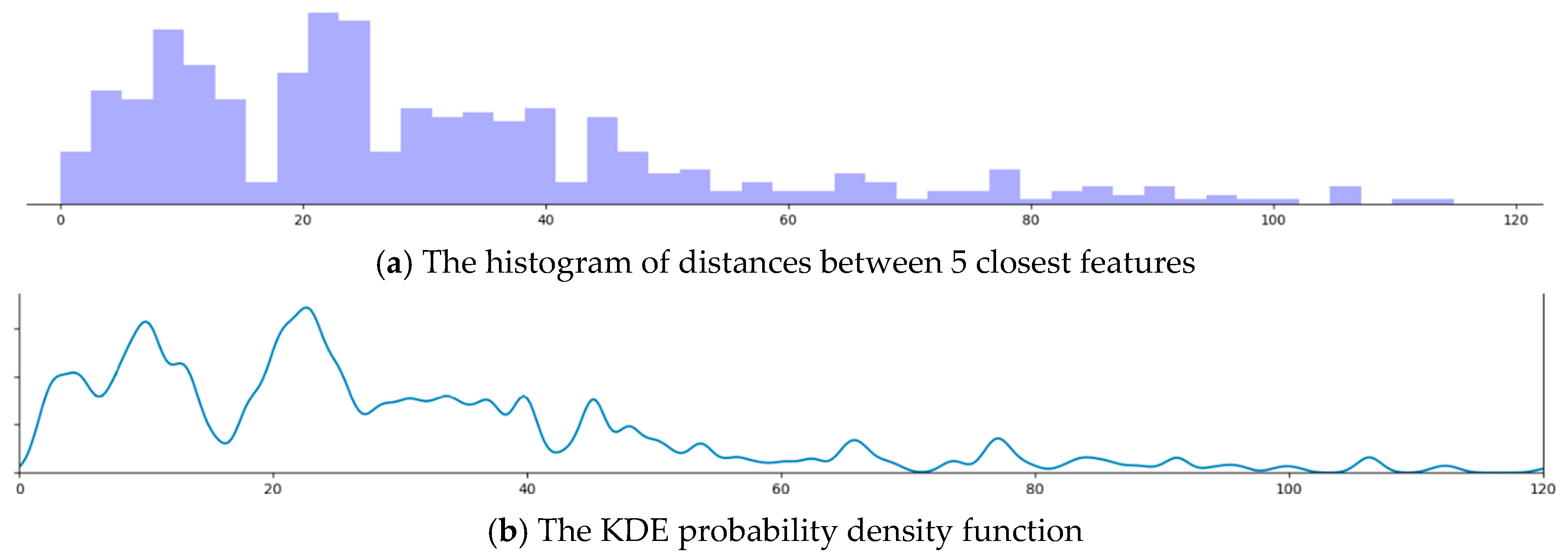
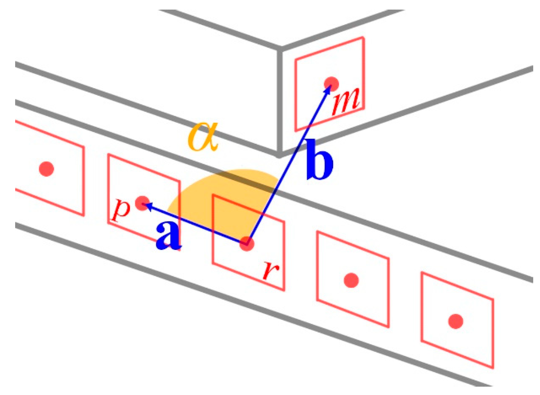
2.3.1. Lookup Table and Vector Structure
2.3.2. Initial Registration
3. Hardware Implementation
3.1. Preprocessing
3.2. Exploration Mode
3.3. Localized Mode
4. Experimental Results and Analysis
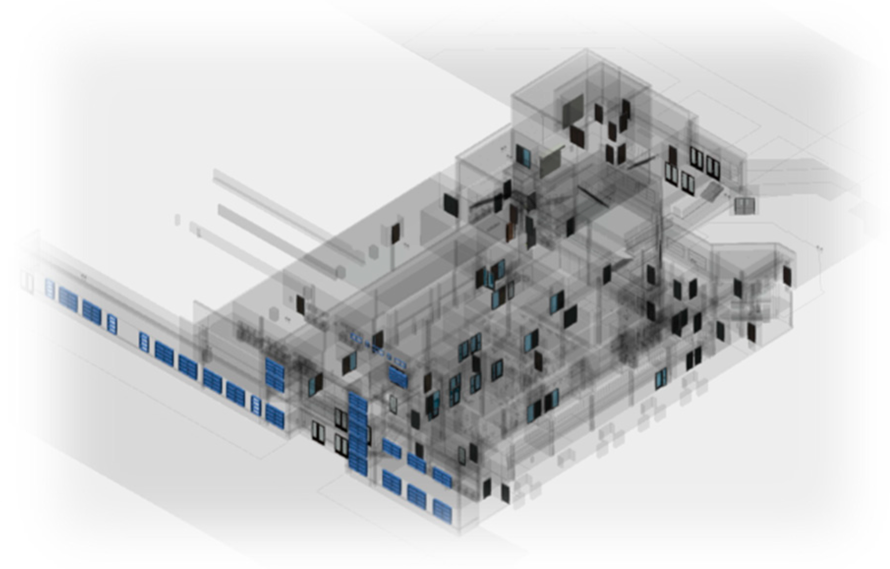
4.1. Object Vector Results and Accuracy
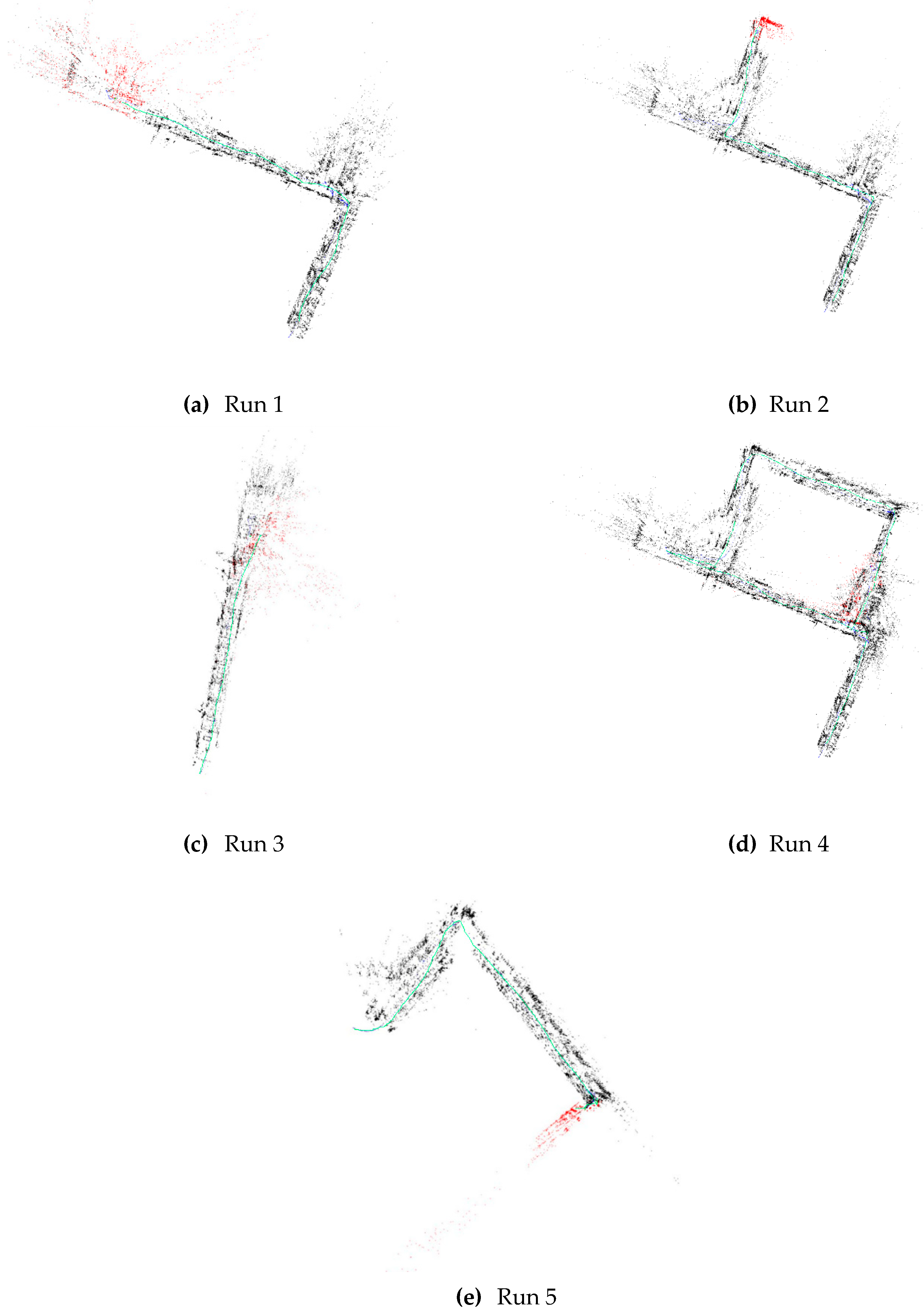
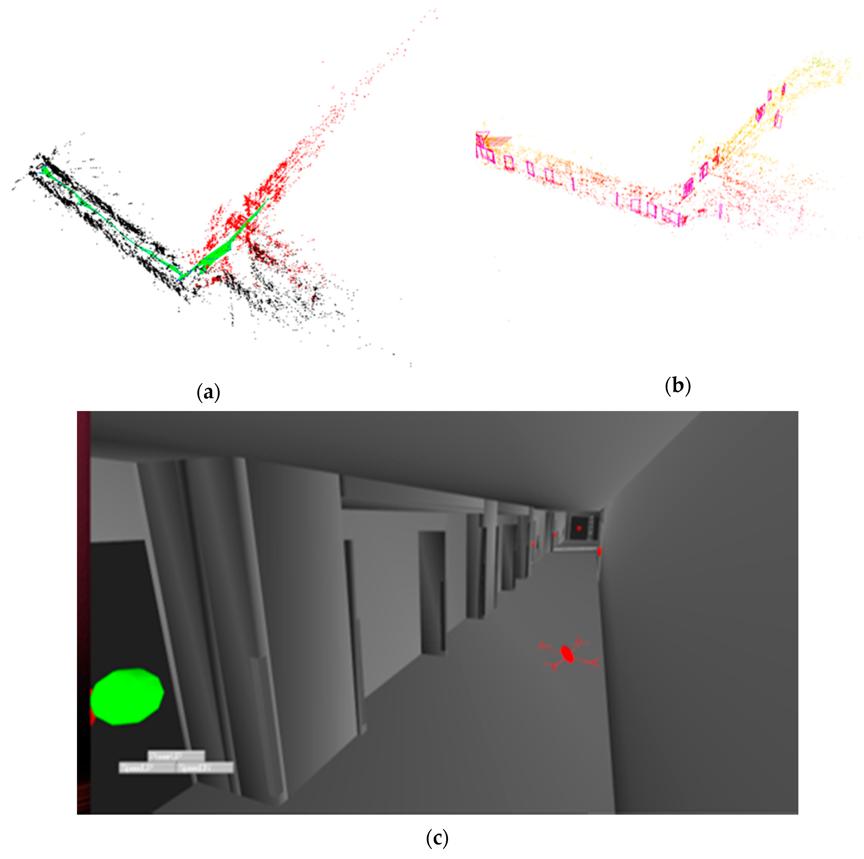
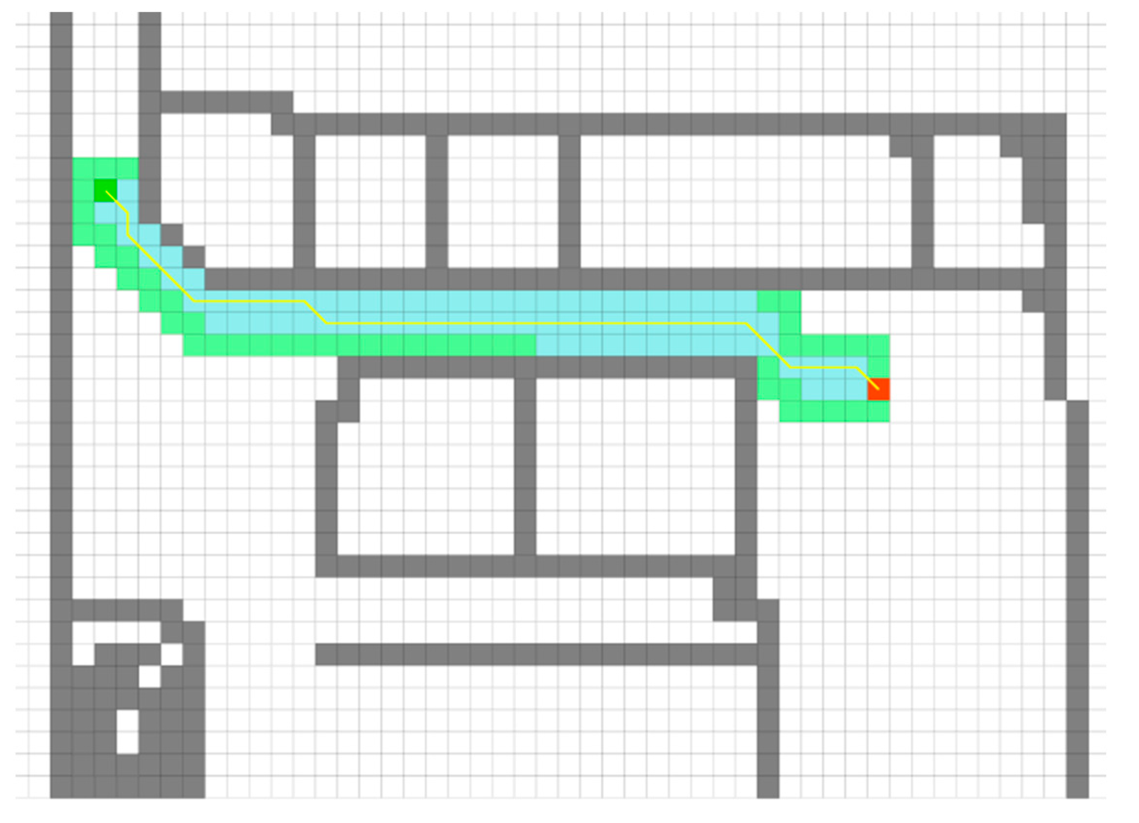
4.2. Localization within the CAD Model
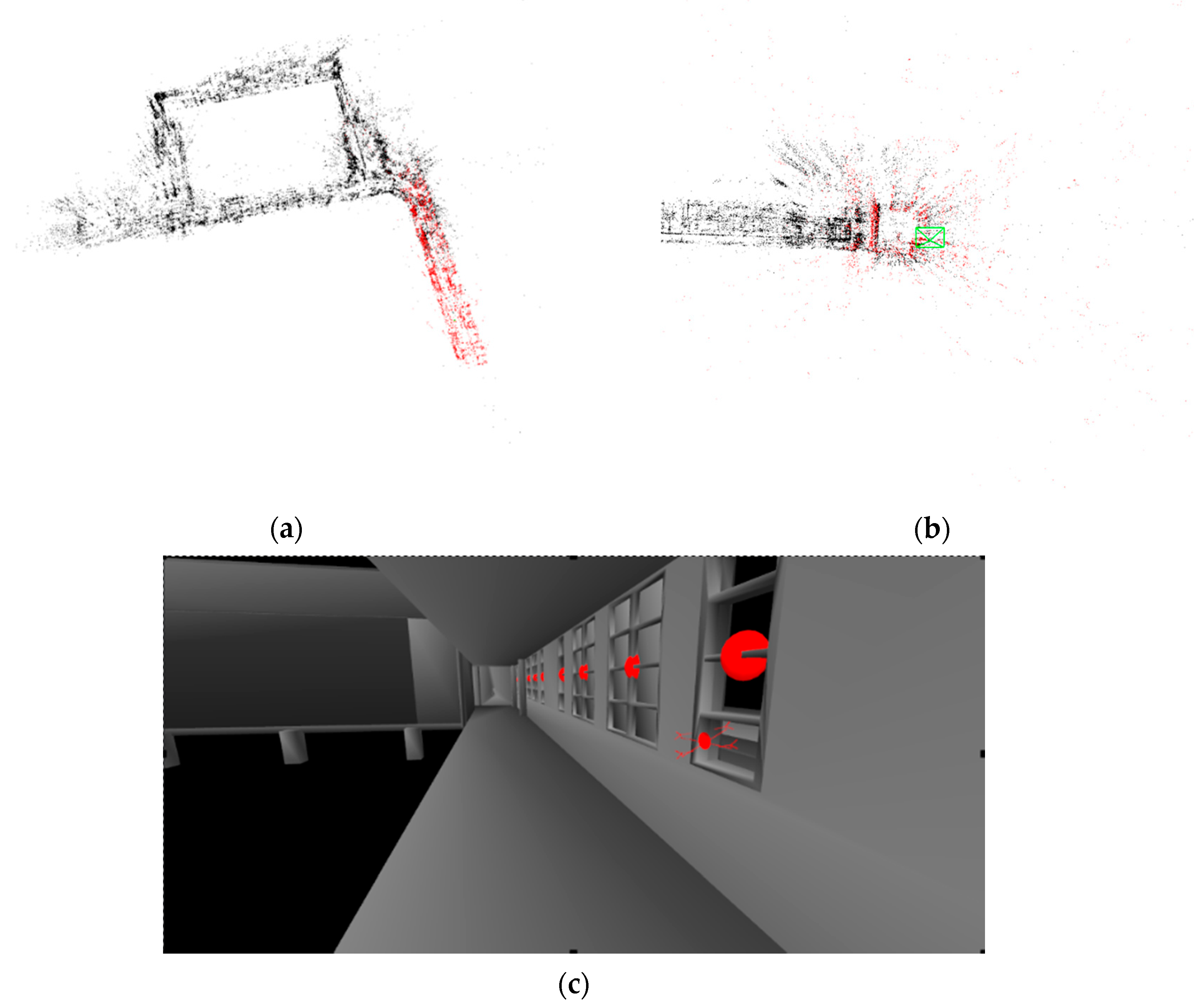
4.3. Re-Localization within the CAD Model
5. Conclusions
Future Work
Supplementary Materials
Author Contributions
Funding
Conflicts of Interest
References
- Lee, J.Y.; Chung, A.Y.; Shim, H.; Joe, C.; Park, S.; Kim, H. UAV Flight and Landing Guidance System for Emergency Situations. Sensors 2019, 19, 4468. [Google Scholar] [CrossRef] [PubMed] [Green Version]
- Nguyen, D.D.; Elouardi, A.; Florez, S.A.R.; Bouaziz, S. HOOFR SLAM System: An Embedded Vision SLAM Algorithm and Its Hardware-Software Mapping-Based Intelligent Vehicles Applications. IEEE Trans. Intell. Transp. Syst. 2019, 20, 4103–4118. [Google Scholar] [CrossRef]
- Padhy, R.P.; Verma, S.; Ahmad, S.; Choudhury, S.K.; Sa, P.K. Deep Neural Network for Autonomous UAV Navigation in Indoor Corridor Environments. Procedia Comput. Sci. 2018, 133, 643–650. [Google Scholar] [CrossRef]
- Liu, H.; Darabi, H.; Banerjee, P.; Liu, J. Survey of Wireless Indoor Positioning Techniques and Systems. IEEE Trans. Syst. Man Cybern. Part C Appl. Rev. 2017, 37, 1067–1080. [Google Scholar] [CrossRef]
- Montanha, A.; Polidorio, A.M.; Dominguez-Mayo, F.J.; Escalona, M.J. 2D Triangulation of Signals Source by Pole-Polar Geometric Models. Sensors 2019, 19, 1020. [Google Scholar] [CrossRef] [Green Version]
- Oliveria, L.; Di Franco, C.; Aburdan, T.E.; Almeida, L. Fusing Time-of-Flight and Received Signal Strength for adaptive radio-frequency ranging. In Proceedings of the 16th International Conference on Advanced Robotics (ICAR), Montevideo, Uruguay, 25–29 November 2013; pp. 1–6. [Google Scholar]
- Fraga-Lamas, P.; Ramos, L.; Mondéjar-Guerra, V.; Fernández-Caramés, T.M. A Review on IoT Deep Learning UAV Systems for Autonomous Obstacle Detection and Collision Avoidance. Remote Sens. 2019, 11, 2144. [Google Scholar] [CrossRef] [Green Version]
- Koch, O.; Teller, S. Wide-Area Egomotion Estimation from Known 3D Structure. In Proceedings of the IEEE Conference on Computer Vision and Pattern Recognition, Minneapolis, MN, USA, 17–22 June 2007; pp. 1–8. [Google Scholar]
- Li-Chee-Ming, J.; Armenakis, C. UAV navigation system using line-based sensor pose estimation. Geo Spat. Inf. Sci. 2018, 21, 2–11. [Google Scholar] [CrossRef] [Green Version]
- Engel, J.; Schöps, T.; Cremers, D. LSD-SLAM: Large-Scale Direct Monocular SLAM. In Proceedings of the European Conference on Computer Vision, Zurich, Switzerland, 6–12 September 2014; pp. 834–849. [Google Scholar]
- Hasan, A.; Qadir, A.; Nordeng, I.; Neubert, J. Construction Inspection through Spatial Database. In Proceedings of the 34rd International Association for Automation and Robotics in Construction, Taipei, Taiwan, 28 June–1 July 2017; pp. 840–847. [Google Scholar]
- Pătrăucean, V.; Armeni, I.; Nahangi, M.; Yeung, J.; Brilakis, I.; Haas, C. State of research in automatic as-built modelling. Adv. Eng. Inf. 2015, 29, 162–171. [Google Scholar] [CrossRef] [Green Version]
- Zhang, H.; Wu, J.; Liu, Y.; Yu, J. VaryBlock: A Novel Approach for Object Detection in Remote Sensed Images. Sensors 2019, 19, 5284. [Google Scholar] [CrossRef] [Green Version]
- Li, S.; Niu, Y.; Feng, C.; Liu, H.; Zhang, D.; Qin, H. An Onsite Calibration Method for MEMS-IMU in Building Mapping Fields. Sensors 2019, 19, 4150. [Google Scholar] [CrossRef] [Green Version]
- Assimp: Open Asset Import Library. Available online: http://www.assimp.org (accessed on 11 December 2019).
- Arya, S.; Mount, D.M.; Netanyahu, N.S.; Silverman, R.; Wu, A.Y. An optimal algorithm for approximate nearest neighbor searching fixed dimensions. J. ACM 1998, 45, 891–923. [Google Scholar] [CrossRef] [Green Version]
- Anzola, J.; Pascual, J.; Tarazona, G.; González Crespo, R. A Clustering WSN Routing Protocol Based on k-d Tree Algorithm. Sensors 2018, 18, 2899. [Google Scholar] [CrossRef] [PubMed] [Green Version]
- Tzutalin. LabelImg. Git Code. 2015. Available online: https://github.com/tzutalin/labelImg (accessed on 11 December 2019).
- Von Gioi, R.G.; Jakubowicz, J.; Morel, J.M.; Randall, G. LSD: A fast line segment detector with a false detection control. IEEE Trans. Pattern Anal. Mach. Intell. 2010, 32, 722–732. [Google Scholar] [CrossRef] [PubMed]
- Sun, Y.; Wang, Q.; Tansey, K.; Ullah, S.; Liu, F.; Zhao, H.; Yan, L. Multi-Constrained Optimization Method of Line Segment Extraction Based on Multi-Scale Image Space. ISPRS Int. J. Geo Inf. 2019, 8, 183. [Google Scholar] [CrossRef] [Green Version]
- Derpanis, K.G. Overview of the RANSAC Algorithm. Image Rochester NY 2010, 4, 2–3. [Google Scholar]
- Elgammal, A.; Harwood, D.; Davis, L. Non-parametric Model for Background Subtraction. In Proceedings of the 6th European Conference on Computer Vision-Part II, Dublin, Ireland, 26 June–1 July 2000; pp. 751–767. [Google Scholar]
- Hirschmuller, H. Stereo Processing by Semiglobal Matching and Mutual Information. IEEE Trans. Pattern Anal. Mach. Intell. 2007, 30, 328–341. [Google Scholar] [CrossRef]
- Quigley, M.; Conley, K.; Gerkey, B.; Faust, J.; Foote, T.; Leibs, J.; Wheeler, R.; Ng, A.Y. ROS: An open-source Robot Operating System. In Proceedings of the ICRA Workshop on Open Source Software, Kobe, Japan, 17 May 2009; p. 5. [Google Scholar]
- Mur-Artal, R.; Tardós, J.D. Orb-slam2: An open-source slam system for monocular, stereo, and rgb-d cameras. IEEE Trans. Robot. 2017, 33, 1255–1262. [Google Scholar] [CrossRef] [Green Version]
- Qin, J.; Li, M.; Liao, X.; Zhong, J. Accumulative Errors Optimization for Visual Odometry of ORB-SLAM2 Based on RGB-D Cameras. ISPRS Int. J. Geo Inf. 2019, 8, 581. [Google Scholar] [CrossRef] [Green Version]
- Wurm, K.M.; Hornung, A.; Bennewitz, M.; Stachniss, C.; Burgard, W. OctoMap: A probabilistic, flexible, and compact 3D map representation for robotic systems. In Proceedings of the ICRA 2010 Workshop on Best Practice in 3D Perception and Modeling for Mobile Manipulation, Anchorage, AK, USA, 3–7 May 2010; pp. 403–412. [Google Scholar]
- Faria, M.; Ferreira, A.S.; Pérez-Leon, H.; Maza, I.; Viguria, A. Autonomous 3D Exploration of Large Structures Using an UAV Equipped with a 2D LIDAR. Sensors 2019, 19, 4849. [Google Scholar] [CrossRef] [Green Version]
- Zhang, H.; Li, M.; Yang, L. Safe Path Planning of Mobile Robot Based on Improved A* Algorithm in Complex Terrains. Algorithms 2018, 11, 44. [Google Scholar] [CrossRef] [Green Version]
- Olson, E. AprilTag: A robust and flexible visual fiducial system. In Proceedings of the 2011 IEEE International Conference on Robotics and Automation, Shanghai, China, 9–13 May 2011; pp. 3400–3407. [Google Scholar]
- Abbas, S.M.; Aslam, S.; Berns, K.; Muhammad, A. Analysis and Improvements in AprilTag Based State Estimation. Sensors 2019, 19, 5480. [Google Scholar] [CrossRef] [PubMed] [Green Version]


| Run Id | Features Detected | Correct Matches | Incorrect Matched | Accuracy |
|---|---|---|---|---|
| Run 1 | 21 | 15 | 6 | 71.4% |
| Run 2 | 25 | 19 | 6 | 76% |
| Run 3 | 7 | 4 | 3 | 57.1% |
| Run 4 | 31 | 24 | 7 | 77.4% |
| Run 5 | 19 | 14 | 5 | 73.6% |
| Run Id | Localization Time (s) | Error (m) | Error (% of Trajectory Length) |
|---|---|---|---|
| Run 1 | 16 | 0.25 | 4% |
| Run 2 | 17 | 0.14 | 3% |
| Run 3 | 13 | 0.23 | 3% |
| Run 4 | 15 | 0.15 | 1% |
| Run 5 | 13 | 0.26 | 2% |
© 2020 by the authors. Licensee MDPI, Basel, Switzerland. This article is an open access article distributed under the terms and conditions of the Creative Commons Attribution (CC BY) license (http://creativecommons.org/licenses/by/4.0/).
Share and Cite
Haque, A.; Elsaharti, A.; Elderini, T.; Elsaharty, M.A.; Neubert, J. UAV Autonomous Localization Using Macro-Features Matching with a CAD Model. Sensors 2020, 20, 743. https://doi.org/10.3390/s20030743
Haque A, Elsaharti A, Elderini T, Elsaharty MA, Neubert J. UAV Autonomous Localization Using Macro-Features Matching with a CAD Model. Sensors. 2020; 20(3):743. https://doi.org/10.3390/s20030743
Chicago/Turabian StyleHaque, Akkas, Ahmed Elsaharti, Tarek Elderini, Mohamed Atef Elsaharty, and Jeremiah Neubert. 2020. "UAV Autonomous Localization Using Macro-Features Matching with a CAD Model" Sensors 20, no. 3: 743. https://doi.org/10.3390/s20030743
APA StyleHaque, A., Elsaharti, A., Elderini, T., Elsaharty, M. A., & Neubert, J. (2020). UAV Autonomous Localization Using Macro-Features Matching with a CAD Model. Sensors, 20(3), 743. https://doi.org/10.3390/s20030743