Contribution to Speeding-Up the Solving of Nonlinear Ordinary Differential Equations on Parallel/Multi-Core Platforms for Sensing Systems


Abstract
1. Introduction
2. Related Works
2.1. General Linear Methods
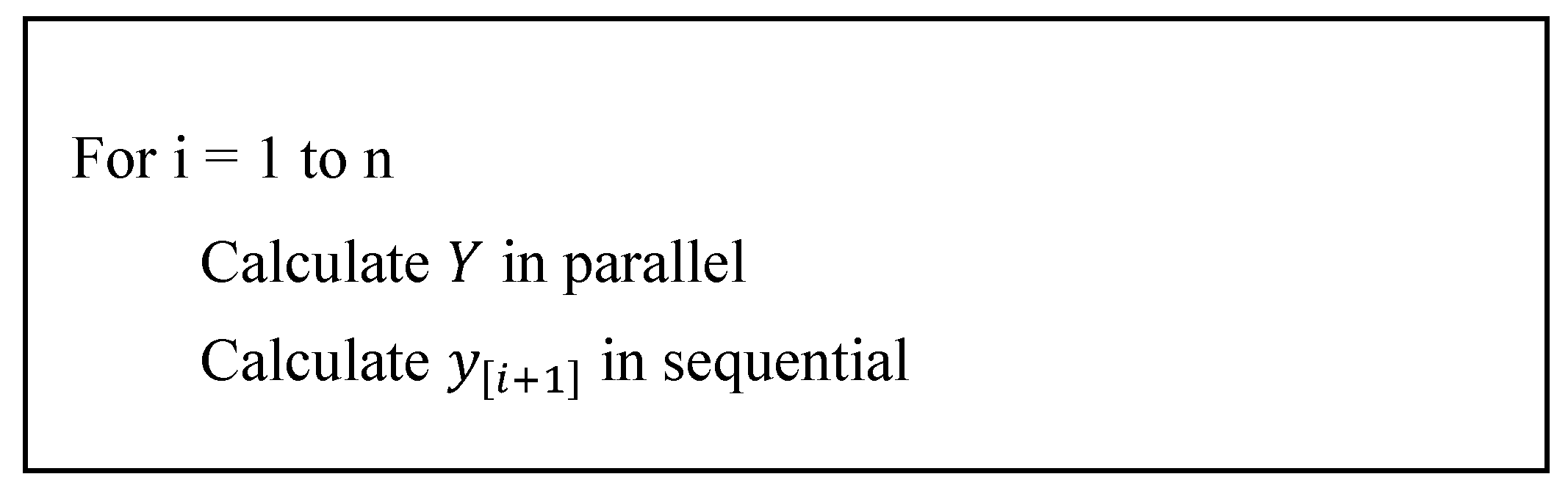
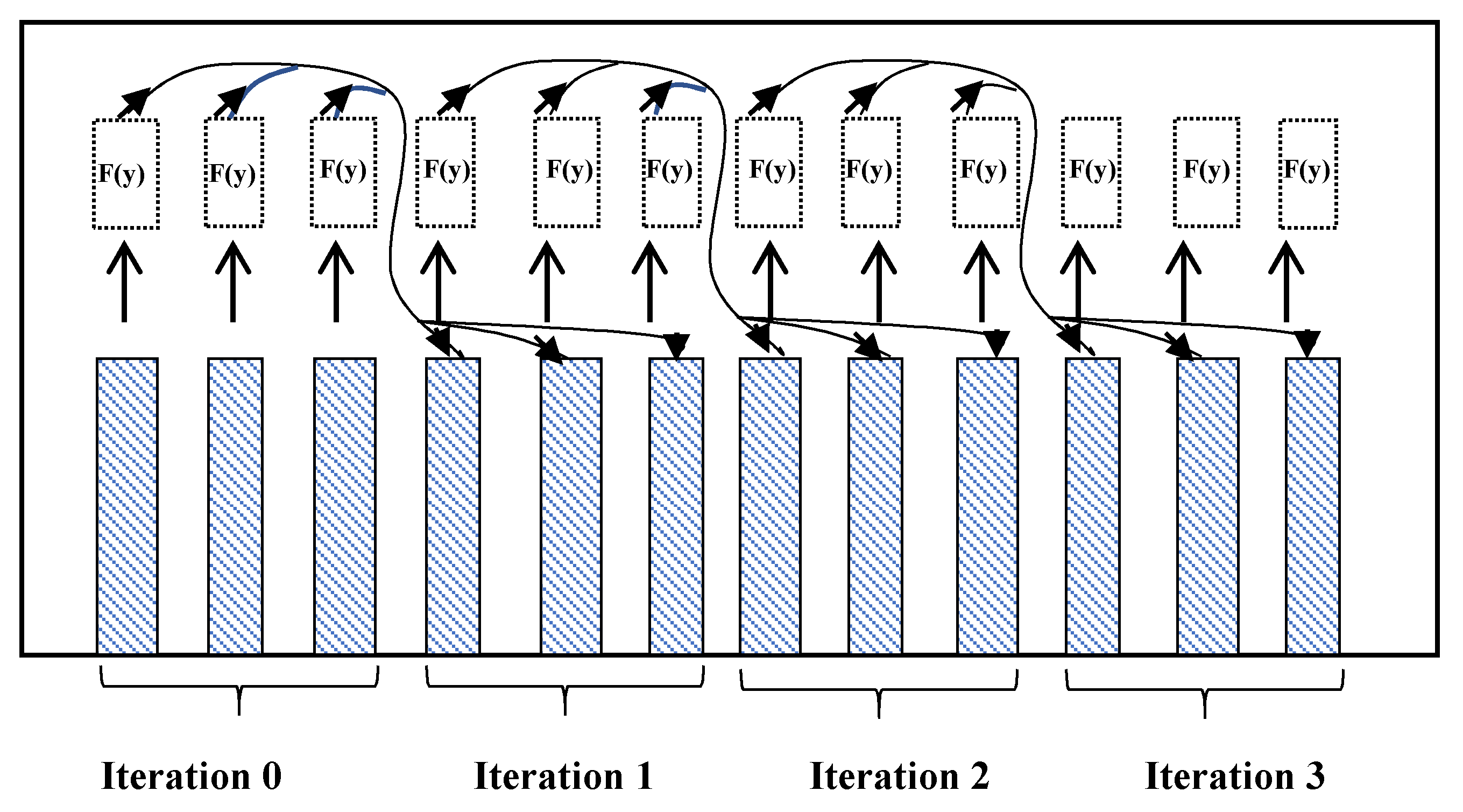
2.1.1. Parallel Iterated Runge-Kutta
2.1.2. Parallel Adams-Bashforth
2.2. Multiple Shotting Methods
- The “Coarse approximation,” which is with the initial conditions with the step size .
- The “Fine approximation,” which is with the initial conditions with the step size .
- Find the values of by using in a sequential way.
- Copy the values into in parallel.
- Find the values by using in parallel.
- Update in sequential with the following steps:
- .
- .
- Copy the values into .
- Go to the step 3 until you reach required precision.
2.3. Summary of the Main Previous/Traditional Methods
3. Our Novel Concept, the Parallel Adam-Moulton OpenCL
- Define the number of CPUs in group (g) based on current hardware restrictions.
- Define both work group step size and work item step size.
- Solve the starting points by using for example “DOPRI 5” and save them in , and their corresponding derivations as .
- Update in parallel through the following steps:
- Calculate the derivation F by using Equation (7), Equation (14) and save in .
- Wait for all values of , …, .
- Update the .
- Calculated the error for each computing unit and then update the global step size.
- Synchronize all computing units and update value in global variable.
- Go to the step 4 until all values calculated.
- (1)
- Calculating the gradient values for the next estimation points.
- (2)
- Transferring the gradient vectors into the global memory.
- (3)
- Estimating the next solution vector through an adapted Adams-Bashforth algorithm base on Equation (14) weights.
- (4)
- Calculate local truncation error to adjust the step-size.
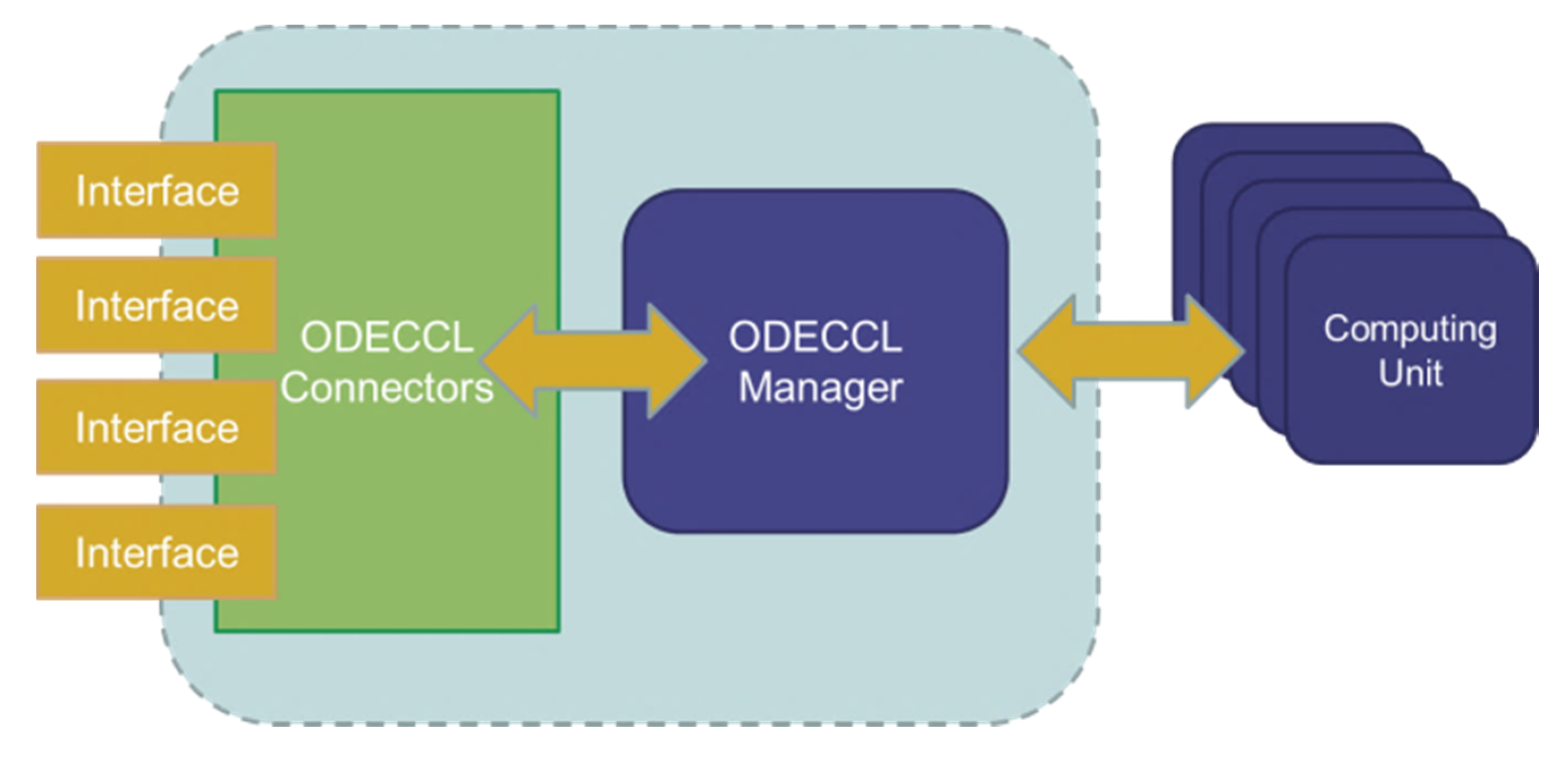
4. System Architecture
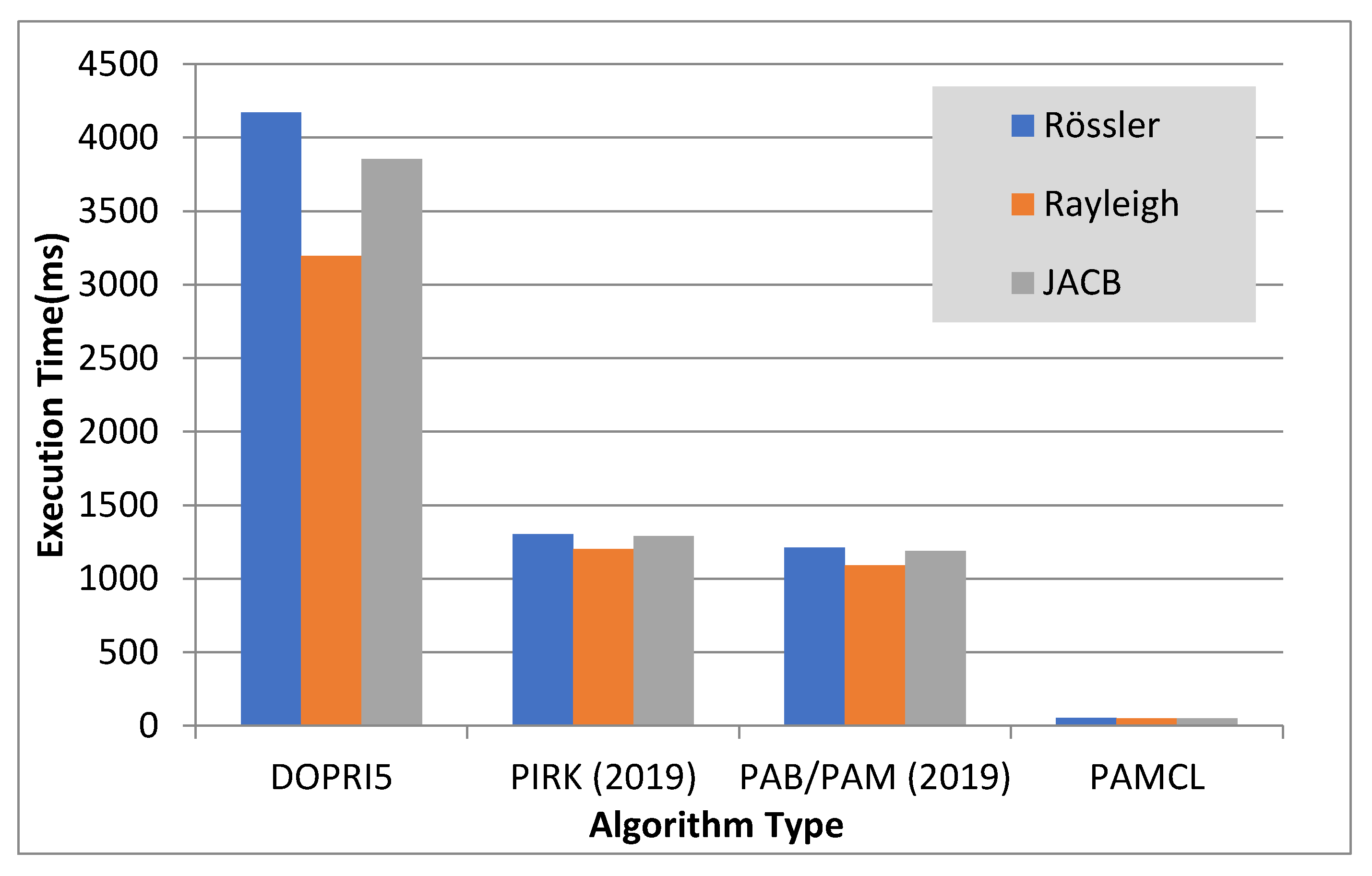
5. Numerical Experiments
6. Comparison of the Novel Concept (PAMCL) with Previous/Related Methods
7. Possible Extension of the PAMCL Model for also Solving PDE’s
- Converting PDE problem into ODE problem. Customize solver to solve PDE in parallel on n-CPUs/GPUs groups.
- Define the step-size of both coarse and fine estimators to find the solution of PDE between groups.
- Solving the PDE sequentially using the coarse estimator in the overall time span.
- Solving the PDE in parallel using fine estimator in each of the split time spans.
- Update the values in each of the split time spans by using the coarse estimator sequentially.
- Go to step 3 until we reach the required precision.
8. Conclusions
Author Contributions
Funding
Conflicts of Interest
References
- Sánchez-Garduño, F.; Pérez-Velázquez, J. Reactive-Diffusive-Advective Traveling Waves in a Family of Degenerate Nonlinear Equations. Sci. World J. 2016, 2016, 1–21. [Google Scholar] [CrossRef]
- Neumeyer, T.; Engl, G.; Rentrop, P. Numerical benchmark for the charge cycle in a combustion engine. Appl. Numer. Math. 1995, 18, 293–305. [Google Scholar] [CrossRef]
- Bajcinca, N.; Menarin, H.; Hofmann, S. Optimal control of multidimensional population balance systems for crystal shape manipulation. IFAC Proc. Vol. 2011, 44, 9842–9849. [Google Scholar] [CrossRef]
- Baumgartner, H.; Homburg, C. Applications of structural equation modeling in marketing and consumer research: A review. Int. J. Res. Mark. 1996, 13, 139–161. [Google Scholar] [CrossRef]
- Ilea, M.; Turnea, M.; Rotariu, M. Ordinary differential equations with applications in molecular biology. Rev. medico-chirurgicala a Soc. de Medici si Nat. din Iasi 2012, 116, 347–352. [Google Scholar]
- Yadav, M.; Malhotra, P.; Vig, L.; Sriram, K.; Shroff, G. ODE—Augmented Training Improves Anomaly Detection in Sensor Data from Machines. In Proceedings of the NIPS 2015 Time Series Workshop, Montreal, QC, Canada, 11 December 2015. [Google Scholar]
- Wang, X.; Li, C.; Song, D.-L.; Dean, R. A Nonlinear Circuit Analysis Technique for Time-Variant Inductor Systems. Sensors 2019, 19, 2321. [Google Scholar] [CrossRef] [PubMed]
- Mahmoodi, S.N.; Jalili, N.; Daqaq, M.F. Modeling, Nonlinear Dynamics, and Identification of a Piezoelectrically Actuated Microcantilever Sensor. IEEE/ASME Trans. Mechatron. 2008, 13, 58–65. [Google Scholar] [CrossRef]
- Omatu, S.; Soeda, T. Optimal Sensor Location in a Linear Distributed Parameter System. IFAC Proc. Vol. 1977, 10, 233–240. [Google Scholar] [CrossRef]
- Pérez-Velázquez, J.; Hense, B.A. Differential Equations Models to Study Quorum Sensing. Methods Mol. Biol. 2018, 1673, 253–271. [Google Scholar]
- Gander, M.J. Schawarz methods over the course of time. Electron. Trans. 2008, 31, 228–255. [Google Scholar]
- Gander, M.J. The origins of the alternating Schwarz method. In Domain Decomposition Methods in Science and Engineering XXI.; Springer: Berlin/Heidelberg, Germany, 2014; pp. 487–495. [Google Scholar]
- Niemeyer, K.E.; Sung, C.-J. GPU-Based Parallel Integration of Large Numbers of Independent ODE Systems. In Numerical Computations with GPUs; Springer: Berlin/Heidelberg, Germany, 2014; pp. 159–182. [Google Scholar]
- Liang, S.; Zhang, J.; Liu, X.-Z.; Hu, X.-D.; Yuan, W. Domain decomposition based exponential time differencing method for fluid dynamics problems with smooth solutions. Comput. Fluids 2019, 194. [Google Scholar] [CrossRef]
- Desai, A.; Khalil, M.; Pettit, C.; Poirel, D.; Sarkar, A. Scalable domain decomposition solvers for stochastic PDEs in high performance computing. Comput. Methods Appl. Mech. Eng. 2018, 335, 194–222. [Google Scholar] [CrossRef]
- Van Der Houwen, P.; Sommeijer, B.; Van Der Veen, W. Parallel iteration across the steps of high-order Runge-Kutta methods for nonstiff initial value problems. J. Comput. Appl. Math. 1995, 60, 309–329. [Google Scholar] [CrossRef][Green Version]
- Seen, W.M.; Gobithaasan, R.U.; Miura, K.T. GPU acceleration of Runge Kutta-Fehlberg and its comparison with Dormand-Prince method. AIP Conf. Proc. 2014, 1605, 16–21. [Google Scholar]
- Qin, Z.; Hou, Y. A GPU-Based Transient Stability Simulation Using Runge-Kutta Integration Algorithm. Int. J. Smart Grid Clean Energy 2013, 2, 32–39. [Google Scholar] [CrossRef]
- Pazner, W.; Persson, P.-O. Stage-parallel fully implicit Runge–Kutta solvers for discontinuous Galerkin fluid simulations. J. Comput. Phys. 2017, 335, 700–717. [Google Scholar] [CrossRef]
- Nievergelt, J. Parallel methods for intergrating ordinary differential equations. Commun. ACM 1964, 7, 731–733. [Google Scholar] [CrossRef]
- Wu, S.-L.; Zhou, T. Parareal algorithms with local time-integrators for time fractional differential equations. J. Comput. Phys. 2018, 358, 135–149. [Google Scholar] [CrossRef]
- Boonen, T.; Van Lent, J.; Vandewalle, S. An algebraic multigrid method for high order time-discretizations of the div-grad and the curl-curl equations. Appl. Numer. Math. 2009, 59, 507–521. [Google Scholar] [CrossRef]
- Carraro, T.; Friedmann, E.; Gerecht, D. Coupling vs decoupling approaches for PDE/ODE systems modeling intercellular signaling. J. Comput. Phys. 2016, 314, 522–537. [Google Scholar] [CrossRef]
- Bin Suleiman, M. Solving nonstiff higher order ODEs directly by the direct integration method. Appl. Math. Comput. 1989, 33, 197–219. [Google Scholar] [CrossRef]
- Van Der Houwen, P.; Messina, E. Parallel Adams methods. J. Comput. Appl. Math. 1999, 101, 153–165. [Google Scholar] [CrossRef][Green Version]
- Godel, N.; Schomann, S.; Warburton, T.; Clemens, M. GPU Accelerated Adams–Bashforth Multirate Discontinuous Galerkin FEM Simulation of High-Frequency Electromagnetic Fields. IEEE Trans. Magn. 2010, 46, 2735–2738. [Google Scholar] [CrossRef]
- Siow, C.; Koto, J.; Afrizal, E. Computational Fluid Dynamic Using Parallel Loop of Multi-Cores Processor. Appl. Mech. Mater. 2014, 493, 80–85. [Google Scholar] [CrossRef]
- Plaszewski, P.; Banas, K.; Maciol, P. Higher order FEM numerical integration on GPUs with OpenCL. In Proceedings of the International Multiconference on Computer Science and Information Technology, Wisla, Poland, 18–20 October 2010. [Google Scholar]
- Halver, R.; Homberg, W.; Sutmann, G. Benchmarking Molecular Dynamics with OpenCL on Many-Core Architectures. In Parallel Processing and Applied Mathematics; Springer: Cham, Switzerland, 2018. [Google Scholar]
- Rodriguez, M.; Blesa, F.; Barrio, R. OpenCL parallel integration of ordinary differential equations: Applications in computational dynamics. Comput. Phys. Commun. 2015, 192, 228–236. [Google Scholar] [CrossRef]
- Stone, C.P.; Davis, R.L. Techniques for Solving Stiff Chemical Kinetics on Graphical Processing Units. J. Propuls. Power 2013, 29, 764–773. [Google Scholar] [CrossRef]
- Markesteijn, A.; Karabasov, S.; Glotov, V.; Goloviznin, V. A new non-linear two-time-level Central Leapfrog scheme in staggered conservation–flux variables for fluctuating hydrodynamics equations with GPU implementation. Comput. Methods Appl. Mech. Eng. 2014, 281, 29–53. [Google Scholar] [CrossRef]
- Butcher, J. General linear methods. Comput. Math. Appl. 1996, 13, 105–112. [Google Scholar] [CrossRef]
- Van Der Veen, W.; De Swart, J.; Van Der Houwen, P. Convergence aspects of step-parallel iteration of Runge-Kutta methods. Appl. Numer. Math. 1995, 18, 397–411. [Google Scholar] [CrossRef]
- Fischer, M. Fast and parallel Runge--Kutta approximation of fractional evolution equations. SIAM J. Sci. Comput. 2019, 41, A927–A947. [Google Scholar] [CrossRef]
- Fathoni, M.F.; Wuryandari, A.I. Comparison between Euler, Heun, Runge-Kutta and Adams-Bashforth-Moulton integration methods in the particle dynamic simulation. In Proceedings of the 4th International Conference on Interactive Digital Media (ICIDM), Bandung, Indonesia, 1–5 December 2015. [Google Scholar]
- Bonchiş, C.; Kaslik, E.; Roşu, F. HPC optimal parallel communication algorithm for the simulation of fractional-order systems. J. Supercomput. 2019, 75, 1014–1025. [Google Scholar] [CrossRef]
- Saha, P.; Stadel, J.; Tremaine, S. A parallel intergration method for solar system dynamics. Astron. J. 1997, 114, 409–415. [Google Scholar] [CrossRef]
- Bellen, A.; Zennaro, M. Parallel algorithms for intial-value problems for difference and differential equations. J. Comput. Appl. Math. 1989, 25, 341–350. [Google Scholar] [CrossRef]
- Lions, J.; Maday, Y.; Turinici, G. A parareal in time descretization of PDEs. CR. Acad. Sci. Paris 2001, I, 661–668. [Google Scholar] [CrossRef]
- Cong, N.H. Continuous variable stepsize explicit pseudo two-step RK methods. J. Comput. Appl. Math. 1999, 101, 105–116. [Google Scholar] [CrossRef]
- Jaaskelainen, P.O.; De La Lama, C.S.; Huerta, P.; Takala, J.H. OpenCL-based Design Methodology for application-specific processors. In Proceedings of the 2010 International Conference on Embedded Computer Systems: Architectures, Modeling and Simulation, Samos, Greece, 19–22 July 2010. [Google Scholar]
- Gustafson, J.L. Reevaluating Amdahl’s law. Commun. ACM 1988, 31, 532–533. [Google Scholar] [CrossRef]
- Gander, M.J. 50 years of time parallel time integration. In Multiple Shooting and Time Domain Decomposition Methods; Springer: Berlin/Heidelberg, Germany, 2015. [Google Scholar]
- Wu, S.-L. A second-order parareal algorithm for fractional PDEs. J. Comput. Phys. 2016, 307, 280–290. [Google Scholar] [CrossRef]
- Pesch, H.J.; Bechmann, S.; Frey, M.; Rund, A.; Wurst, J.-E. Multiple Boundary-Value-Problem Formulation for PDE-constrained Optimal Control Problems with a Short History on Multiple Shooting for ODEs. 2013. Available online: https://eref.uni-bayreuth.de/4501 (accessed on 3 August 2020).


| Solver/Parameter | Work- Groups | Work Item | Kernel Type Number |
|---|---|---|---|
| PIRK | 1 | Depends on available cores | 1 |
| PAM | 1 | Depends on available cores | 1 |
| PAMCL | Variable | Depends on available cores divided by the number of Work-Groups | 2 * |
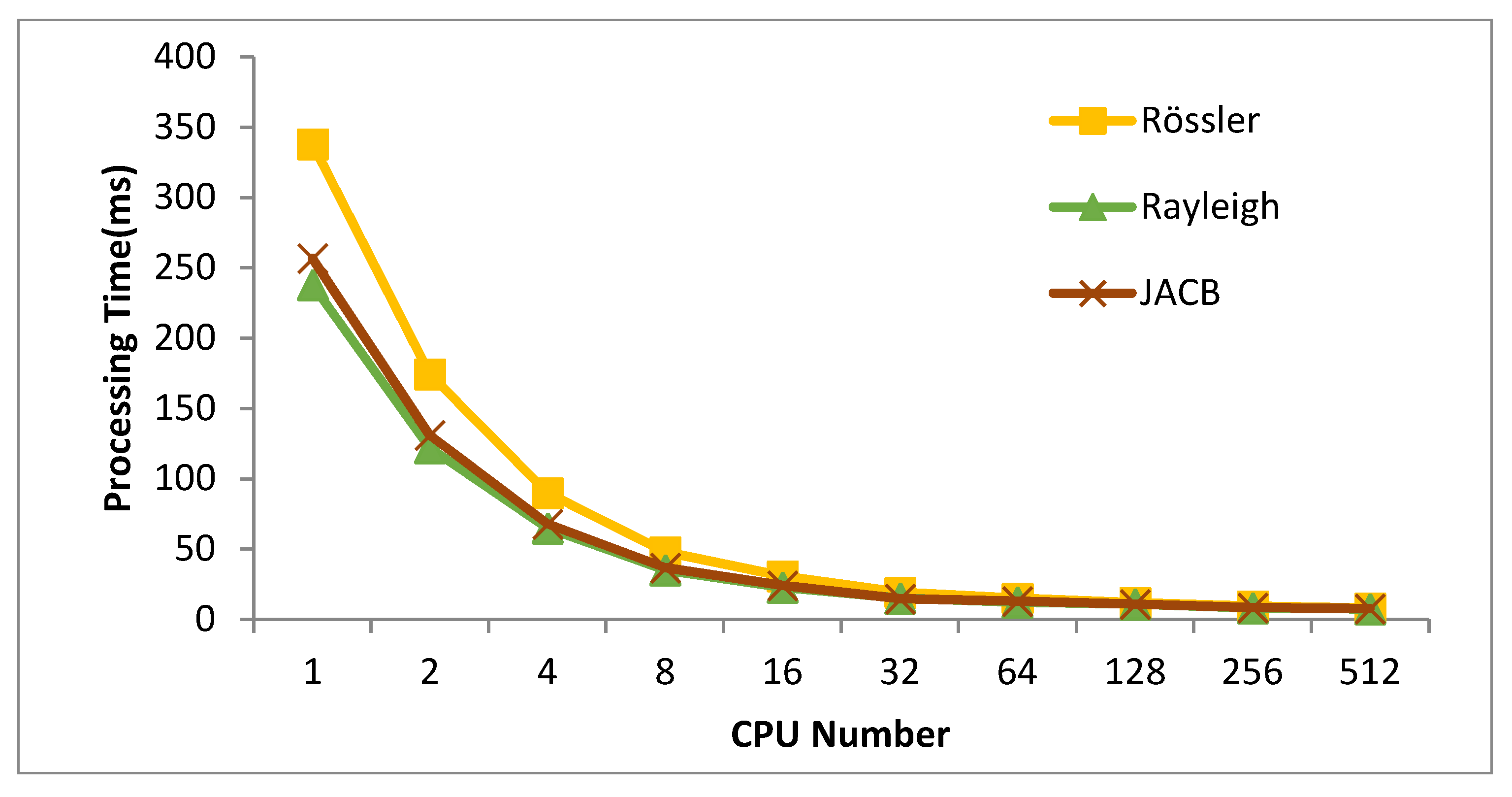
| Number of Cores on GPU | RAYLEIGH (ms) | JACB (ms) | RöSSLER (ms) |
|---|---|---|---|
| 1 | 238.0 | 257.1 | 338 |
| 2 | 122.0 | 131.1 | 174.46 |
| 8 | 35.0 | 36.7 | 48.1 |
| 64 | 12.4 | 13.1 | 15.2 |
| 512 | 7.4 | 7.8 | 8.5 |
| Method/ Algorithm | Error 0.01 | Error 0.001 | Error 0.0001 | |||
|---|---|---|---|---|---|---|
| Time (ms) on CPU | Speedup (i.e., on GPU) | Time (ms) on CPU | Speedup (i.e., on GPU) | Time (ms) on CPU | Speedup (i.e., on GPU) | |
| Dopri5 | 593.11 | 1x | 4171.01 | 1x | 41860.01 | 1x |
| PIRK (2019) | 169.23 | 3.50x | 1301.02 | 3.22x | 15013.89 | 2.79 |
| PAM/PAB (2019) | 129.12 | 4.26x | 1210.73 | 3.41x | 11540.44 | 3.62 |
| PAMCL | 6.93 | 69.43x | 51.83 | 80.47x | 439.82 | 95.17x |
| Method/ Algorithm | Error 0.01 | Error 0.001 | Error 0.0001 | |||
|---|---|---|---|---|---|---|
| Global Memory | Local Memory | Global Memory | Local Memory | Global Memory | Local Memory | |
| Dopri5 | 18 KB | 500 B | 200 KB | 500 B | 2.1 MB | 500 B |
| PIRK (2019) | 19 KB | 1.5 KB | 210 KB | 1.5 KB | 2.2 MB | 1.5 KB |
| PAM/PAB (2019) | 22 KB | 2.5 KB | 250 KB | 2.5 KB | 2.6 MB | 2.3 KB |
| PAMCL | 32 KB | 4 KB | 350 KB | 4 KB | 4.8 MB | 4 KB |
Publisher’s Note: MDPI stays neutral with regard to jurisdictional claims in published maps and institutional affiliations. |
© 2020 by the authors. Licensee MDPI, Basel, Switzerland. This article is an open access article distributed under the terms and conditions of the Creative Commons Attribution (CC BY) license (http://creativecommons.org/licenses/by/4.0/).
Share and Cite
Tavakkoli, V.; Mohsenzadegan, K.; Chedjou, J.C.; Kyamakya, K. Contribution to Speeding-Up the Solving of Nonlinear Ordinary Differential Equations on Parallel/Multi-Core Platforms for Sensing Systems. Sensors 2020, 20, 6130. https://doi.org/10.3390/s20216130
Tavakkoli V, Mohsenzadegan K, Chedjou JC, Kyamakya K. Contribution to Speeding-Up the Solving of Nonlinear Ordinary Differential Equations on Parallel/Multi-Core Platforms for Sensing Systems. Sensors. 2020; 20(21):6130. https://doi.org/10.3390/s20216130
Chicago/Turabian StyleTavakkoli, Vahid, Kabeh Mohsenzadegan, Jean Chamberlain Chedjou, and Kyandoghere Kyamakya. 2020. "Contribution to Speeding-Up the Solving of Nonlinear Ordinary Differential Equations on Parallel/Multi-Core Platforms for Sensing Systems" Sensors 20, no. 21: 6130. https://doi.org/10.3390/s20216130
APA StyleTavakkoli, V., Mohsenzadegan, K., Chedjou, J. C., & Kyamakya, K. (2020). Contribution to Speeding-Up the Solving of Nonlinear Ordinary Differential Equations on Parallel/Multi-Core Platforms for Sensing Systems. Sensors, 20(21), 6130. https://doi.org/10.3390/s20216130