A New In-Flight Alignment Method with an Application to the Low-Cost SINS/GPS Integrated Navigation System

Abstract
1. Introduction
2. Problem Formulation
2.1. Preliminary
2.2. Traditional Optimization-based Alignment Method
2.3. Problem Formulation
3. The Proposed IFA Method
3.1. Modified Construction Method of Double-Vectors
3.2. Fast IFA Method Mased on Gradient Descent
4. Simulation and Experiment Results
4.1. Simulation For the Proposed IFA Method
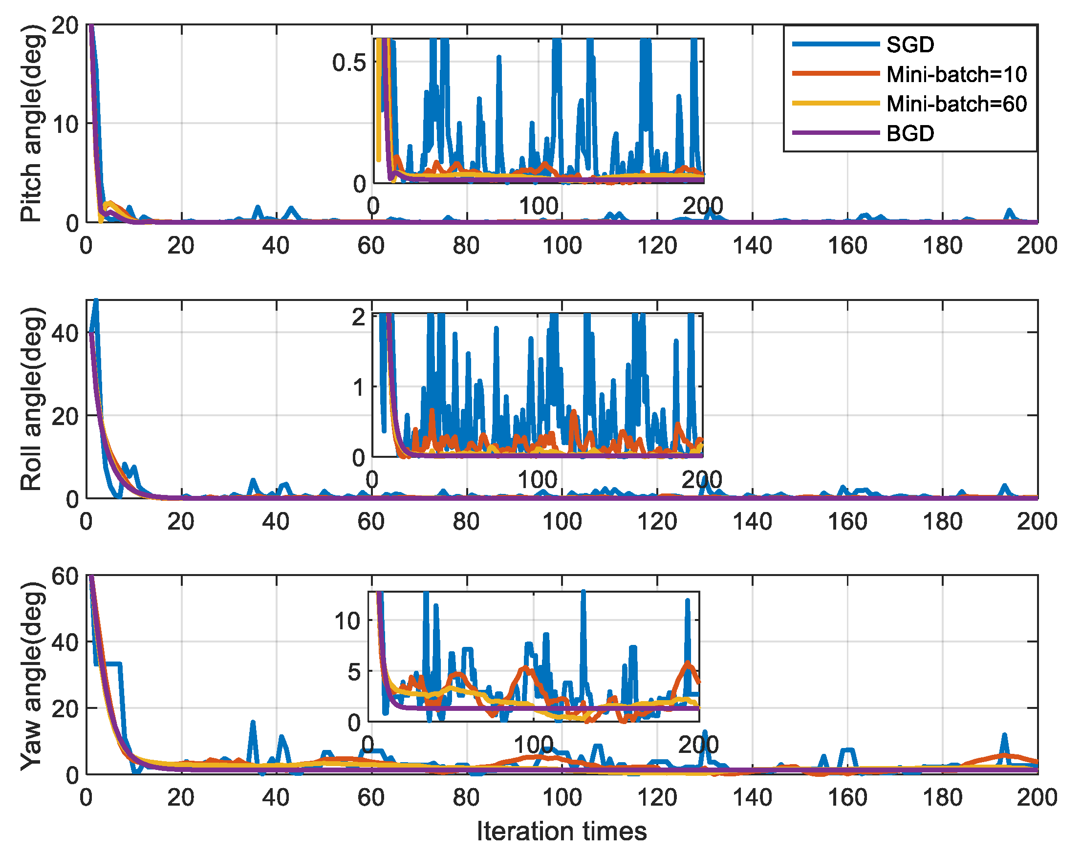
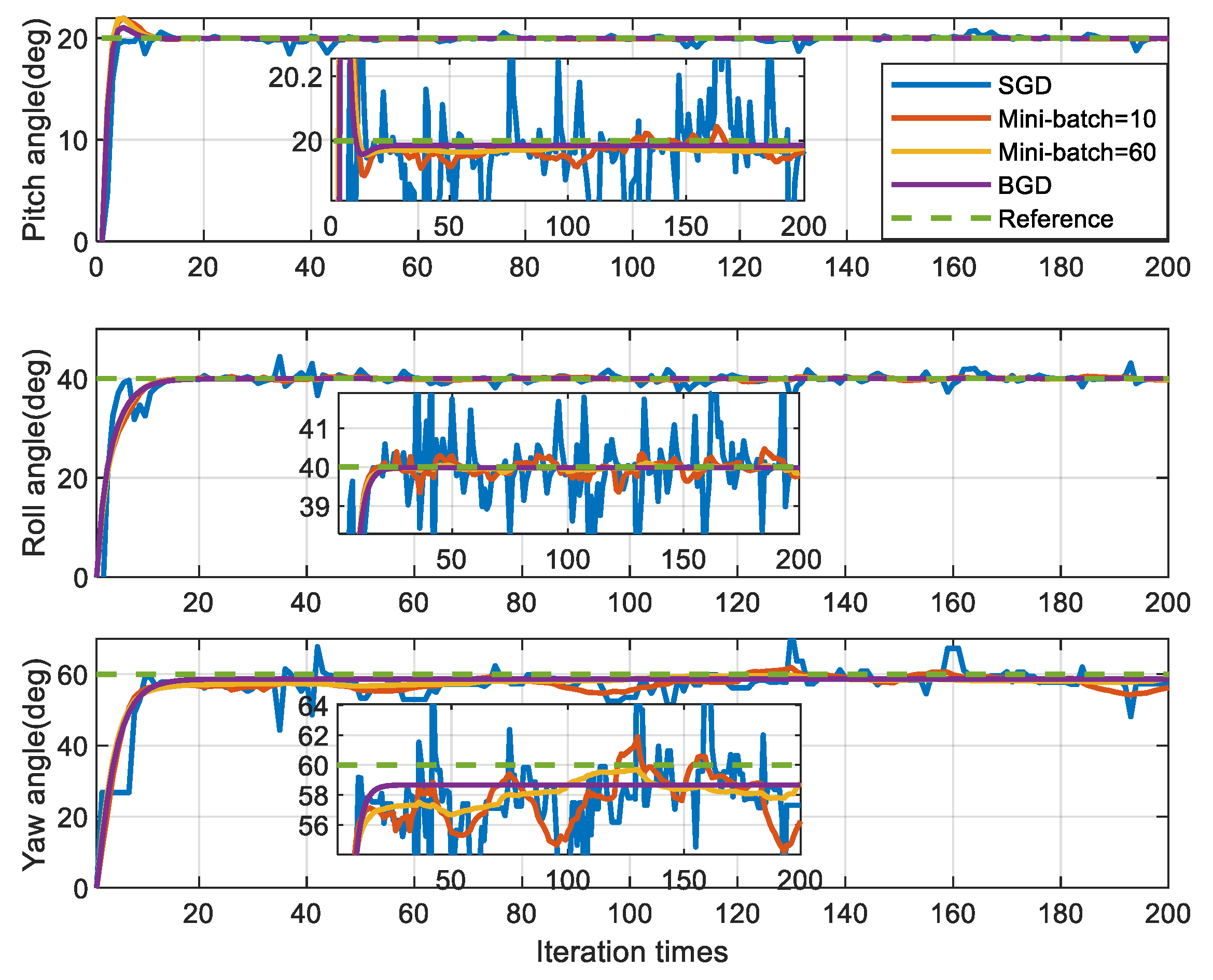
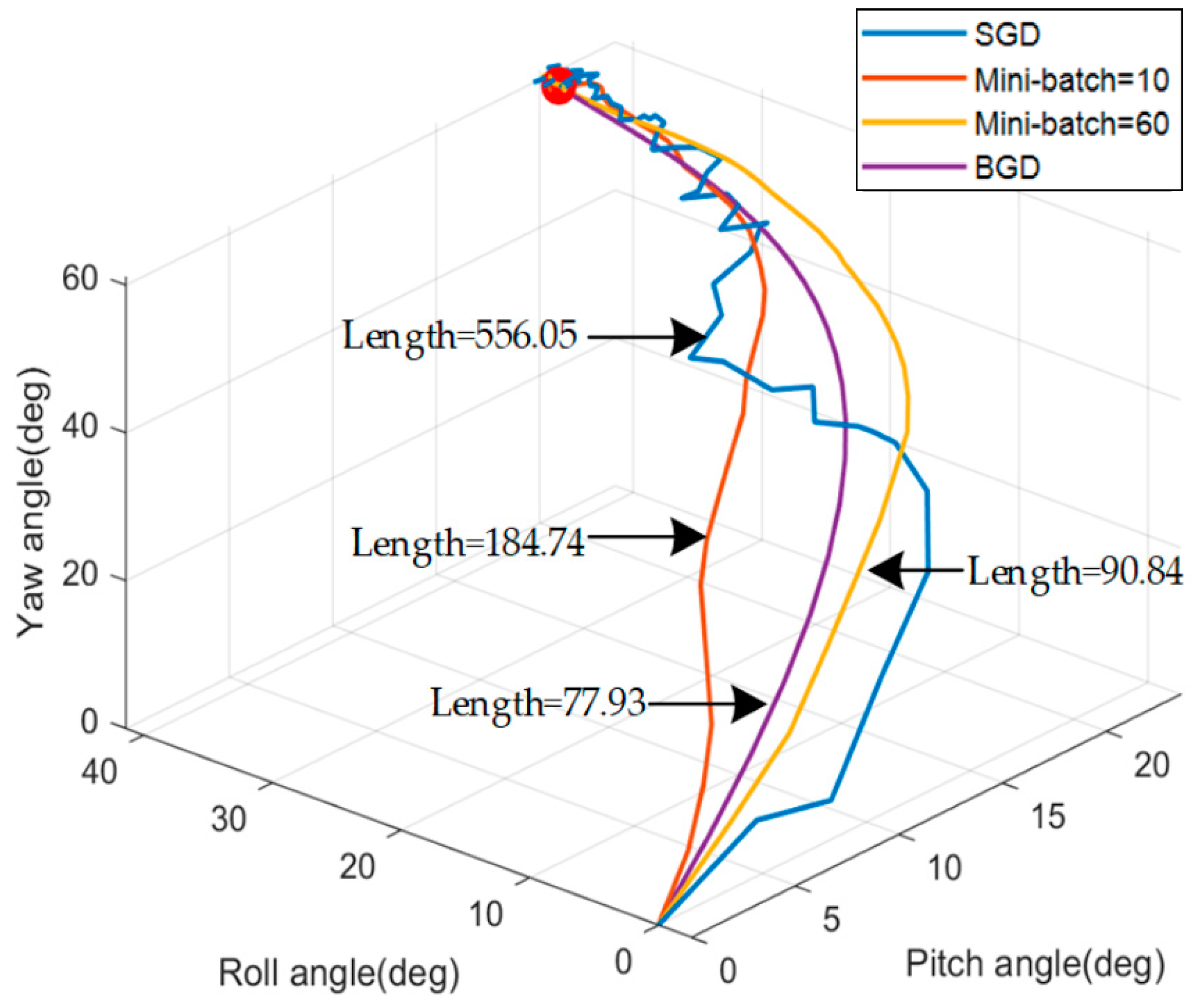
4.2. Simulation For Different Sizes of Mini-Batch
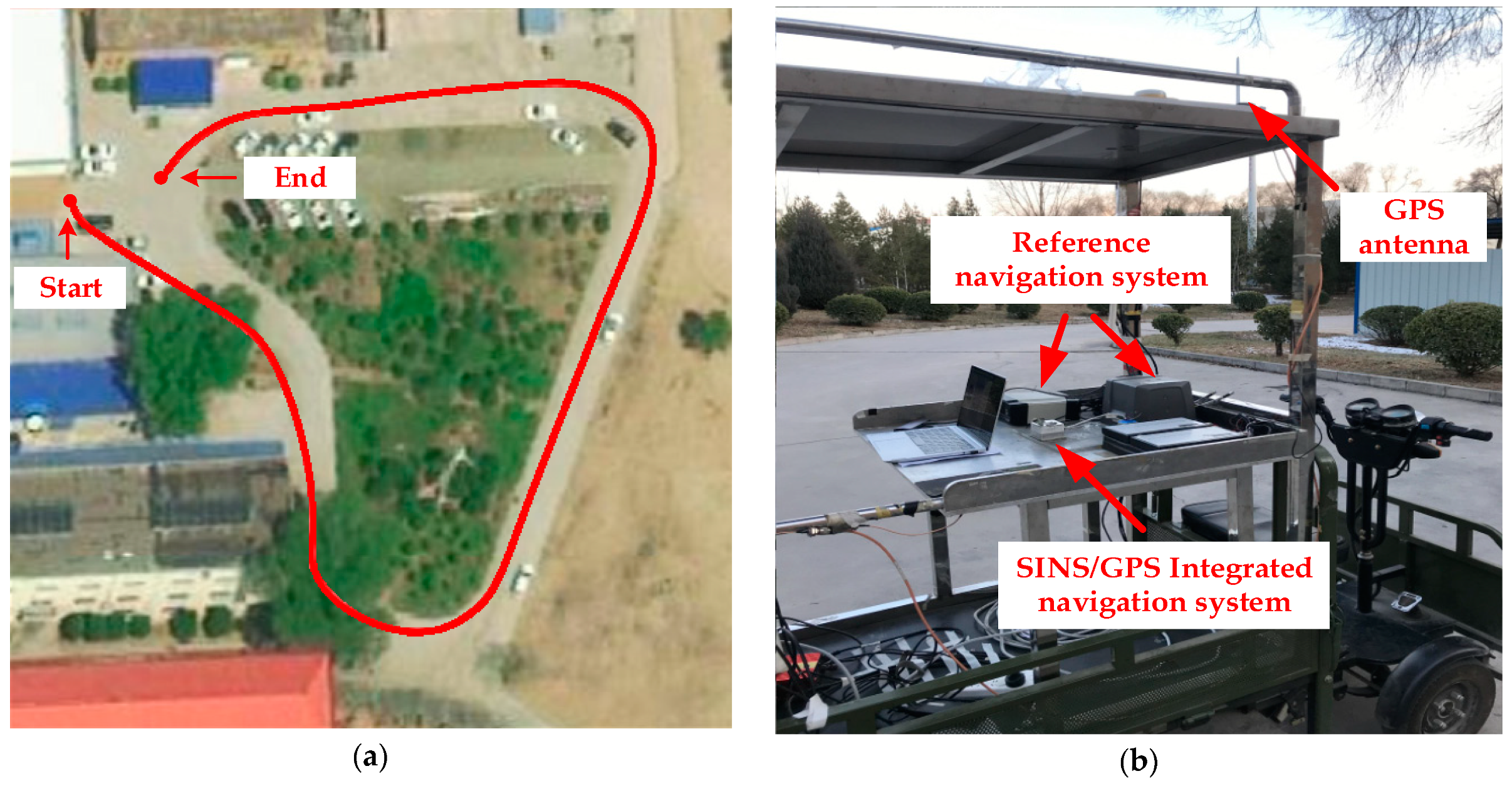
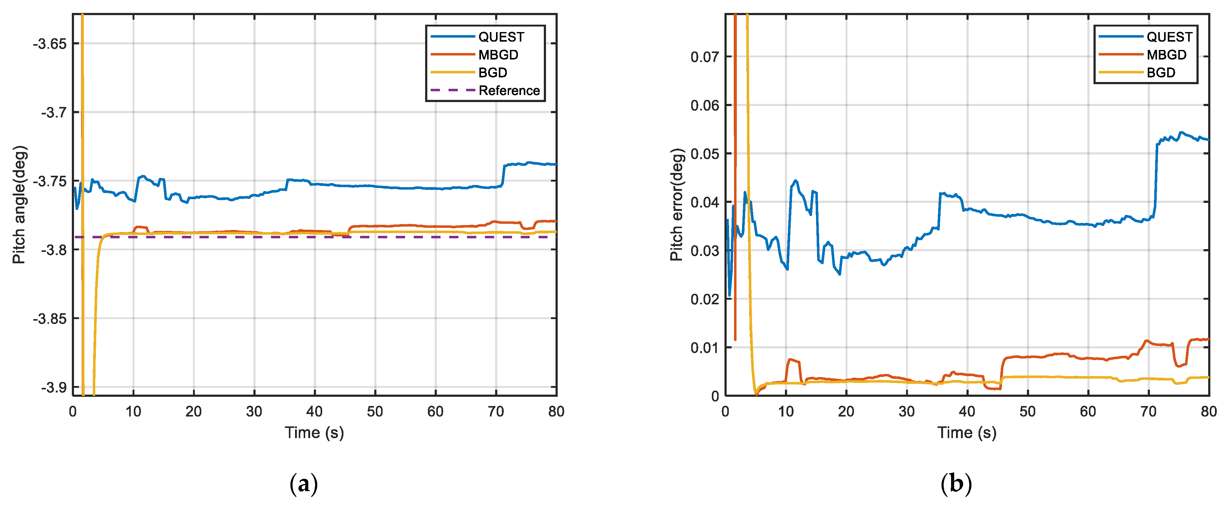
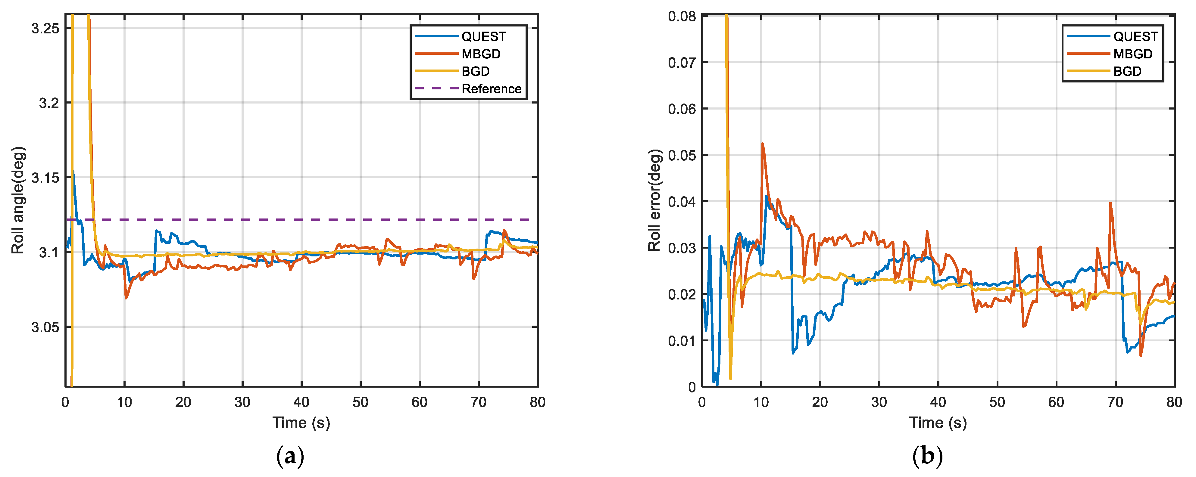
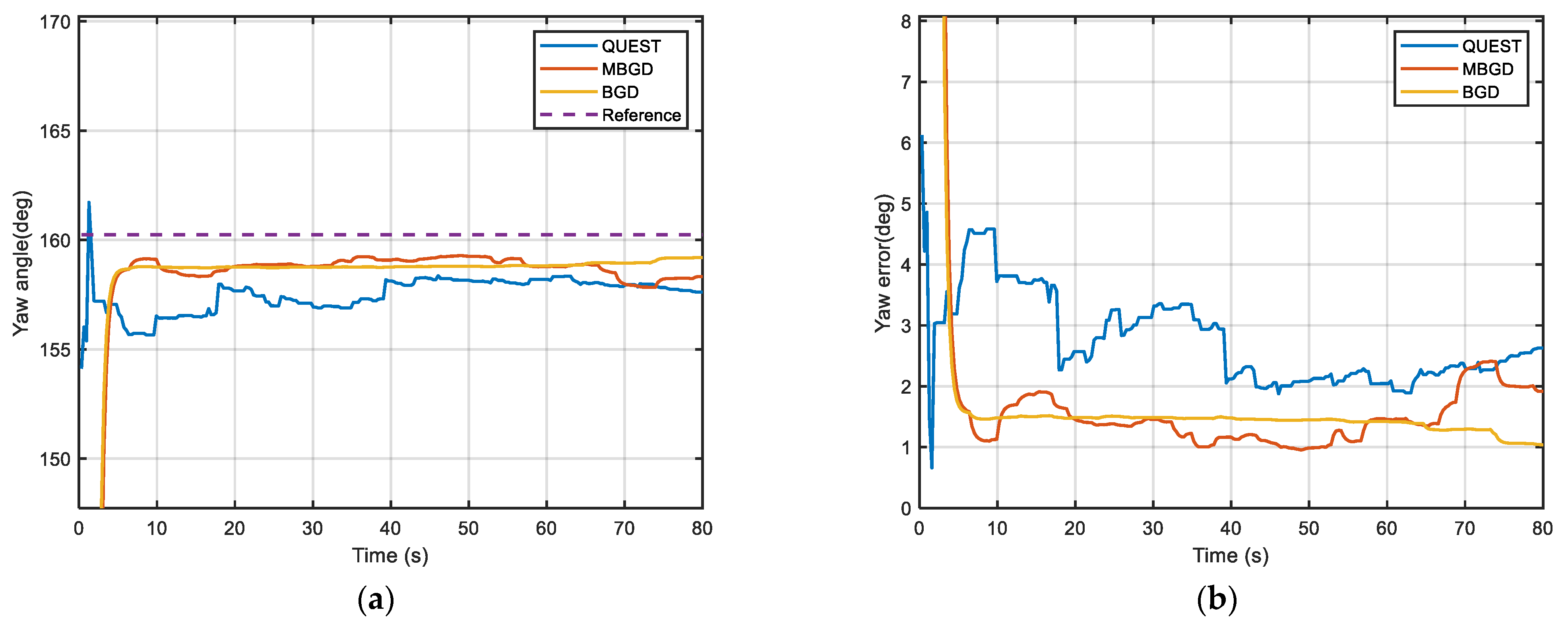
4.3. Experiment Results
5. Conclusions
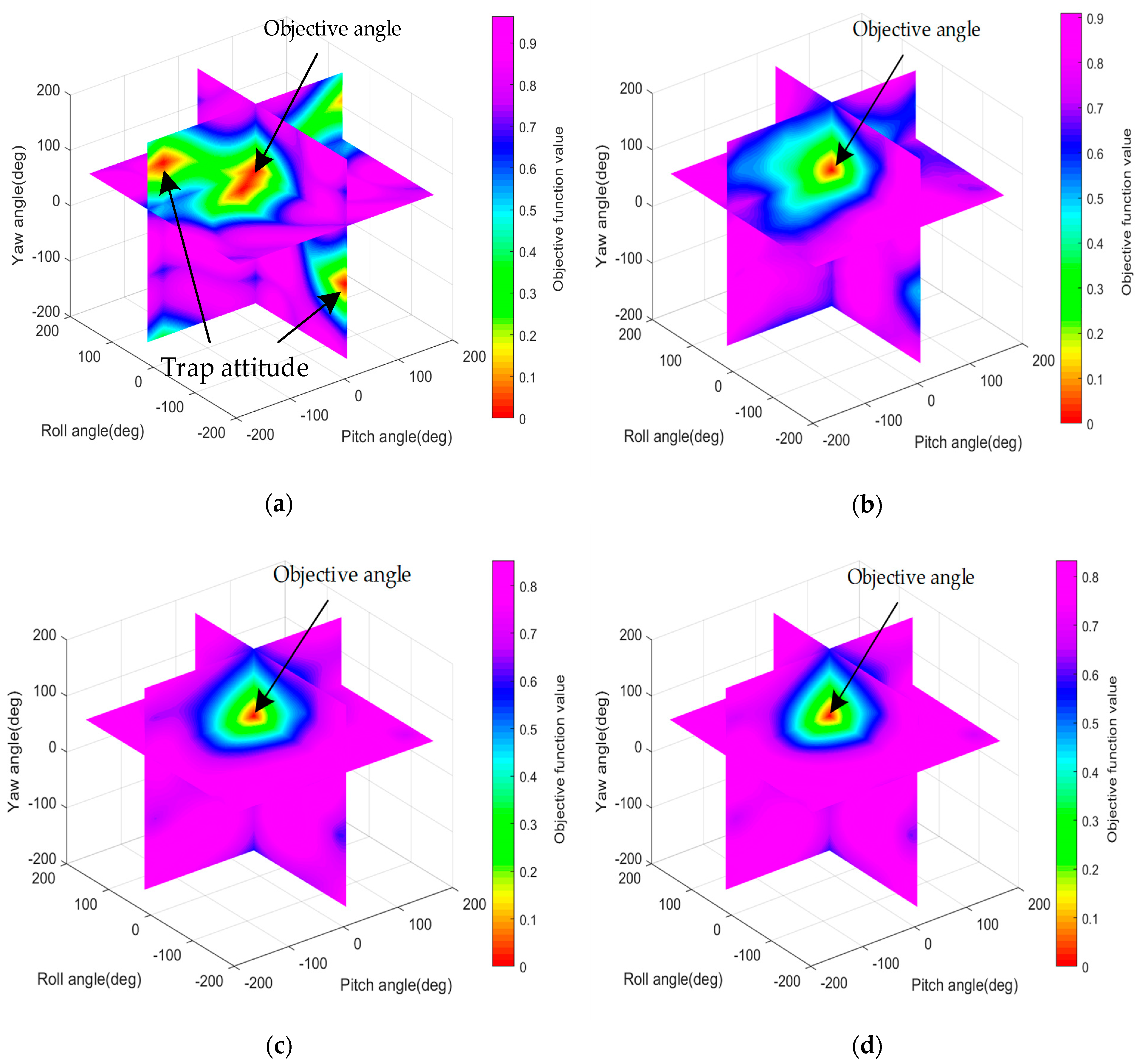
- The accuracy of double-vectors, which is an important prerequisite for the accurate attitude estimation, is improved by MDCM. The affect from the bias of inertial sensor is greatly reduced, so the double-vectors can be accurately constructed by this method on the low-cost navigation systems.
- The proposed optimal method based on gradient descent is more flexible. And it can meet various needs by adjusting the size of mini-batch in practical use. This method is very simple and easy to implement. This method does not involve any multi-dimensional matrix operations in the whole optimal estimation process. So it will consume fewer computing resources than the traditional methods and it is very friendly to low-performance processors.
- Our method has high accuracy and robustness. When the measurement contains bias of sensors and white noise, The proposed method has better performance than the traditional method represented by QUEST, which is proved by the results of simulations and experiments in this article.
Author Contributions
Funding
Conflicts of Interest
References
- Zhang, Y.; Yu, F.; Gao, W.; Wang, Y. An improved strapdown inertial navigation system initial alignment algorithm for unmanned vehicles. Sensors 2018, 18, 3297. [Google Scholar] [CrossRef]
- Chang, L.; Qin, F.; Jiang, S. Strapdown Inertial Navigation System Initial Alignment based on Modified Process Model. IEEE Sens. J. 2019. [Google Scholar] [CrossRef]
- Tian, X.; Chen, J.; Han, Y.; Shang, J.; Nan, L. Pedestrian navigation system using MEMS sensors for heading drift and altitude error correction. Sens. Rev. 2017, 37, 270–281. [Google Scholar] [CrossRef]
- Hu, H.; Zhang, J. Application of Hybrid Filtering Algorithm Based on Neural Network in INS/GPS Integrated Navigation System. In Proceedings of the 2018 IEEE 4th International Conference on Control Science and Systems Engineering (ICCSSE), Wuhan, China, 24–26 August 2018; pp. 317–321. [Google Scholar]
- Liu, Y.; Fan, X.; Lv, C.; Wu, J.; Li, L.; Ding, D. An innovative information fusion method with adaptive Kalman filter for integrated INS/GPS navigation of autonomous vehicles. Mech. Syst. Sig. Process. 2018, 100, 605–616. [Google Scholar] [CrossRef]
- Zhang, H.; Li, T.; Yin, L.; Liu, D.; Zhou, Y.; Zhang, J.; Pan, F. A Novel KGP Algorithm for Improving INS/GPS Integrated Navigation Positioning Accuracy. Sensors 2019, 19, 1623. [Google Scholar] [CrossRef] [PubMed]
- Zhang, Y. A Fusion Methodology to Bridge GPS Outages for INS/GPS Integrated Navigation System. IEEE Access 2019, 7, 61296–61306. [Google Scholar] [CrossRef]
- Kim, Y.; An, J.; Lee, J. Robust navigational system for a transporter using GPS/INS fusion. IEEE Trans. Ind. Electron. 2018, 65, 3346–3354. [Google Scholar] [CrossRef]
- Zhang, G.; Lu, C.; Li, Y. Research on Initial Alignment Method of SINS with Improved CKF. In Proceedings of the 2019 IEEE 3rd Information Technology, Networking, Electronic and Automation Control Conference (ITNEC), Sichuan, China, 15–17 March 2019; pp. 2315–2319. [Google Scholar]
- Li, J.; Xu, J.; Chang, L.; Feng, Z. An Improved Optimal Method For Initial Alignment. J. Navig. 2014, 67, 727–736. [Google Scholar] [CrossRef]
- Chang, L.; Li, J.; Chen, S. Initial Alignment by Attitude Estimation for Strapdown Inertial Navigation Systems. IEEE Trans. Instrum. Meas. 2014, 64, 784–794. [Google Scholar] [CrossRef]
- Li, J.; Li, Y.; Liuxs, B. Fast fine initial self-alignment of INS in erecting process on stationary base. J. Navig. 2018, 71, 697–710. [Google Scholar] [CrossRef]
- Lu, J.; Liang, S.; Yang, L. Analytic coarse alignment and calibration for inertial navigation system on swaying base assisted by star sensor. IET Sci. Meas. Technol. 2018, 12, 673–677. [Google Scholar] [CrossRef]
- Zhang, W.; Peng, G.; Yuan, B.; Wang, P.; Huo, Z.; Yang, Z. Improved Maximum Likelihood Filter Based on UD Decomposition Algorithm and its Application in Transfer Alignment. In Proceedings of the 2019 Chinese Control Conference (CCC), Guangzhou, China, 27–30 July 2019; pp. 4042–4048. [Google Scholar]
- Wei, X.; Huang, G.R.; Lu, H.; Peng, Z.Y.; Hao, S.Y.; Xu, M.Q. Marginal Reduced High-degree CKF and its Application in Nonlinear Rapid Transfer Alignment. In Proceedings of the 2018 International Conference on Computer Information Science and Application Technology, Daqing, China, 7–9 December 2018; p. 062030. [Google Scholar]
- Ding, Z.J.; Zhou, H.; Zhang, S.F.; Yang, H.B.; Cai, H. Initial Self-Alignment Method for Inertial Platform on a Stationary Base. J. Astronaut. 2017, 38, 612–620. [Google Scholar]
- Xu, Y.; Zhou, T. Research on In-Flight Alignment for Micro Inertial Navigation System Based on Changing Acceleration using Exponential Function. Micromachines 2019, 10, 24. [Google Scholar] [CrossRef] [PubMed]
- Wang, D.; Lv, H.; Jie, W. In-flight Initial Alignment for Small UAV MEMS-based Navigation via Adaptive Unscented Kalman Filtering approach. Aerosol Sci. Technol. 2017, 61, 73–84. [Google Scholar] [CrossRef]
- Wang, D.; Dong, Y.; Li, Q.; Wu, J.; Wen, Y. Estimation of small uav position and attitude with reliable in-flight initial alignment for MEMS inertial sensors. Metrol. Meas. Syst. 2018, 25, 603–616. [Google Scholar]
- Shuster, M.D. A survey of attitude representations. Navigation 1993, 8, 439–517. [Google Scholar]
- Pei, F.; Wei, X.; Liang, Q. A Fast Alignment Algorithm Based on Adaptive Quaternion Kalman Filter. In Proceedings of the 2017 9th International Conference on Intelligent Human-Machine Systems and Cybernetics (IHMSC), Hangzhou, China, 26–27 August 2017; pp. 312–316. [Google Scholar]
- Liu, J.; Zhao, T. In-flight alignment method of navigation system based on microelectromechanical systems sensor measurement. Int. J. Distrib. Sens. Netw. 2019, 15, 1550147719844929. [Google Scholar] [CrossRef]
- Wu, Y.; Pan, X. Velocity/Position Integration Formula Part II: Application to Strapdown Inertial Navigation Computation. IEEE Trans. Aerosp. Electron. Syst. 2013, 49, 1024–1034. [Google Scholar] [CrossRef]
- Shuster, M.D.; Oh, S.D. Three-axis attitude determination from vector observations. J. Guid. Control. 1981, 4, 70–77. [Google Scholar] [CrossRef]
- Markley, F.L. Attitude determination using vector observations and the singular value decomposition. J. Astronaut. Sci. 1988, 36, 245–258. [Google Scholar]
- Mortari, D. Euler-q Algorithm for Attitude Determination from Vector Observations. J. Guid. Control Dyn. 1998, 21, 328–334. [Google Scholar] [CrossRef]
- Wu, M.; Wu, Y.; Hu, X.; Hu, D. Optimization-based alignment for inertial navigation systems: Theory and algorithm. Aerosp. Sci. Technol. 2011, 15, 1–17. [Google Scholar] [CrossRef]
- Chang, L.; Li, J.; Li, K. Optimization-based alignment for strapdown inertial navigation system: Comparison and extension. IEEE Trans. Aerosp. Electron. Syst. 2016, 52, 1697–1713. [Google Scholar] [CrossRef]
- Xu, X. (Xiang Xu); Xu, X. (Xiaosu Xu); Zhang, T.; Wang, Z. In-Motion Filter-QUEST Alignment for Strapdown Inertial Navigation Systems. IEEE Trans. Instrum. Meas. 2018, 67, 1979–1993. [Google Scholar] [CrossRef]
- Wu, Y.; Pan, X. Velocity/Position Integration Formula Part I: Application to In-Flight Coarse Alignment. IEEE Trans. Aerosp. Electron. Syst. 2013, 49, 1006–1023. [Google Scholar] [CrossRef]
- Xu, X.; Xu, D.; Zhang, T.; Zhao, H. In-Motion Coarse Alignment Method for SINS/GPS Using Position Loci. IEEE Sens. J. 2019, 19, 3930–3938. [Google Scholar] [CrossRef]
- Wahba, G. A least squares estimate of satellite attitude. SIAM Rev. 1965, 7, 409. [Google Scholar] [CrossRef]
- Lerner, G.M. Three-axis attitude determination. In Spacecraft Attitude Determination and Control; Kluwer Academic: Dordrecht, The Netherlands, 1978. [Google Scholar]
- Keat, J. Analysis of Least-Squares Attitude Determination Routine DOAOP; Technical Report TM-77/6034; Computer Sciences Corporation Report CSC: Tysons, WV, USA, February 1977. [Google Scholar]
- Shuster, M. Approximate algorithms for fast optimal attitude computation. In Proceedings of the Guidance and Control Conference, Key Biscayne, FL, USA, 20–22 August 1973; p. 1249. [Google Scholar]
- Savage, P.G. Strapdown inertial navigation integration algorithm design part 1: Attitude algorithms. J. Guid. Control Dyn. 1998, 21, 19–28. [Google Scholar] [CrossRef]
- Xu, Y. Research on several key techniques of MINS/GNSS integrated navigation system in the guided projectiles. Ph.D. Thesis, Nanjing University of Science & Technology, Nanjing, China, 2016. [Google Scholar]
- Bao, J.; Qiao, X.; Li, D. Double-vector attitude determination algorithm improving coarse alignment accuracy of strapdown inertial navigation system for sea cucumber fishing device. Trans. Chin. Soc. Agric. Eng. 2017, 33, 286–292. [Google Scholar]
- Liu, M.; Gao, Y.; Li, G.; Guang, X.; Li, S. An improved alignment method for the Strapdown Inertial Navigation System (SINS). Sensors 2016, 16, 621. [Google Scholar] [CrossRef]
- Chang, L.; Zha, F.; Qin, F. Indirect Kalman Filtering Based Attitude Estimation for Low-Cost Attitude and Heading Reference Systems. IEEE/ASME Trans. Mechatron. 2017, 22, 1850–1858. [Google Scholar] [CrossRef]
- Ruder, S. An overview of gradient descent optimization algorithms. arXiv 2016, arXiv:1609.04747. [Google Scholar]


| Method | Errors(deg) | Alignment Time(s) | ||
|---|---|---|---|---|
| Pitch | Roll | Yaw | ||
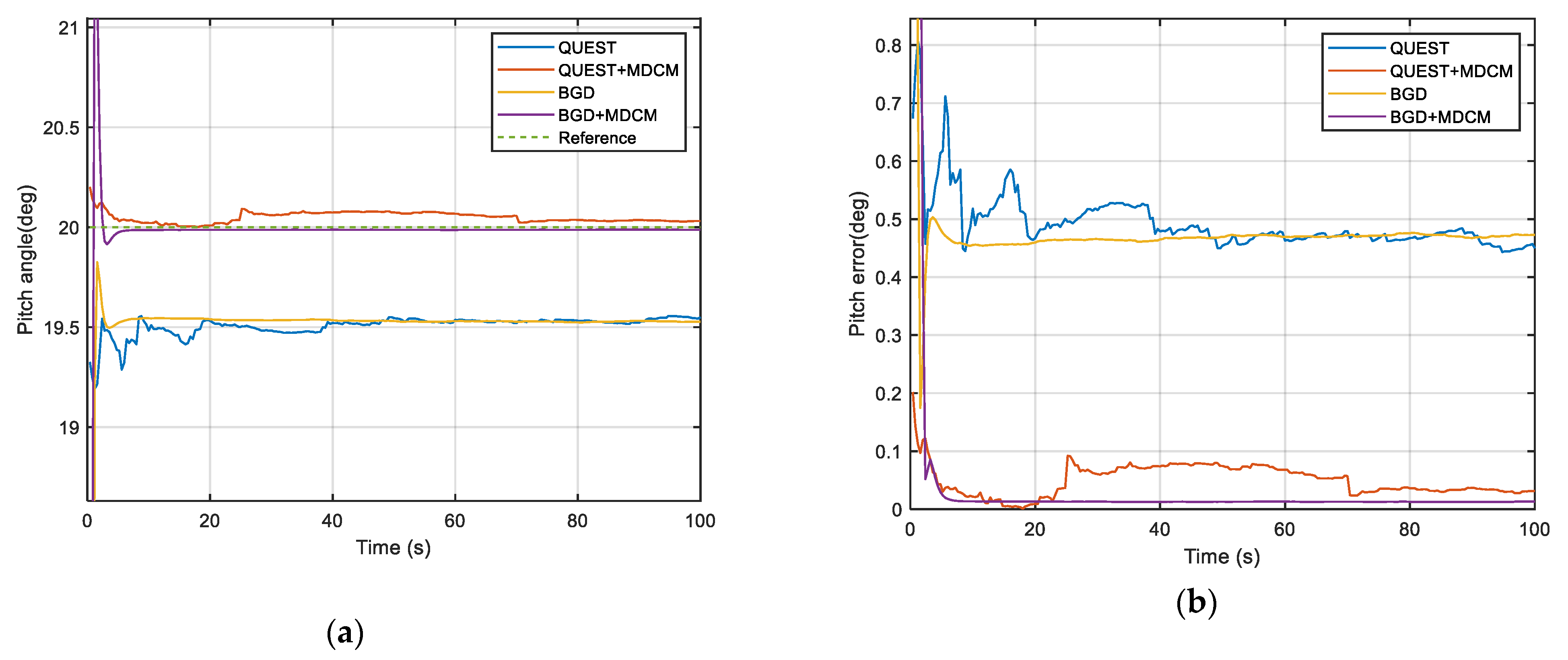
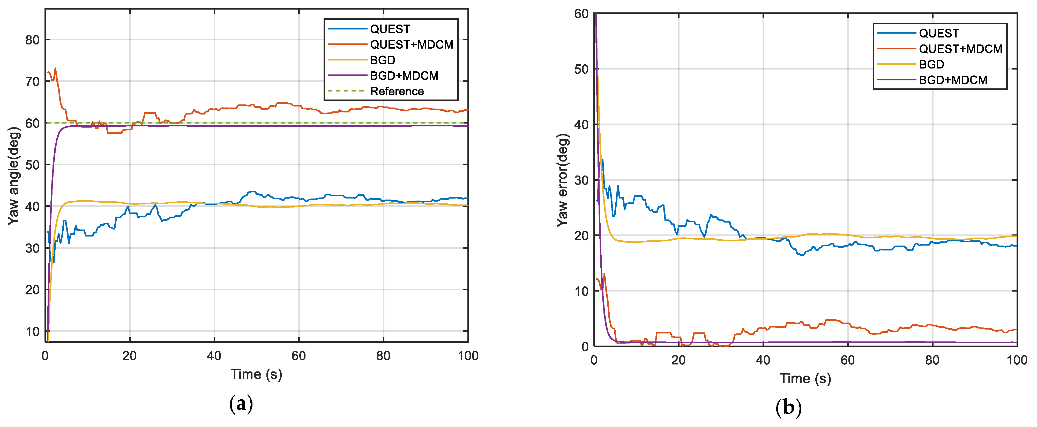
| QUEST | 0.493 | 0.824 | 20.34 | 39.20 |
| QUEST+MDCM | 0.050 | 0.055 | 2.95 | 37.85 |
| BGD | 0.462 | 1.17 | 20.01 | 8.08 |
| BGD+MDCM | 0.013 | 0.040 | 0.705 | 7.60 |
| Method | Errors(Degree) | Each Update Time 1 (ms) | Convergence Time 1 (ms) | ||
|---|---|---|---|---|---|
| Pitch | Roll | Yaw | |||
| SGD | 0.138 | 0.553 | 2.848 | 0.08 | 3.9 |
| MBGD(mini-batch = 10) | 0.032 | 0.155 | 2.352 | 0.13 | 5.8 |
| MBGD(mini-batch = 60) | 0.025 | 0.038 | 1.756 | 0.27 | 12.7 |
| BGD | 0.014 | 0.015 | 1.334 | 2.05 | 88.3 |
| Method | Errors(Degree) | Alignment Time(s) | ||
|---|---|---|---|---|
| Pitch | Roll | Yaw | ||
| QUEST | 0.037 | 0.022 | 2.69 | 38.79 |
| MBGD(mini-batch = 60) | 0.056 | 0.025 | 1.47 | 7.36 |
| BGD | 0.003 | 0.021 | 1.41 | 6.08 |
© 2020 by the authors. Licensee MDPI, Basel, Switzerland. This article is an open access article distributed under the terms and conditions of the Creative Commons Attribution (CC BY) license (http://creativecommons.org/licenses/by/4.0/).
Share and Cite
Lu, Z.; Li, J.; Zhang, X.; Feng, K.; Wei, X.; Zhang, D.; Mi, J.; Liu, Y. A New In-Flight Alignment Method with an Application to the Low-Cost SINS/GPS Integrated Navigation System. Sensors 2020, 20, 512. https://doi.org/10.3390/s20020512
Lu Z, Li J, Zhang X, Feng K, Wei X, Zhang D, Mi J, Liu Y. A New In-Flight Alignment Method with an Application to the Low-Cost SINS/GPS Integrated Navigation System. Sensors. 2020; 20(2):512. https://doi.org/10.3390/s20020512
Chicago/Turabian StyleLu, Zhenglong, Jie Li, Xi Zhang, Kaiqiang Feng, Xiaokai Wei, Debiao Zhang, Jing Mi, and Yang Liu. 2020. "A New In-Flight Alignment Method with an Application to the Low-Cost SINS/GPS Integrated Navigation System" Sensors 20, no. 2: 512. https://doi.org/10.3390/s20020512
APA StyleLu, Z., Li, J., Zhang, X., Feng, K., Wei, X., Zhang, D., Mi, J., & Liu, Y. (2020). A New In-Flight Alignment Method with an Application to the Low-Cost SINS/GPS Integrated Navigation System. Sensors, 20(2), 512. https://doi.org/10.3390/s20020512