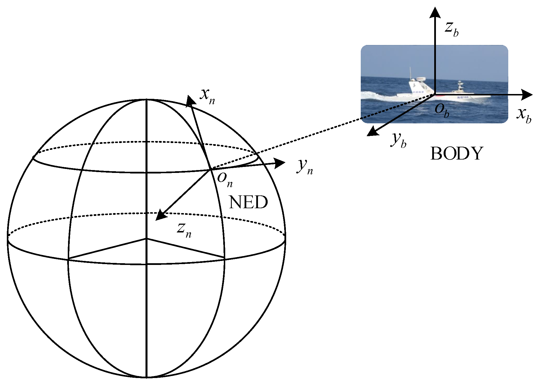
Since most ships do not have actuators in all degrees of freedom, the reduced-order model is often used. The 3 DOF horizontal plane model (surge, sway, yaw) is widely used in trajectory tracking control systems [
36] with the assumption of planar motion. A classic 3 DOF USV model, the accuracy of which is verified in [
37], is adopted in the following simulation work. The parameters of the vessel system are shown in
Table 1 and
Table 2. Additional details on the dynamic model are presented in
Appendix A, and the readers are referred to [
37] for further information.
5.1. IPT Results
According to the literature [
37], the maximum speed
of the USV is 18 kn. By using empirically determined values, the minimum turning radius, minimum speed and desired turning velocity are set as
m,
kn and
kn. In the cost function,
,
and
emphasize the turning radius, turning speed and path deviation, respectively. Users can tune the parameters accordingly to specific task demands. The weights of the cost function in this paper are chosen as
to emphasize on decreasing path deviations at turning corners rather than the needs to obtain small turning radius and high turning speed. The initial step size and step-size adjustment coefficient are set to
. The optimization process is terminated when the updated value of the path parameter is smaller than the user-specified positive value
.
To verify the convergence of the algorithm, three different groups of the path parameters
m,
,
, and
, are chosen as the initial values for the IPT simulations. To compare the performance of the TPA-IPT method proposed in this study with the fixed step-size version in [
28], simulations using both methods are conducted for each group, and the results are shown in
Figure 9 and
Table 3.
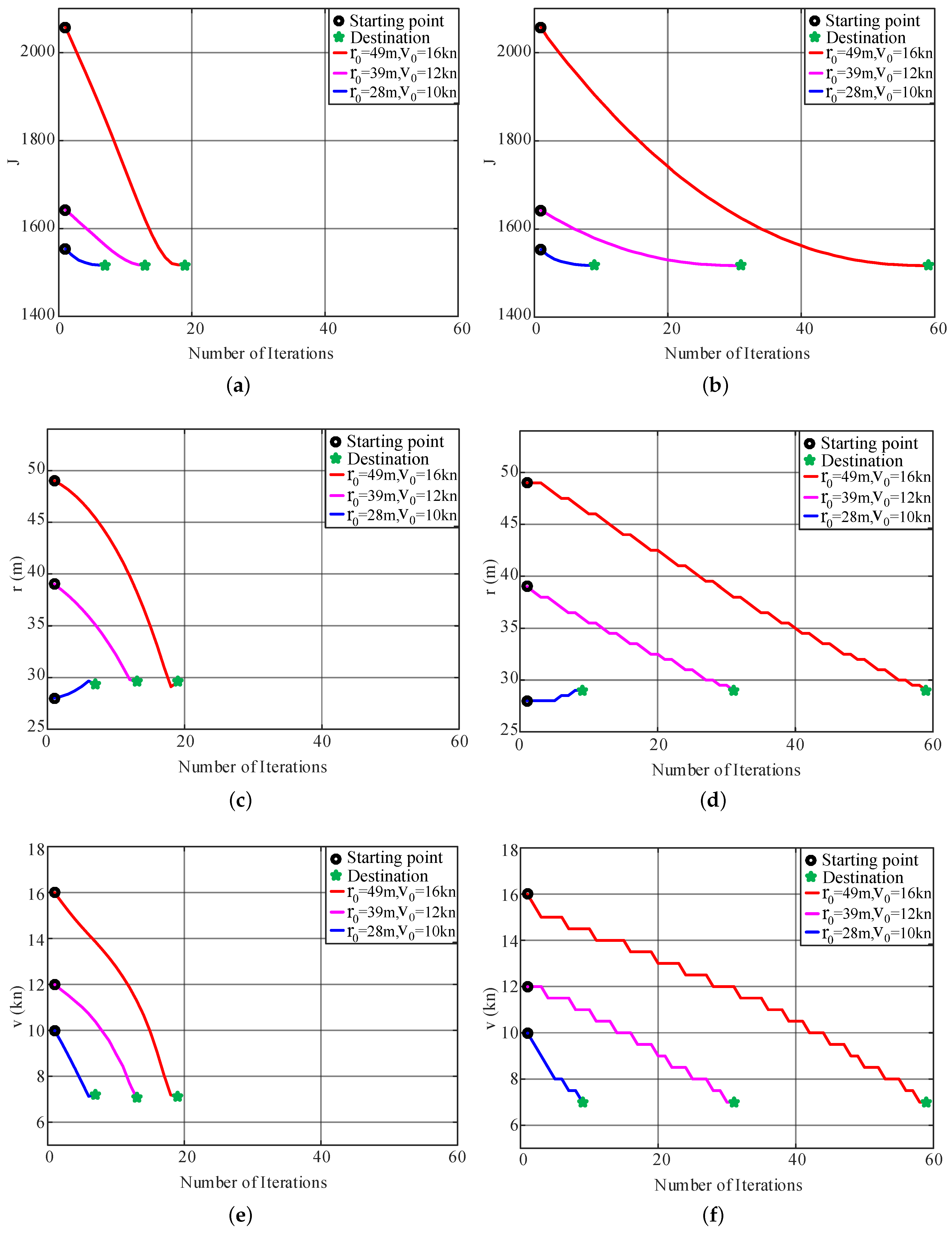
Figure 9a,c,e show the convergence of the cost function value and the two path parameters for each initial value set using TPA-IPT, and
Figure 9b,d,f are their counterparts for the fixed step IPT. It is observed that both algorithms can achieve a similar minimum point with small variance (
Table 3) regardless of how the initial value changes. However, the convergence speed of the TPA-IPT is much faster than that of the fixed step IPT.
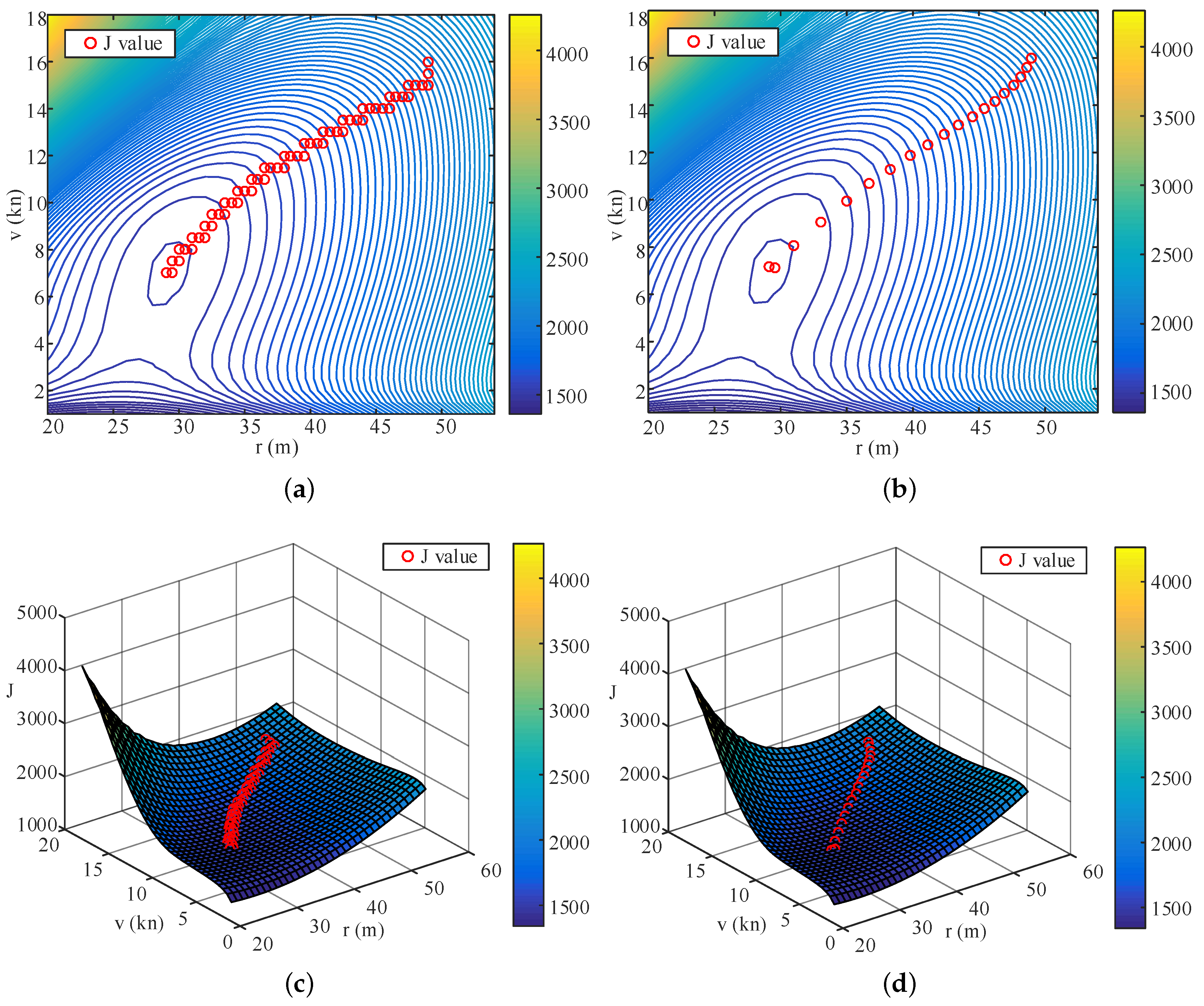
To perform a better comparison, the descent processes of the cost function value are drawn in
Figure 10 for the first group of the initial value by using both a contour graph and in a 3D cost function surface. The sharp slope of the function indicates that TPA-IPT speeds up and arrives at the minimum point with only 19 iterations, which is approximately one third of the number of iterations needed using fixed step IPT. For each iteration, TPA-IPT needs 2 more trials to adjust the step length. Therefore, the total number of trials needed by TPA-IPT is 114, which is less than half of the trial numbers for the fixed step strategy. This difference helps decrease the working load of the IPT tests when it is applied in real vessel tests.
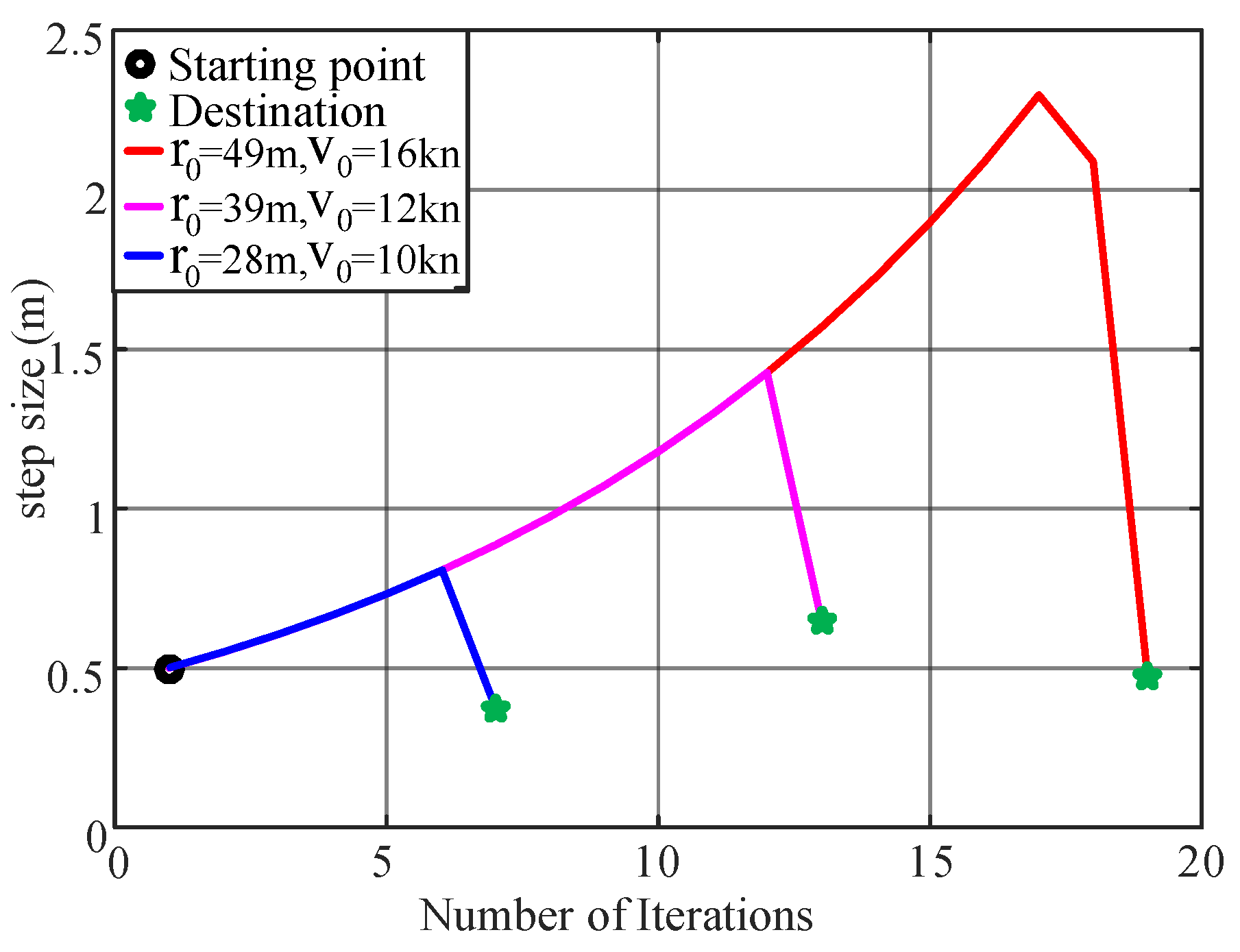
A similar result is obtained for other initial value setups. The variance of the step length using TPA-IPT is shown in
Figure 11, and a drop in the step size at the last several iterations is observed. This result is very reasonable considering the need for the fine tuning of the parameters when they are close to the minimum point.
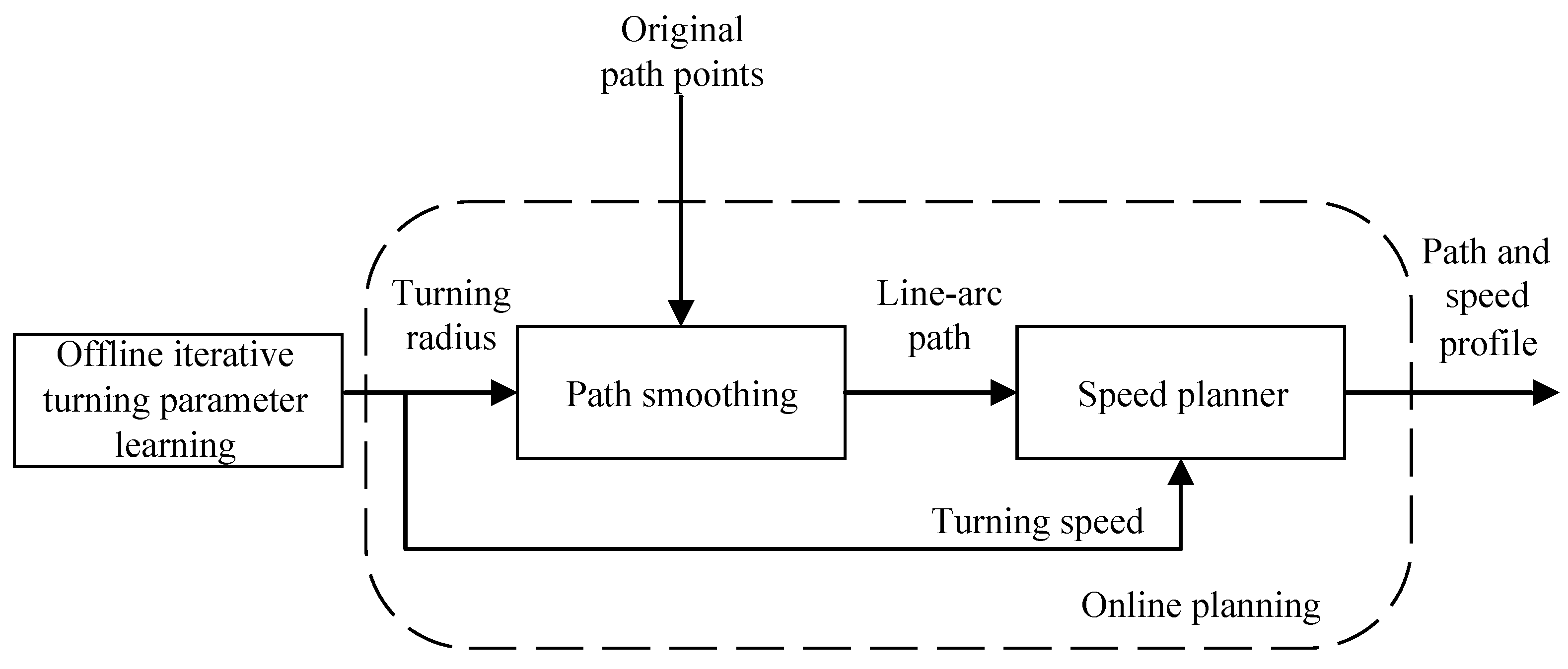
5.2. Path-Smoothing and Speed-Planning Simulations
Section 5.1 shows three sets of the initial path parameter values that are tested using the TPA-IPT method; these values provide close to optimal solutions for the turning radius and turning speed. The optimized tuning parameters
m,
kn will be used in the following work on the path-smoothing and speed profile-planning. To verify the effect of the path-smoothing and speed-planning algorithm, various turning conditions are designed. Four tested scenes, including a path with a large turning angle, a path with a small turning angle, a path for water sampling, and a path for bathymetric measurement, are designed to verify the performance of the proposed algorithm in this paper. The code was run on a computer with an Intel i5 2.30 GHz processor and 4.00 GB of RAM. To verify the real-time performance of the proposed algorithms, each test scene was run 10 times. As shown in
Table 4, the average time used for the path and speed profile calculation in the four test scenes are
s/km,
s/km,
s/km and
s/km respectively. In addition, the path-following performances are listed in
Table 5 with a comparison between the original and optimized path and speed profiles. As expected, the path-following accuracy and the drive safety are considerably improved when the method described in this study is used. The details on the results will be further discussed for individual cases in the following paragraphs.
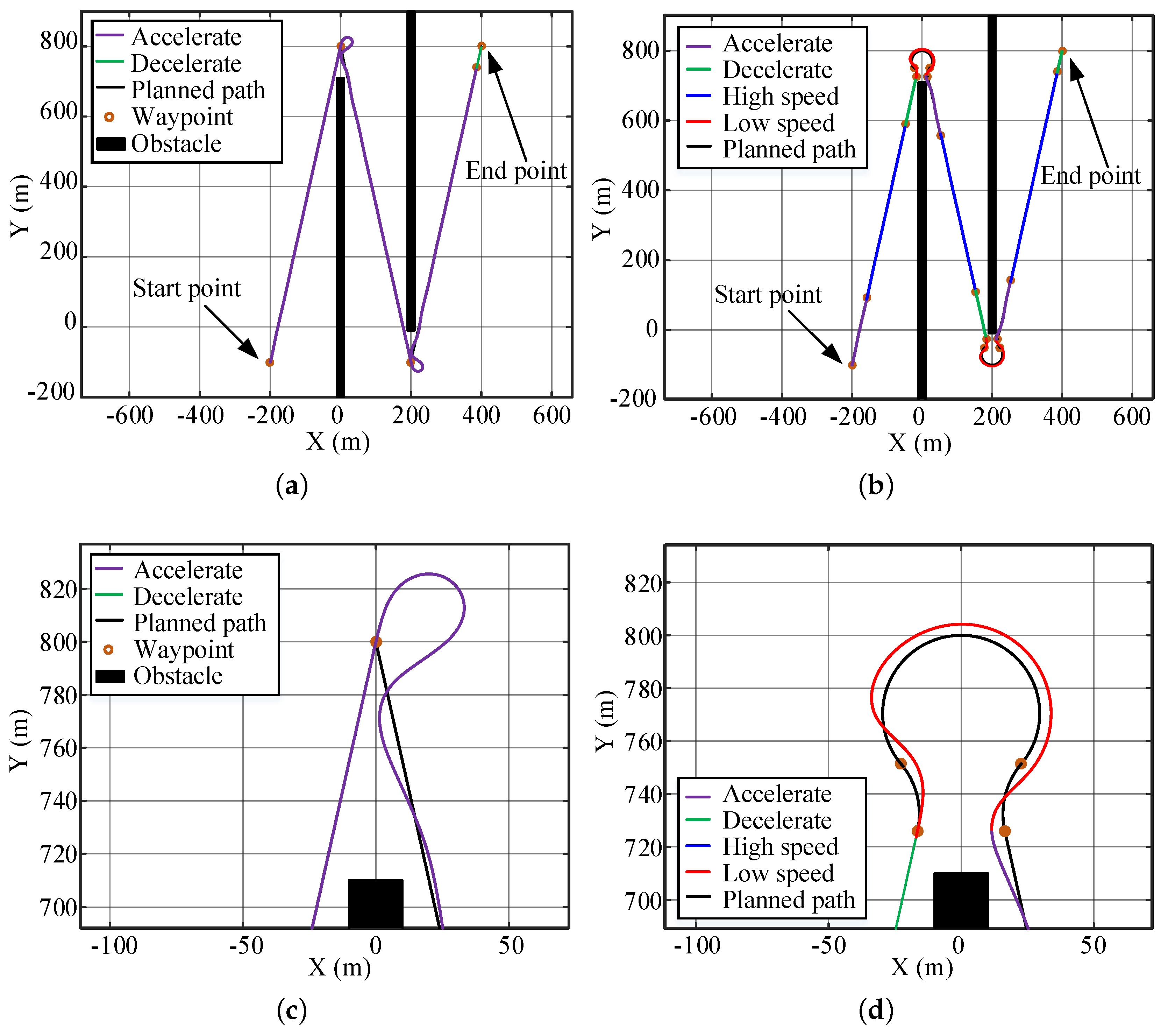
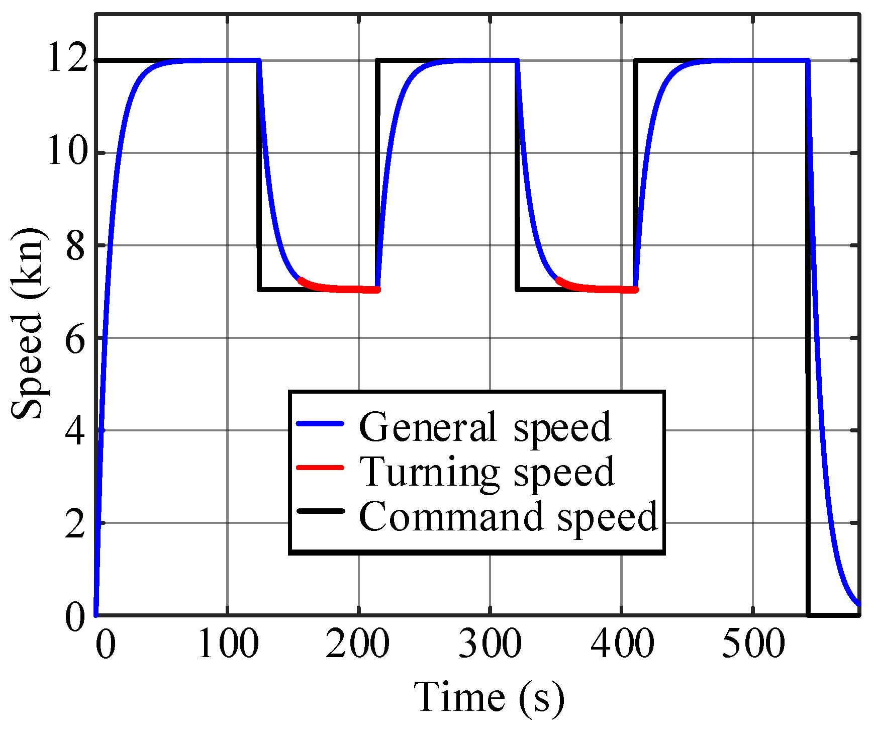
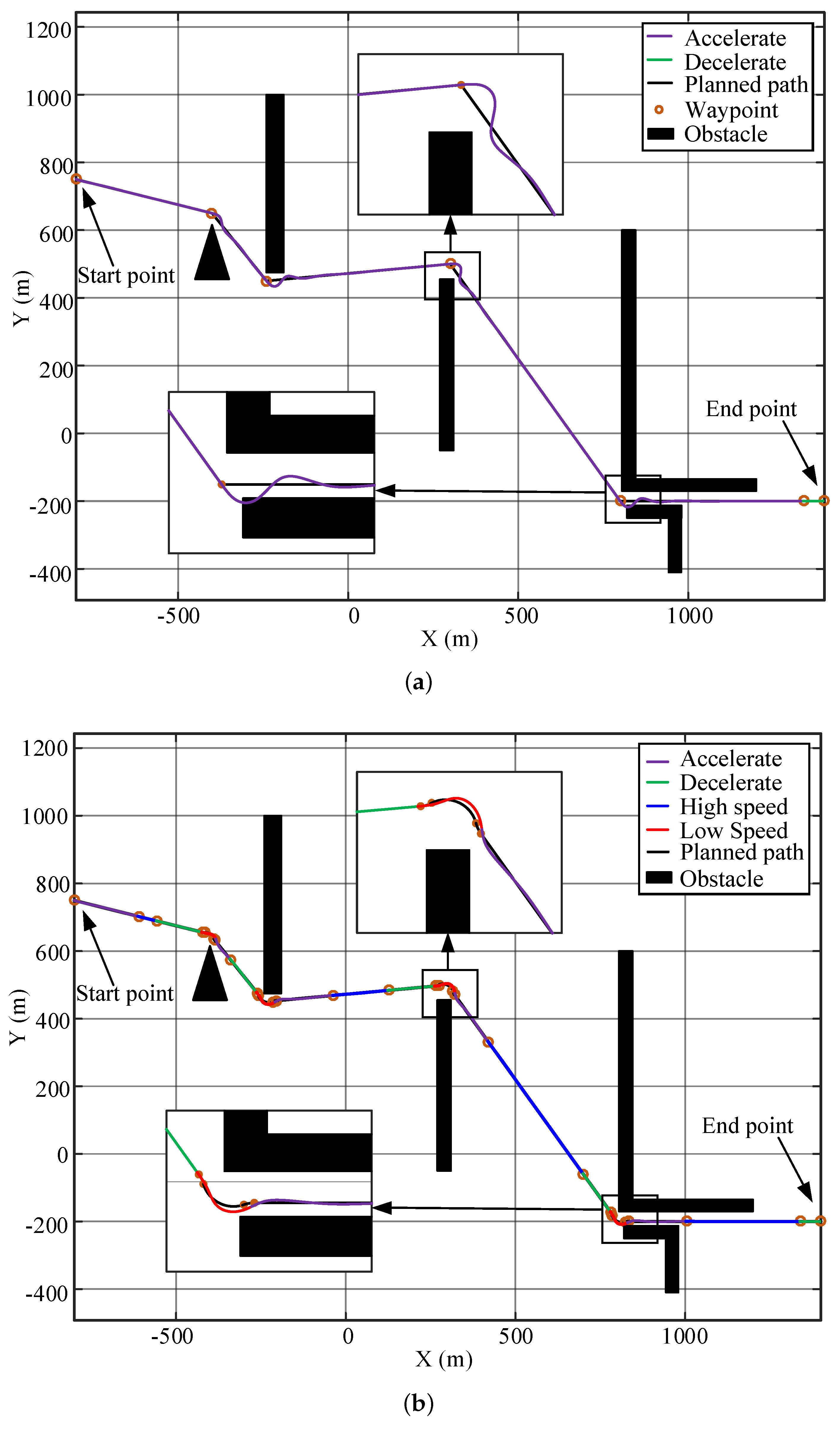
Figure 12 shows the simulation results for the large-angle turning scene. Black curves are the planned path, blue curves are the high-speed USV trajectories, red curves are the low-speed trajectories, the purple curve is the acceleration trajectory, and the green curve is the deceleration trajectory. The corresponding speed change for
Figure 12b,d are shown in
Figure 13. When the USV makes a large-angle turn at a speed of 12 kn, due to the limitation of dynamics, a large tracking error will be produced; this error will oscillate when returning to track the straight line, as shown in
Figure 12a,c. The maximum path error is
m, as shown in
Table 5. After applying the path-smoothing and speed-planning work proposed in this paper, it was found that the USV slows down near the turning corner and follows the curve at a speed of 7.05 kn. This algorithm agrees with the dynamics of USVs; therefore, the tracking error is small, and the oscillation is considerably reduced, as show in
Figure 12b,d. The maximum path error is
m, and the error value is insensitive to the path conditions. The maximum path error is reduced by
, and the driving of the USV is considerably stabilized with a small increase (
) in the travelling time.
For tasks with less demands on small path deviation and turning safety but more on small travelling time, the weight factors in (
1) should be readjust to have large
and small
. In this case, the resulted turning radius would be small, and the turning speed would be large using the IPT method. However, the authors do not recommend high-speed turning considering the risk of capsizing.
When the USV turns at small angles, the path-following performances of the USV without and with using the method described in this paper are compared. The influence of its dynamic constraints will decrease, as shown in
Figure 14a. Therefore, the maximum path deviation is originally
m, which is smaller than that for the large-angle case. By applying the path-smoothing and speed-planning algorithm, the maximum path deviation is decreased to
m, as shown in
Figure 14b. The displacement of the optimized path is
less than that of the original path, and the time used is
more than that of the original path. With a slight sacrifice of travelling speed, the method described in this paper shortens the travelling distance and, more importantly, considerably decreases the path-following error.
The decreased path deviation sometimes is vital for driving safety. As shown in
Figure 14a, the USV crashed onto an obstacle using the original path and speed profiles when it is turning into a narrow passage. The optimized path and speed design largely decreased the path deviation, and the USV successfully passed through the cluttered area, as shown in
Figure 14b.
Various situations for speed profile-planning are also designed to verify the algorithm in
Section 4. As shown in
Figure 14, the line segment between the triangular obstacle and the rectangular obstacle is too short to achieve full acceleration, which corresponds to the condition 2 in
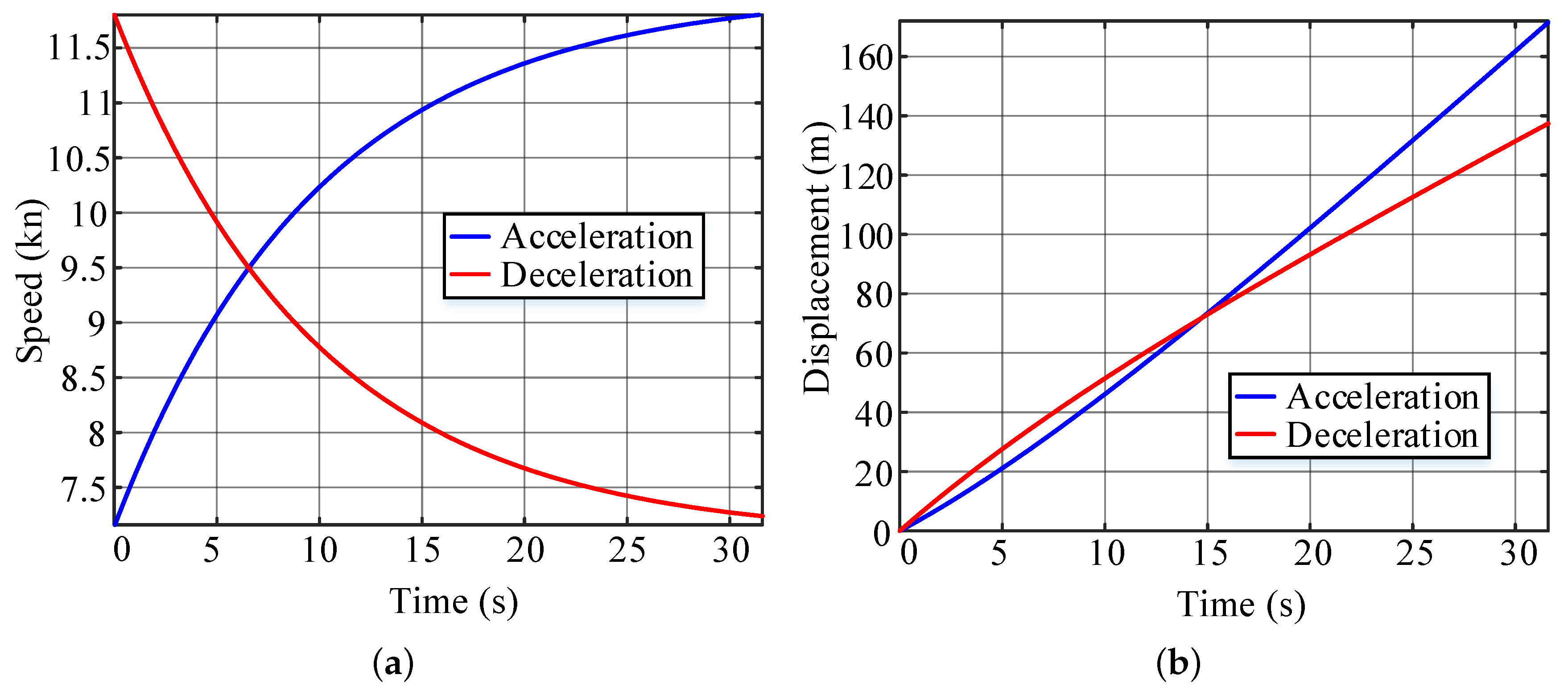
Section 4 for the speed profile-planning. With the acceleration and deceleration tests in
Figure 15a, the corresponding displacement curves are calculated and shown in
Figure 15b. Thus,
m,
m,
m. The length of the second line segment in
Figure 14 m
m. Thus, (
14) is used to plan the speed profile for the segment. The acceleration and deceleration distances in the straight-line segment can be obtained as
m,
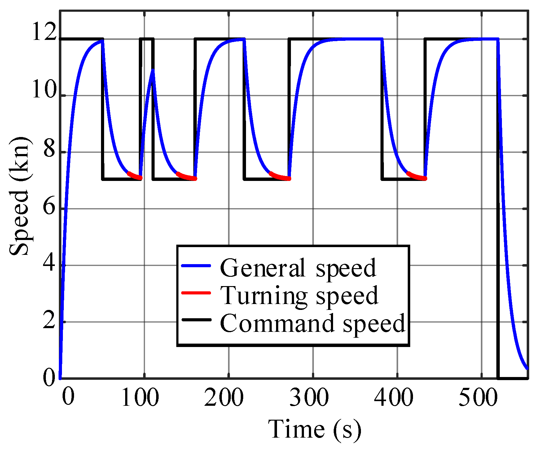
m. As shown in
Figure 16, the USV can reduce the speed to the optimal value before turning at the next corner.
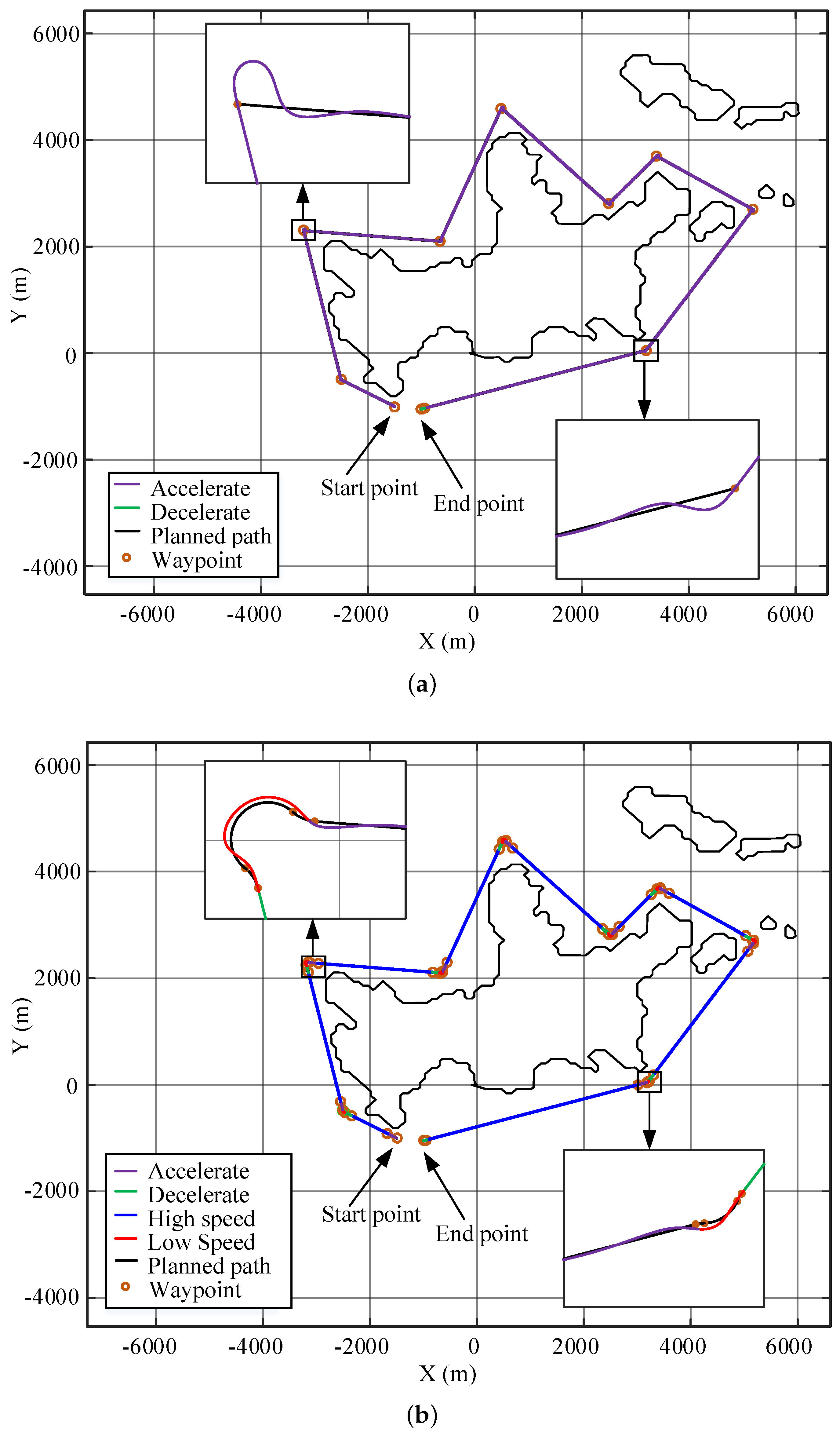
A similar result is obtained for the water sampling task around an island. A map of Mount Putuo, which is one of the 1390 islands in Zhoushan Archipelago, China, is drawn in
Figure 17. The sampling points scatter around the island and the USV needs to visit these points accurately to retrieve the water samples.
During the mission, the USV encountered two small-angle turns and six large-angle turns. As shown in
Figure 17a, the maximum path error at the corners by the original path and speed setup is
m, so the USV largely deviates from the desired sampling locations. By smoothing the path and planning the speed, the maximum tracking error can be reduced to
m, as shown in
Figure 17b. The motion stability of the USV is considerably improved, and the water samples are retrieved close to the desired locations.
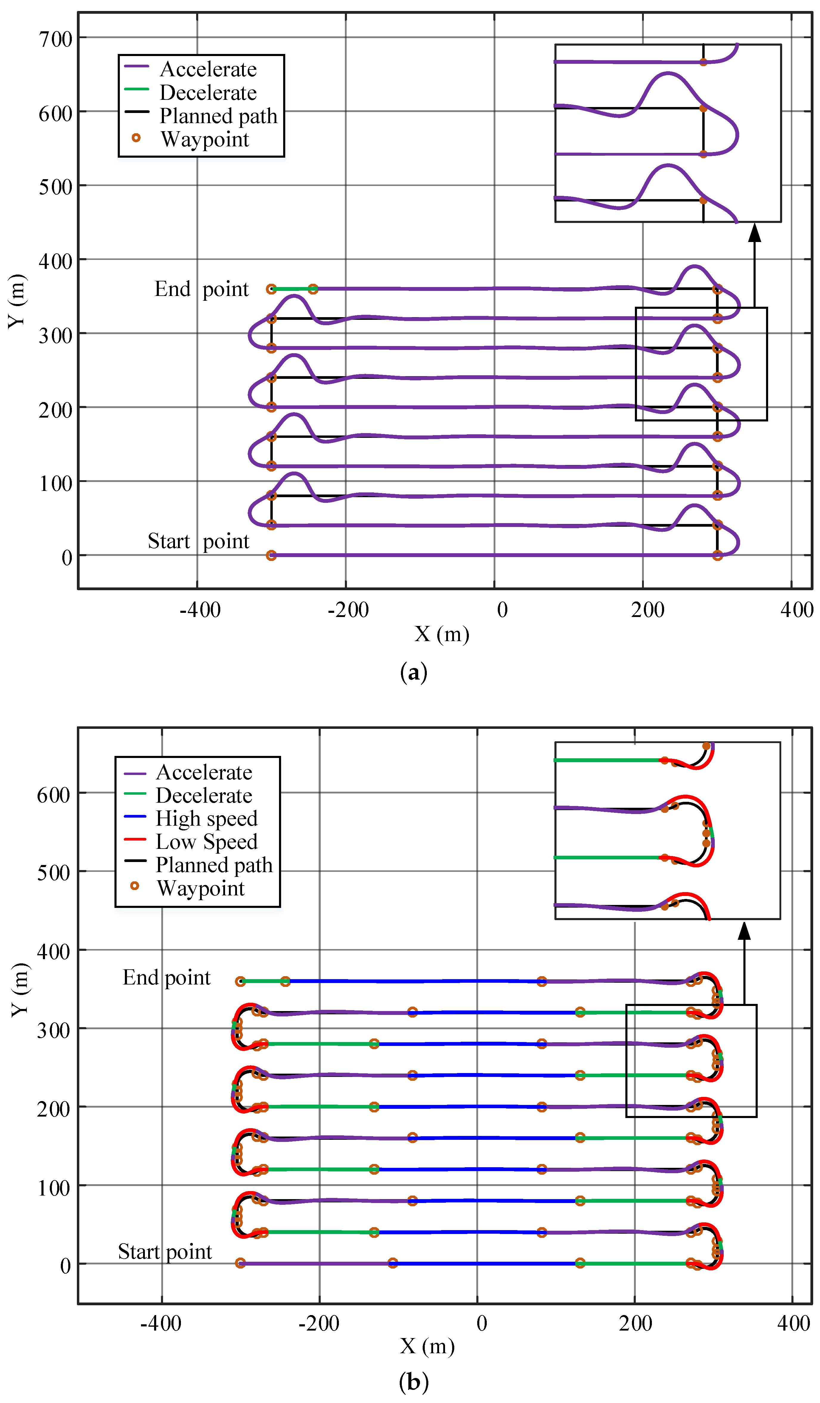
The bathymetric measurement is another example to show the benefits of the IPT method. As shown in
Figure 18, the USV needs to traverse an area to obtain the water depth data following a pre-defined path. This task requires the USV to have higher path-following accuracy and lower cruise speed [
2]. The new weights of the cost function and the minimum turning radius in the IPT algorithm are reset as
and
m. The remaining parameters remain unchanged. The original parameters
m,
kn were optimized by IPT to be
m,
kn. According to the line spacing in Reference [
38] and the property of the USV model, the line spacing is selected as 40 m.
As shown in
Figure 18, the maximum path deviation generated by the USV using the original cruise speed is
m, which is larger than the line spacing and causes intersections between the paths at the corners. This could leave some places uncovered at the corner areas. The path-following performance is greatly improved after path-smoothing and speed-planning, and its maximum path deviation is
m. In addition, the smooth actions at the corners can also help to reduce the measurement noises caused by highly dynamical turning behaviors of the USVs.


