1. Introduction
Urban sanitation systems involve sewer networks (SNs) and wastewater treatment plants (WWTPs). Integrated and joint management of these is mandatory to overcome issues arising from stormwater runoff episodes which, in short periods, overload the system in terms of pollutants and flowrates as well as those coming from the dry-weather daily variation of pollution load. Rainfall runoff collected and conveyed through combined sewers has an important influence on the efficiency of the entire treatment process [
1,
2,
3,
4]. Urban sanitation systems must comply with EU policies to halt the deterioration in the status of EU water bodies and the environment: Water Framework Directive (WFD, 2000/60/EC), Groundwater Directive (GWD, 2006/118/EC), Environmental Quality Standards Directive (EQS, 2008/105/EC), Directive 91/271/EEC or the Urban Wastewater Directive (UWWTD), Directive 2006/7/EC or the EU Bathing Water (Directive 2006/7/EC) and Marine Strategy Framework Directive (Directive 2008/56/EC). Continuous, real-time, reliable information about the pollutants in the input sewage is of great interest to improve and optimize the operation of the sanitation systems, to fulfill EU environmental policies and to reach European Green Deal targets [
5].
Developing sensors for the continuous monitoring of wastewater parameters is a major scientific and technical challenge due to the variability of wastewater characteristics as well as the extreme physical-chemical conditions the sensors are subjected to [
6,
7]. Optical techniques including UV–Vis spectroscopy and near-infrared spectroscopy NIR have been used to reliably characterize solids, organic matter and nitrates in wastewater for over a decade [
8,
9,
10,
11,
12,
13,
14,
15,
16,
17,
18,
19,
20,
21,
22,
23,
24,
25]. UV–Vis refers to the interaction between samples and radiation in the 200–780-nm wavelength range at single or multiple wavelengths to estimate a number of parameters [
19]. It is fast, non-destructive and environment-friendly since it does not require chemicals to be added. It is coupled with multivariate data analysis such as partial least squares (PLS) regression to generate a regression model based on spectral data to estimate the water quality parameters [
8,
26,
27,
28]. Several studies have shown good agreement in online continuous monitoring of chemical organic demand (COD) using UV–Vis spectroscopy [
8,
11,
16,
17,
18,
20,
22,
23,
24,
25]. Total suspended solids (TSS) has also been predicted through UV–Vis and NIR [
11,
17,
18,
22,
23,
24]. Nitrates (NO
3−N) achieved results with UV–Vis with an error of ~25% and correlation coefficients of 0.87 [
24]. Other works have presented the second derivative UV–Vis spectroscopy absorption spectrum for NO
3−N calibration [
10]. There are continuous sensors and analyzers capable of operating online with UV spectrophotometry that can be used to monitor nitrate and nitrite concentration in water samples [
14,
22]. Promising and long-term measurements have been developed in several cities, namely Linz [
21], Graz, Ecully and Vienna [
23], addressing online UV–VIS sensors for long-term sewer monitoring.
Statistical techniques have become necessary tools to establish correlations between optical sensors signals and the continuous monitoring of wastewater quality. Linear regression (LR) and other machine learning techniques such as support vector machine (SVM), evolutionary algorithm method (EVO) and artificial neural networks (ANNs) have been used for the mathematical treatment of spectral absorbance patterns to estimate five-day biochemical oxygen demand (BOD
5) and chemical oxygen demand (COD) values of wastewater samples [
11,
12,
13,
17,
19,
25]. From the absorbance response curves measured in an extensive range of wavelengths, specific measured values are used and combined through statistical techniques to generate a relation between pollutant concentration and absorbance or transmittance. The slope transmittance calculation and other mathematical operations such as the second derivative are also used for the estimation of biochemical loads [
10,
15,
27].
Deploying spectroscopic-based sensors throughout the sewerage system to monitor the pollution load in real time requires an enormous amount of equipment that must therefore meet the requirement of being cost-effective. The literature already describes the availability of compact and low-cost UV–Vis spectrophotometers to monitor WWTP processes [
29,
30,
31,
32,
33,
34,
35,
36,
37,
38,
39,
40]. In addition, the installation of storm water storage and sedimentation tanks is usually economically unacceptable, thus a monitoring system to optimize the management of the sewer network is the most cost-effective and, probably, the most ecological variant as well [
16]. Despite this scenario, the number of online studies remains relatively limited due to certain drawbacks such as the variability of sample composition and other matrix effects (particle size and moisture content) that complicate the absorbance response correlation [
19].
The present work shows a full-scale WWTP study for the estimation of chemical oxygen demand (COD), biological oxygen demand at five days (BOD5), total suspended solids (TSS), phosphorus (P), total nitrogen (TN) and nitrate nitrogen (NO
3−N) by means of site-specific multivariate linear regressions (MLR) and machine learning genetic algorithms (GA) from the absorbance and transmittance in the UV–near visible and visible 380–700 nm wavelength range. A campaign of around 1200 analytical determinations in the lab was carried out in the Cabezo Beaza WWTP (Region of Murcia, Spain), during the period from June 2019 to April 2020. The samples were collected from the Influent Wastewater (Raw water) and Effluent treated water of the WWTP. They consisted of six classes of contaminant analysis (COD, BOD5, TSS, P, TN and NO
3−N). Each class had a size of approximately 200 samples. About half of the samples corresponded to the input of the WWTP (raw water) and the rest to the output (treated water). The equipment used for the transmittance characterization in the UV–near visible and visible range is cost-effective, own developed and has been previously calibrated [
29]. This is an offline research study, considered as the first step to reaching a continuous and online monitoring system, at sanitation-system scale, which allows assisting in the control of the pollutants that reach the treatment plant, as well as contributing to the improvement of the treatment processes carried out.
The rest of the article is organized as follows:
Section 2shows all the materials and methods used for the development of the research work. It describes the characteristics of the experimental campaign carried out, indicating the conditions for data collection, the number of samples analyzed and the polluting parameters under study. It also includes a description of the equipment developed for the process of characterizing the samples, as well as the different calculation procedures used to obtain the models for estimating the pollutant load from the spectrophotometric data. In
Section 3, the characteristics of the analyzed water, both raw and treated, are described, as well as the different models for the estimation of the pollutant load obtained by the multivariable linear regression models, as well as the genetic algorithm. The results and comparisons of the models are also presented. Finally,
Section 4 discusses the considerations reached at the end of the research work.
2. Materials and Methods
2.1. Experimental Campaign
Samples were collected in the waterline of the Cabezo Beaza WWTP at two different sampling points, in the period June 2019 to April 2020:
Influent wastewater at the entrance of the WWTP: raw water
Treated water, at the exit of the secondary settler, prior to the third treatment: secondary wastewater
Responding to the requirements of the inspection sampling campaigns by the supervisory administration (Wastewater Administration of Murcia Region, ESAMUR), the samples were integrated, i.e., they were taken homogeneously during 24 h in a 5-L volume, by means of an accumulated sample of 200 mL/h. After this, they were collected around 7:00 AM daily and tested almost simultaneously. Once in the laboratory of the plant, the samples used in the present research were not pre-treated through any filtering process, with the intention of reproducing the conditions of automatic sampling for the continuous monitoring sensors. Tests at the WWTP lab were in correspondence with Standard Methods (SM) and International Organization for Standardization (ISO), as described in
Table 1. Standard methods were developed by members of the Standard Methods Committee (SMC) with the mutual publication of the American Public Health Association (APHA), American Water Works Association (AWWA) and the Water Environment Federation (WEF).
To develop the statistical models to estimate the pollutant load from the spectrophotometric data between 380 and 700 nm, it was necessary to obtain two datasets for each of the samples: the input data, based on the spectrophotometric analysis of the samples, and the analytical values of the pollutant load measured by the WWTP’s laboratory (output data).
2.2. Spectrophotometric Device
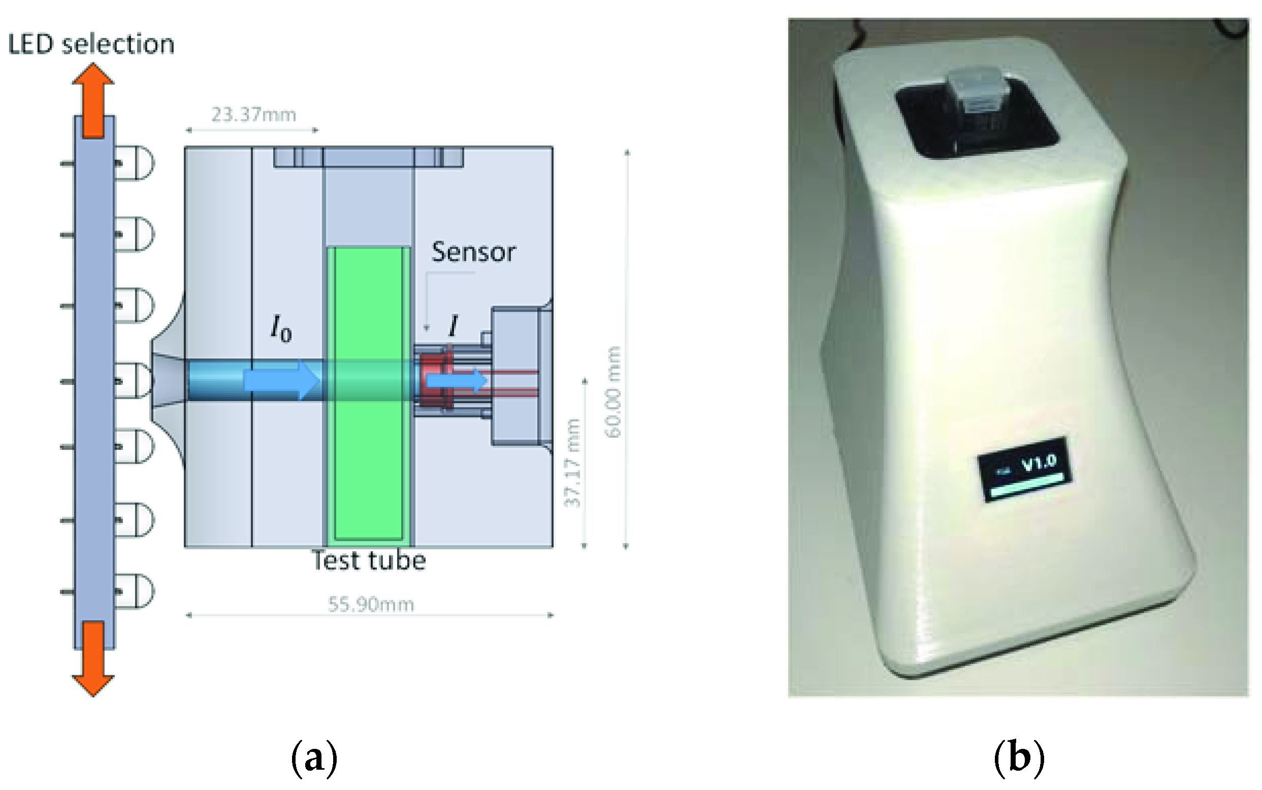
Figure 1 shows a schematic view of the spectrophotometry equipment based on LED technology (
Figure 1a) and an image of the equipment (
Figure 1b), which we developed to analyze the spectral response of wastewater samples. This device was previously calibrated with a commercial spectrophotometer in the UV–near visible and visible wavelength range 380–700 nm and the results were presented in previous research [
29]. This is a cost-effective piece of equipment which, to reduce its size and to improve its portability, uses no optical element such as lenses, diffraction matrix, or monochromators. The interior of the proposed assembly was constructed entirely in black thermoplastic PLA with a 3D printer, while the outer casing is made of white PLA, although the color of the casing does not affect the operation of the device.
From the results of the research conducted in [
29] on the use of LED technology, the device can model 81 wavelengths within 380–700 nm using only 33 limited-bandwidth LEDs. To select the working LED, the equipment has a motorized system consisting of a panel that slides vertically, which has all the light-emitting diodes, so that they can be aligned with the sample being analyzed.
The light from the LED passes through the sample via a 6-mm-diameter channel to the sensor [
30]. The sensor S1223, whose accuracy was previously studied, was chosen for the analysis of the samples [
29,
31]. The tests carried out revealed that the most accurate results were obtained when the sensor (
Figure 1a, right) was as close as possible to the sample without touching it, and the light source (
Figure 1a, left) [
32,
33,
34,
35,
36,
37,
38,
39,
40] was at a distance of about 23.77 mm with regard to the test tube. All samples were stored in standard 12 mm × 12 mm × 50 mm plastic test tubes of the SEOH brand [
41], designed for spectrophotometry purposes.
2.3. Regression Models
2.3.1. Multivariate Linear Regression
A multivariate linear regression (MLR) model is proposed where the entire evaluation of the transmittance and absorbance spectra within 380–700 nm is used. As input variables, both the transmittance and the absorbance values obtained by the 81 wavelengths supported by the developed equipment were used, giving rise to 162 variables.
To be able to validate the models calculated with data not used during their collection, the data were divided into two groups: training data (for the development of the models) and test data (for the validation of the models). These data were divided at random with proportions of 66% and 34%, respectively.
The MLR model was developed with the IBM SPSS Statistics software, using a model fitting based on partial least squares [
42]. A prior step to the calculation of any model is to determine the existence of outliers. A box and whiskers diagram was built to determine the existence of outliers and subsequently eliminate them. To make a multivariate model, the data must follow a normal distribution, i.e., that the P-value is greater than 0.1 (90% confidence interval) calculated with the Kolmogorov–Smirnov and Shapiro–Wilk tests. If it does not follow a normal distribution, the Box–Cox transformation [
43] should be carried out.
Once the data follow a normal distribution, SPSS tools are used to perform the analysis, selecting the “Stepwise” [
44] calculation option, which allows for more optimized calculation models. Therefore, the wavelengths (regressors) present in each of the MLR models were automatically selected by SPSS according to the following methodology.
The process starts by introducing the regressor whose P-value is highest within the range 0.05 and 0.1 (input and output criteria, respectively). In the following interaction, SPSS reintroduces the regressor with the highest p-value (within the range) and then reevaluates the model to check if any of the regressors introduced are no longer significant and/or there is multicollinearity in the model, i.e., that there are regressors correlated with each other in the model. This process is repeated with all possible combinations of regressors.
Once SPSS has calculated the models, those whose coefficient of determination R-square () is greater are selected and a check is made to ensure that the model does not include correlated variables, by checking that the Variance inflation factor is less than 7.
2.3.2. Genetic Algorithms
Another statistical technique used in the present work is the genetic algorithm. This was developed to calculate correlation models between the input variables (spectrophotometric data) and output variables (contaminating parameters) of water samples.
Within the category of genetic algorithm, a type of model known as “symbolic regression” was implemented, which is a type of regression analysis that seeks the space of mathematical expressions to find the model that best fits a certain dataset. The calculation model was developed in Python using the following libraries: TensorFlow [
45], NumPy [
46,
47] and gpLearn [
48]. Before processing the data, outliers were removed using Box and Whisker analysis for the response variable. Symbolic regression works through a system of “trees” composed of interconnected nodes. Each of these nodes can be composed of a variable (transmittance and absorbance values for each of the 81 wavelengths, i.e., 162 variables) or operators/functions (addition, subtraction, division, multiplication, trigonometric functions, etc.)
The process of finding a model that correlates the input variables with the output variables is based on an evolutionary process. As a starting point, we used both multivariate linear regression models calculated for the pollutant parameters as well as randomly initialized functions based on certain restrictions of length and type of operators. This evolutionary model has 100 generations, where 1000 different trees are generated in each generation, with a mutation rate of 15% by the subtree swapping method [
49,
50,
51,
52,
53,
54]. Each tree is generated starting with an addition node, from which a random number of nodes are derived, which can be constants, variables or operations. The nodes consisting of operations will have new descending nodes, which can once again be constants, variables or operations. The branching process of the tree continues until all the terminations are constant or variable or the total length and/or depth of the tree is exceeded. Each randomly generated tree is tested with the input data (absorbance/transmittance) in order to check how close the response variable (the pollutant load, e.g., COD) is to the values calculated by the WWTP. The trees closest to this result will be mutated (combined) to generate another 1000 trees, and the process is repeated until 100 generations are completed.
Each time the model calculation process is started, the GA takes the training data at random in the first iteration and based on that selection calculates the model. To guarantee the validity of the models presented, a cross-validation process was carried out, consisting of the repeated execution of the model generation process, in order to obtain different estimation models for each parameter. In all cases, the models presented a very similar level of accuracy, although their mathematical expressions (coefficients) were different. Therefore, in the present manuscript, only one of the multiple calculation models is shown, since all of them are equally valid.
It is important to point out that the data were subjected to the same process of detection and elimination of outliers described in
Section 2.3.1 for MLR before being analyzed.
The symbolic regression (genetic algorithm), is based on the development of a neural network, which must be trained and tested. As training data, we used 66% of the input data, taken at random, while the remaining data were used to test the validity of the calculated models, also taken at random.
This ratio was chosen according to the design criteria in [
55,
56], which recommend a ratio of 70%:30% when dividing the data. However, to achieve a more generalist model, that is, one that does not depend so much on the input data used, we decided to use the ratio 66%:34%.
The formulas generated by the algorithm can have a variable extension, include all types of operations, both arithmetic and trigonometric, exponential, or logarithmic functions, as well as more or fewer parameters.
2.3.3. Model Comparison
To be able to make a comparison between the two types of models (MLR and GA), several parameters were calculated: the Root-Mean-Square Deviation (RMSD) [
57] and the error index, Er, through Equations (1) and (2):
where
n is the number of samples; and
and
are the values of the polluting parameters (COD, BOD
5, TSS, P, TN and NO
3−N) obtained by the analytical methods used by the wastewater treatment plant and by the calculation models, respectively. It is necessary to point out that negative error value denote that the calculated models tend to provide lower than expected estimates, as opposed to positive values.
2.4. Data Platform
To enable the relations between the transmittance/absorbance data provided by the LED-Spectrophotometer and pollutant parameters measured by the wastewater treatment plants to be determined, all the information generated has been stored in a single website [
58], so that it can be easily downloaded in CSV format for further analysis.
Each of the stored samples contains information on the date and time of its analysis, identification of the equipment used to measure it, identification of the wastewater plant that carried out the analysis, and the spectrophotometric data and polluting parameters calculated by the treatment plants.
Figure A1 (
Appendix A) shows a view of the web platform for data storage.
2.5. Comparison with Commercial Equipment
Due to the difficulty of carrying out real-time analysis of wastewater quality, many researchers have developed analysis systems based on indirect measurements of the pollutant load, such as turbidity.
Systems such as those presented in [
59,
60] are able to carry out the analysis of turbidity of samples through the use of LED technology and low-cost photosensors. The equipment described in [
59] consists of a probe that allows the measurement of transmittance and lateral light scattering generated by a set of LEDs of different wavelengths, using two broad-spectrum photodiodes. This allows them to measure the degree of opacity of water samples with great precision, in addition to measuring other parameters such as chlorophyll, which is very useful for analyzing water quality.
Other equipment, such as those presented [
61,
62], go a step further and combine turbidity analysis with other sensors that allow measuring the amount of nitrates, dissolved oxygen, or conductivity of the samples, among others. These parameters are very useful when trying to know the water quality in a fast way and in real time.
This research work sought to develop a simpler system, where external sensors are not required to carry out an analysis of water quality, in order to obtain a smaller and cheaper equipment. To do this, unlike previous systems that make use of measurements of the turbidity of the samples, that is, one or a small number of wavelengths, the system presented in this research work determined, from a wider range of wavelengths (380–700 nm), the values of COD, BOD5, TSS, P, TN and NO3−N with a high precision and without the need to rely on external parameters such as conductivity or temperature.
In contrast to the previous systems, it is worth mentioning the s::can’s [
63] system. This system is capable of analyzing multiple parameters of contaminants from the spectral response of water samples taken in real time, in a similar way to the system presented in this research work. However, although this equipment is capable of generating a wider emission spectrum, it is based on xenon lamps. These lamps have high energy consumption and require the use of diffraction gratings to diffract the light beam before reaching the CCD sensor, which are responsible for its almost 500-mm length. This also increases the cost of the equipment and significantly increases its dimensions. The equipment developed in this research work is based on the use of LED diodes, where, as was verified in previous works [
29], the use of optical elements is not required to function.
3. Result and Discussion
3.1. Transmittance Characterization and Sampling Analysis
A wastewater plant carries out analyses at different points in its treatment process to check how the treatment process is working. At each of these points, the pollutant load changes, as do the biological matter and inorganic particles present in the water, which react at certain wavelengths. Spectrophotometric analysis can also be used to observe these variations at each point in a wastewater plant.
Spectrophotometry is based on the amount of light that passes through the samples at certain wavelengths, which depends on the physical-chemical characteristics of the samples.
In treated water, the concentrations of organic and inorganic matter are very low, which means that all the wavelengths of the visible spectrum can pass through more easily, giving rise to a more horizontal emission spectrum, without significant changes. It is this absence of variations in the spectral response that makes it difficult to find patterns that allow the pollutant load to be estimated from spectrophotometric data.
The tests carried out showed that the greater is the pollutant load, the easier it is to find correlations between transmittance/absorbance data and the pollutant concentration measured in the treatment plants.
Taking into account how transmittance data evolve with respect to the pollution concentration, it is essential to find the correlations between them.
Section 3.1.1 and
Section 3.1.2 show an example of the spectrophotometric response of the samples, together with their respective pollutant parameters, at each of the main analysis points in the wastewater treatment plant, in order to show how the pollutant load affects the transmittance and absorbance results.
3.1.1. Wastewater (Raw Water)
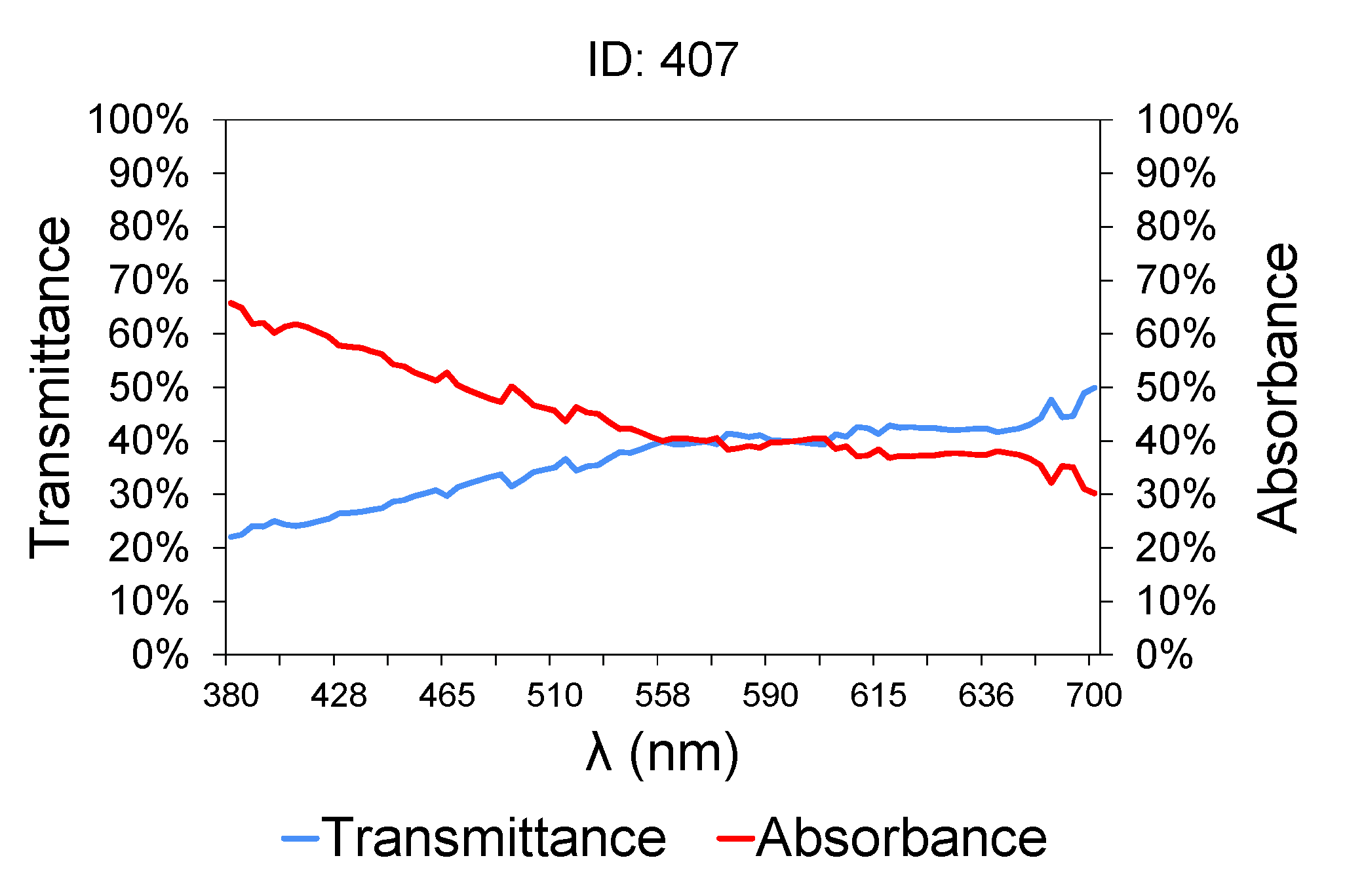
Figure 2 shows a sample of wastewater taken at the intake of the treatment plant (raw water).
Table 2 contains the characteristics of the sample shown in
Figure 2. The lower is the transmittance graph, the higher is the contaminant load of the samples, because of their higher turbidity [
64,
65]. Between 380 and 700 nm, the graph shows an upward slope, which is much steeper between 380 and 558 nm, and then tends to level out [
66]. The transmittance graph from 558 nm upwards is typically constant in all the samples, and the transmittance value did not exceed 50% in any case. Therefore, attention should be paid to the region between 380 and 558 nm. A small variation in the transmittance value at 380 nm between different samples involves a large variation in COD, BOD
5, TSS and TN values [
67,
68]. Others such as conductivity [
69] and PH [
70] bear no relation to variations in transmittance and absorbance.
This variation in slope is due to the greater sensitivity of organic matter to ultraviolet light. At low wavelengths in the UV near-visible range, close to 380 nm, organic matter absorbs more radiation and therefore less light is able to pass through the sample (lower transmittance). As the wavelengths are moved away from the ultraviolet/blue area, the organic matter absorbs less light and the change in transmittance is less significant.
3.1.2. Treated Water
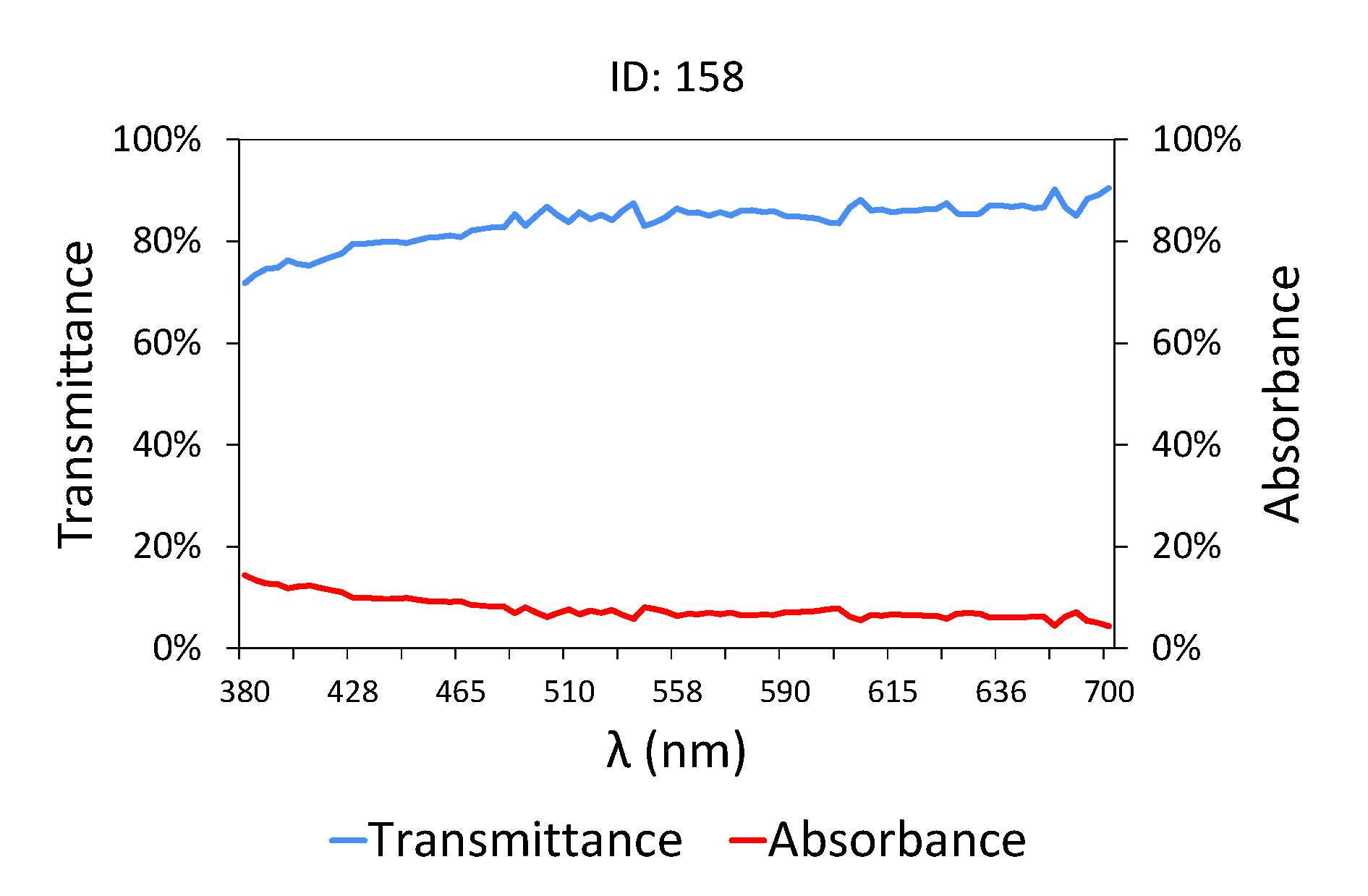
In the case of treated water (
Figure 3 and
Table 3), that is, effluent water obtained at the treatment plant outlet, the transmittance values are much higher than those shown in
Figure 2, as the pollutant load is low in terms of COD, BOD
5 [
71] and TSS. The water at the outlet of the treatment plant has a very high level of transmittance, close to 90% between 445 and 700 nm, where it behaves horizontally, unlike raw water (
Figure 2) where the transmittance values seemed to stabilize from 558 nm. Furthermore, the changes in the slope of the graph are only evident in the area close to ultraviolet/blue, given that this is where organic matter is most sensitive.
3.2. Regression Models
To find the relations between the contaminating parameters and the spectrophotometric data [
8,
17], two different approaches have been proposed: one based on MLR analysis [
72] and the other by calculating GA [
73]. To simplify the equations shown, the following nomenclature is used:
T is transmittance,
A is absorbance and the sub-index indicates the wavelength used for its calculation, for instance
T380 details that this is the transmittance value measured at 380 nm.
It is necessary to emphasize that the coefficients of the different models presented are specific for the device and the wastewater samples used for its calculation. Therefore, these coefficients should be adjusted to the characteristics of the equipment and the peculiarities of the water in the area where the analysis is carried out.
3.2.1. Multivariate Linear Regressions
Multivariate linear regression models [
74,
75,
76] provide correlations from a set of input variables. However, this method is only valid for datasets that follow a normal distribution [
74] (or can be transformed into one). Initially, the tests focused on finding such expressions for a dataset composed of both raw and treated water samples. However, the degree of variability between the two subsets of data composed of both raw and treated water samples was so high that the resulting datasets did not follow a normal distribution, nor was normalization possible despite eliminating outliers.
To illustrate this point more clearly,
Figure S1 presents histograms of combined raw and treated water samples for all of the pollutant parameters under study, where each of the histograms shown contains two differentiated zones: one zone on the right that has an approximately normal distribution, which corresponds to the raw water data, and a dominant class (or classes) in terms of frequency in the left region, which corresponds to the treated water samples. This is especially visible in
Figure S1a–c,f. Therefore, the combination of raw and treated water data cannot be used for the development of MLR models since they do not follow a normal distribution.
The studies carried out showed that it is only possible to apply this type of model achieving an acceptable minimum degree of adjustment when calculating COD, BOD
5 and TSS corresponding to raw water. The rest of the parameters, namely P, TN and NO
3−N, cannot be calculated using that method, since, in most cases, either the data could not be standardized or the resulting model had a low level of correlation (lower 50%). The different multivariate linear regression models obtained for the calculation of COD, BOD
5 and TSS for wastewater (raw water) are shown in the following subsections. The results of the normality tests using the Kolmogorov–Smirnov and Shapiro–Wilk tests as well as the atypical ones detected are shown in
Table S1.
Chemical Oxygen Demand (COD)
The multivariate linear regression model for calculating COD is shown in Equation (3). This model provided a goodness of fit of 77.4% for the training data. The number of samples used for the calculation of the MLR model was 101, out of a total of 108 samples, after eliminating outliers. From this, 69 samples were used in developing the model, while the remaining samples were used for testing it.
c0 = 844.247657
c1 = 1752.845
c2 = 5665.418
c3 = 7189.785
c4 = 8046.775
Figure 4 shows a comparison between the COD values obtained at the wastewater treatment plant (blue), the COD values provided by the model shown in Equation (3), both using the training data (red), i.e., the dataset used for building the model up, and the testing dataset (yellow), which is the data that were been used for developing the model.
In general terms, the calculated values are quite close to the expected data.
Biological Oxygen Demand at 5 Days (BOD5)
The multivariate linear regression model for calculating BOD
5 is shown in Equation (2). This model provided a goodness of fit of 61.9% for the training data. The model has a low adjustment compared to the previous model. The number of samples used for the calculation of the model was 86, out of a total of 108 samples, after eliminating outliers, so that 70 samples were used in developing the model, while the remaining samples were used for testing it.
c0 = 2171.855
c1 = 7898.15
c2 = 4755.737
c3 = 2906.184
Figure S2 shows a comparison between the BOD
5 values provided by the model in Equation (4) (red, the dataset used for building the model up, and yellow, the testing dataset) and the values obtained at the wastewater treatment plant (blue).
In general terms, the calculated values present an appreciable scatter when compared with the reference data.
Total Suspended Solids (TSS)
The multivariate linear regression model for calculating TSS is shown in Equation (5). This model provided a goodness of fit of 72.2% for the training data. The number of samples used for the calculation of the MLR model was 92, out of a total of 108 samples, after eliminating outliers, so that 69 samples were used in developing the model, while the remaining samples were used for testing it.
c0 = 2428.586
c1 = 5060.755
c2 = 2928.048
Figure S3 shows a comparison between the TSS values provided by the model in Equation (5) (red, the dataset used for building the model up, and yellow, the testing dataset) and the values obtained at the wastewater treatment plant (blue). As can be seen, in general terms, the model fits the expected TSS values quite well.
As was already observed in the MLR of the COD, the calculated values are quite close to the expected data.
To show the relationship between each of the variables used in the respective models (Equations (3)–(5)) with respect to the pollutant parameter under study, the
Supplementary Materials include scatter diagrams for COD (
Figure S4), BOD5 (
Figure S5) and TSS (
Figure S6).
3.2.2. Genetic Algorithms
The MLR models, as shown in the previous section, might be suitable to quantify the pollution load influent to the WWTP, i.e., raw wastewater, in terms of COD and TSS. In contrast, MLR models have difficulties in modeling the behavior of samples with low COD and BOD
5 levels, i.e., COD lower than 55 mg/L and BOD
5 lower than 15 mg/L, which is the WWTP effluent. This is due to the fact that the transmittance/absorbance fluctuations in the UV–near visible spectrum are less significant than those observed in the wastewater. This is observed in
Figure 3, where the transmittance graph resembles an almost horizontal line.
We aimed to develop a model that could be applied to both raw and treated water, which would overcome the limitations of MLR models and have a good level of accuracy in the estimates. For that reason, we developed a genetic algorithm, more specifically symbolic regression models. For each of the calculated models, 66% of the samples were used as the training data and the remaining 34% were used to validate the data. It is necessary to highlight that the data used for training and testing were selected randomly.
The following subsections show the results obtained by the algorithms, for each of the parameters analyzed: COD, BOD5, TSS, P, TN and NO3−N. Each of them is followed by its correlation formula, as well as a comparison with the expected values of the polluting parameters.
Chemical Oxygen Demand (COD)
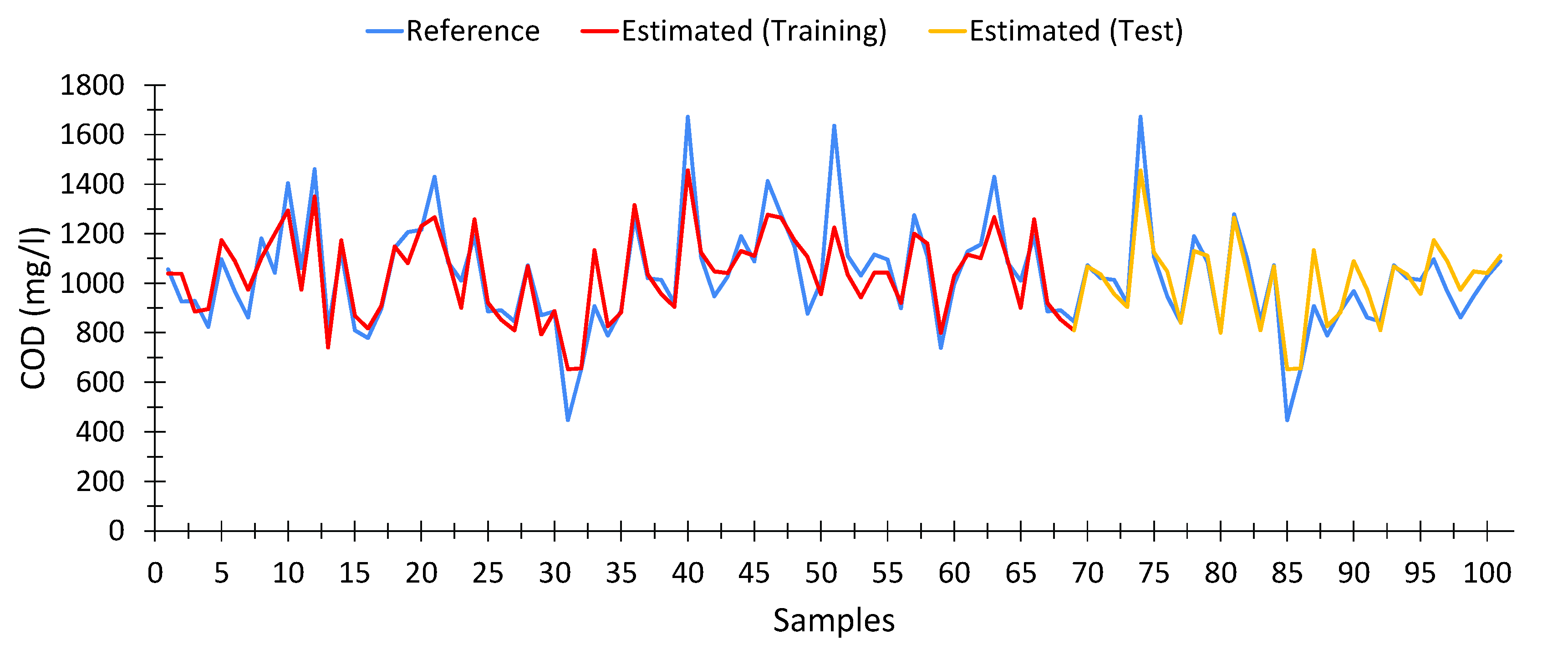
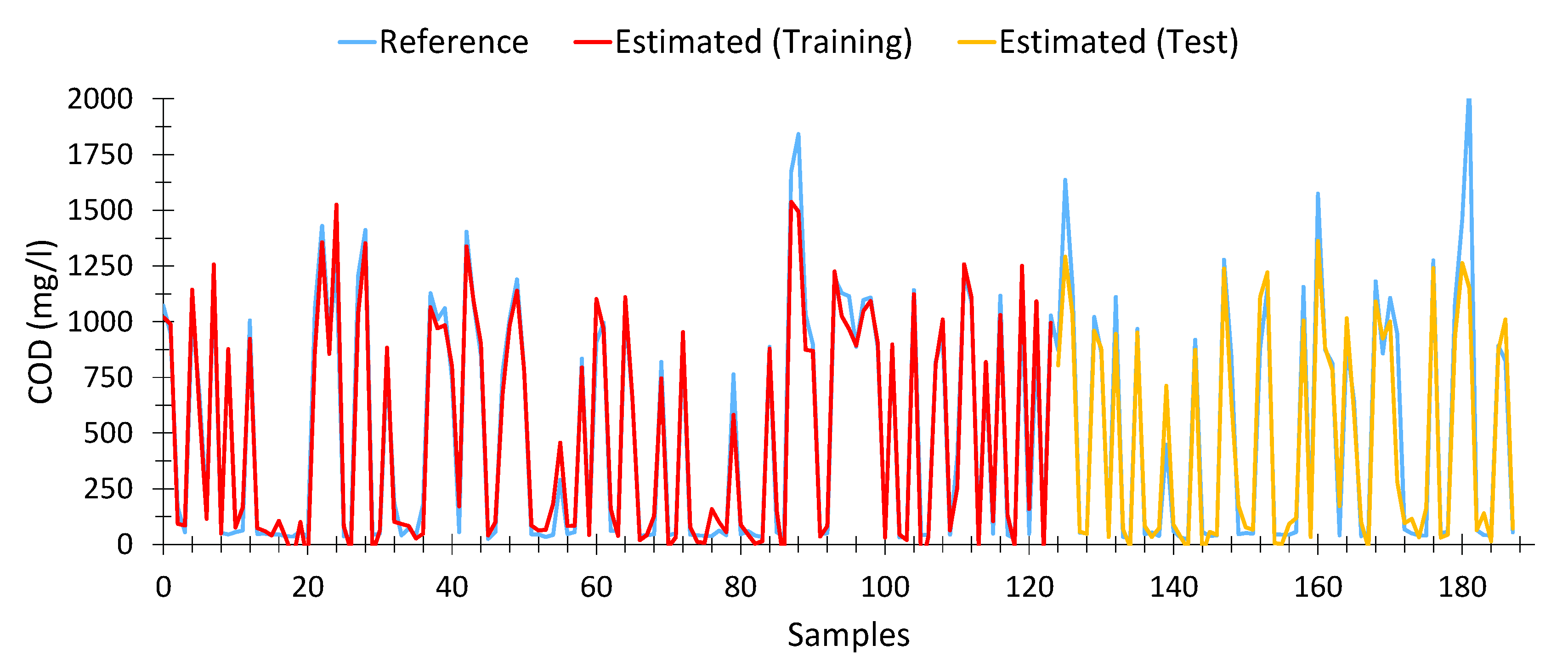
The model for calculating COD from spectrophotometric data is shown in Equation (6). This model presented an average Pearson goodness-of-fit for nonlinear regressions of 90.95%, with a similar adjustment in the training data (95.07%) and the test data (90.93%). In total, 188 samples out of 196, taken from different treatment plants and days, as well as input water (raw water) and output water (treated water), were used for the calculation. The optimal model was achieved in the generation number 84 of a maximum of 100.
c0 = 2.4268
c1 = 2.7910
c2 = 2.5317
c3 = 2.6341
c4 = 2.3278
c5 = 2.6879
c6 = 2.4569
c7 = 2.7717
c8 = 1191.8
c9 = −263.45
This model is based on eight wavelengths for its calculation, namely 380, 425, 445, 520, 521, 570, 575 and 594 nm, more specifically from the absorbance data. However, not all variables (wavelengths) are equally relevant. As shown in
Table 4, 380, 425, 445 and 594 nm are the most relevant variables, with an impact factor close to 17%, while the remaining variables are at around 5%.
It is important to note that the wavelengths with the highest impact index were those belonging to the violet zone of the visible spectrum (380–450 nm), which was to be expected, since organic matter is far more sensitive to those wavelengths. Likewise, it was also observed that the wavelengths close to red showed a greater interaction with the water samples. This suggests that the use of near-infrared wavelengths would provide better characterization of the samples.
As shown in
Figure 5, the estimates provided by the model (both for training (red) and test (orange) data) fit precisely with the expected results (Blue). We can see that for very high values of COD (>1600 mg/L) the estimates tend to be lower than expected. However, the results could be adequate to provide an early warning system. However, at low values of COD [
77], the model is able to provide a fairly certain estimation from spectrophotometric data, which was not possible with linear models.
Table A1 in
Appendix B shows 15 random records, which include the absorbance values obtained for each of the variables used in the model (Equation (6)), as well as the expected COD values (Reference) and those calculated by the model (Estimated).
It can be seen that the results calculated are very similar to those expected, even when the COD level is low. The model obtained by means of the genetic algorithm was able to precisely estimate COD values from the data provided by the spectrophotometer.
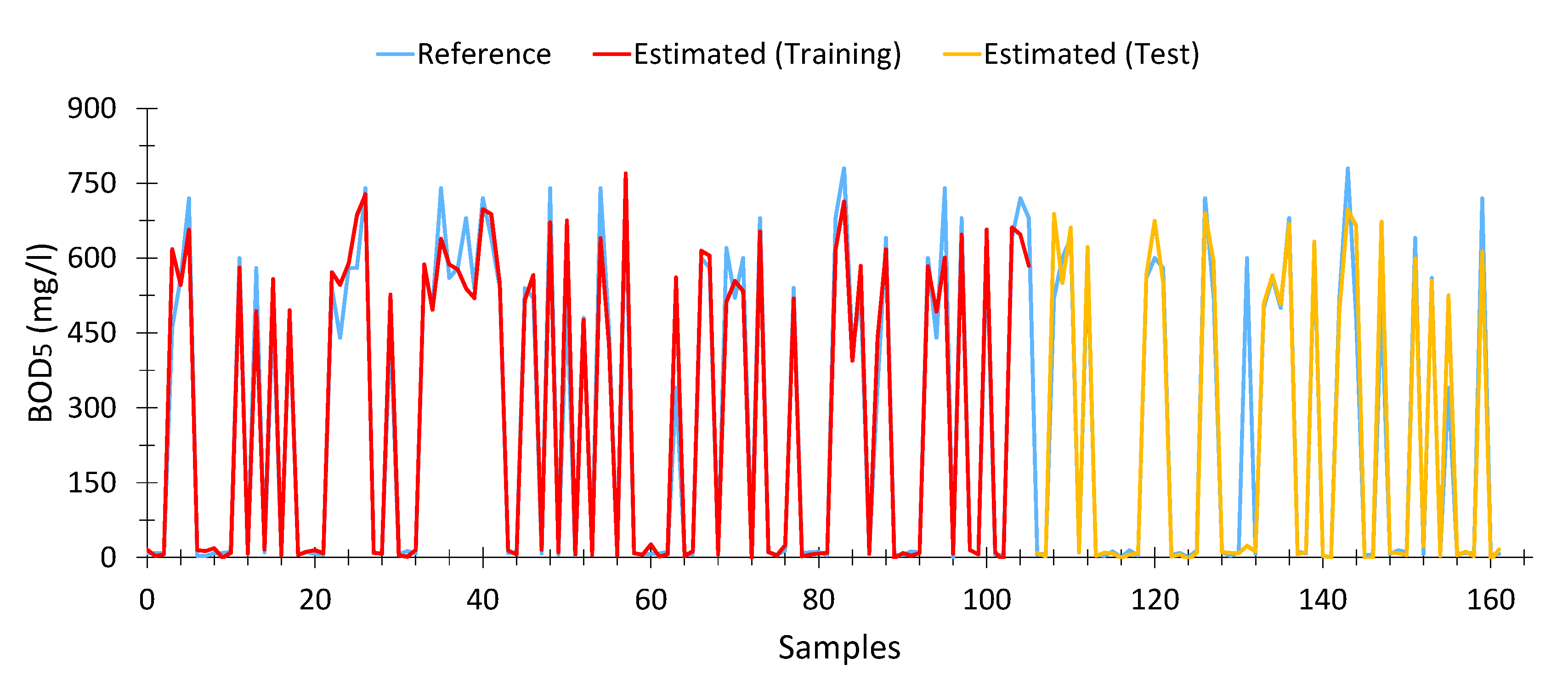
Biological Oxygen Demand at 5 Days (BOD5)
To calculate the model for BOD
5, 162 samples were used out of a total of 196 samples after eliminating outliers—a lower number than before—due to two aspects: the existence of outliers and measurements where BOD
5 data were not available. The calculated model is shown in Equation (7). This model showed an average Pearson goodness-of-fit of 90.71% (training data) and 90% for test data (88.23% average). In addition, the model is valid for water samples with high levels of pollution (raw water) as well as with low levels of pollution (treated water). The optimal model was achieved in the 98th generation.
c0 = 2.0733
c1 = 1.3974
c2 = −1.0226
c3 = 1.2453
c4 = 1.3974
c5 = −0.1356
c6 = −1.0226
c7 = 1.2453
c8 = −10078
c9 = −18.784
This model is based on five wavelengths for its calculation: 415, 445, 574, 585 and 655 nm. However, not all variables (wavelengths) are equally relevant. As can be seen in
Table 5, the most relevant wavelengths are those closest to the violet area [
78], although the wavelengths close to red have a similar level of importance, although in smaller proportions.
Figure 6 shows the estimations of the genetic algorithm. As can be seen, the adjustment is acceptable, although in general terms the results seem to be a little lower than expected, but this fluctuation is not significant.
Table A2 (
Appendix B) shows 15 records taken at random, where the results obtained by the model are very similar to those that were expected. Each record contains the spectrophotometric data as well as the expected (reference) values calculated by the model.
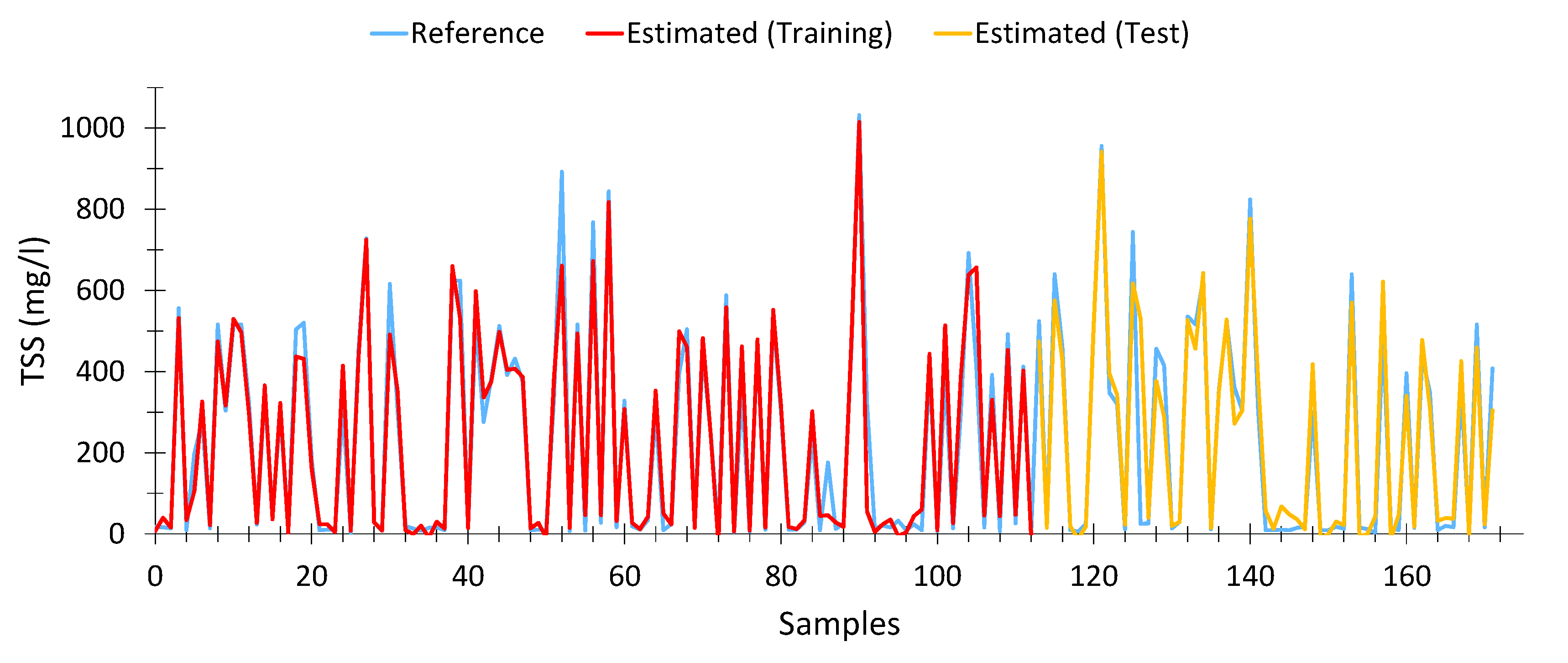
Total Suspended Solids (TSS)
Equation (8) shows the model calculated for total suspended solids. This model presented an average Pearson goodness-of-fit of 87.47% (94.67% with the training data and 90% with the test data). In total, 172 samples were used out of the 196 samples, after eliminating outliers.
c0 = −0.062545
c1 = 2.6249
c2 = 3.4131
c3 = 2.5468
c4 = 3.3361
c5 = 0.46423
c6 = 782.89
c7 = −779.73
The model makes use of six variables (wavelengths): transmittance at 380, 485, 558, 565 and 632 nm and absorbance at 574 nm. However, the most relevant are 380 and 485 nm, as shown in
Table 6. Likewise, we observe that, as wavelengths approach the infrared spectrum, the relative weight of these variables decreases significantly, as is the case with 632 nm.
This shows that particles in suspension are far more sensitive to wavelengths close to violet than to other wavelengths.
Figure 7 shows the results obtained with the calculated model. As can be seen, the fit is adequate, even at high TSS levels.
Similar to the previous cases,
Table A3 (
Appendix B) shows 15 cases chosen at random, in order to verify the good performance of the model, even at low levels of TSS.
Phosphorus (P)
The model calculated for P is shown in Equation (9). The model presented an average Pearson goodness-of-fit of 74.01% (74.28% with the training data and 78.33% with the test data), with the optimum being raised at generation 38 of a maximum of 100. In total, 175 data were used for its calculation.
c0 = 1.53
c1 = 0.8773
c2 = 1.1618
c3 = 1.5294
c4 = 0.8773
c5 = 2.2034
c6 = 1.1618
c7 = −40.766
c8 = 9.0573
The calculated model uses five wavelengths: 425, 430, 450, 585 and 650 nm. Once again, the most representative wavelengths were those closest to the violet zone [
79], as shown in
Table 7. As with the total suspended solids model, the weight of the wavelengths decreases as it approaches the infrared portion of the spectrum.
The model generated to estimate phosphorus levels from spectrophotometric data has a lower adjustment compared to the previous models and presents systematic inaccuracies for higher concentrations. The calculated model was only able to accurately estimate
p values lower than or equal to 9 mg/L. This characteristic can be seen in
Figure S7, where the estimated values are never higher than that value.
Table A4 (
Appendix B) shows 15 cases chosen at random, in order to verify the performance of the model.
Total Nitrogen (TN)
The model for Total Nitrogen (TN) is shown in Equation (10). This model had an average Pearson goodness-of-fit of 79.93% (85.91% with the training data and 85.91% with the test data), having been calculated from 175 samples out of the total of 196 after eliminating outliers. The optimum was raised at generation 87.
c0 = 1.3315
c1 = 0.85214
c2 = 2.1725
c3 = 1.6762
c4 = 1.4023
c5 = 0.85214
c6 = 2.1725
c7 = 1.6605
c8 = −1271.6
c9 = 83.172
The model makes use of six wavelengths: 500, 510, 557, 585, 640 and 655 nm. As shown in
Table 8, the most representative wavelengths used to calculate the nitrogen content of water were those closest to infrared. This has already been highlighted in [
80], where nitrogen has a higher correlation with wavelengths close to the infrared spectrum [
81].
Figure S8 shows the results provided by the model described in 10. As can be seen, the formula works well within a certain range of nitrogen values between 20 and 75 mg/L, but worsens slightly outside that range, albeit not significantly.
Within that range, the results provided by the model were very close to the reference values, as shown in
Table A5 (
Appendix B).
Nitrate Nitrogen (NO3−N)
Nitrogen nitrate in water can be calculated from Equation (11). The model presented an average Pearson goodness-of-fit of 81.26% (81.26% with the training data and 83.46% with the test data). In total, 175 samples were used for calculation out of 196 samples after eliminating outliers. The optimum was raised at generation 81 of 100.
c0 = 2.2576
c1 = 2.2576
c2 = −0.53193
c3 = 1.5017
c4 = 0.66989
c5 = 2.277
c6 = −0.53193
c7 = −0.50608
c8 = −0.010536
c9 = −0.12637
The model uses the following six wavelengths: 385, 428, 560, 607, 624 and 645 nm. The tests showed that NO
3−N has a higher correlation with wavelengths close to 600 nm, as shown in
Table 9.
Figure S9 shows the results obtained for different water samples. Considering that the vertical scale in the figure is shown in 2 mg/L intervals, the discrepancies between the calculated values and the reference values are not significant.
Table A6 (
Appendix B) shows 15 cases chosen at random, where the high degree of similarity between the data provided by the model and the values calculated in the wastewater treatment plants can be observed.
3.2.3. Decision Support System Proposal
To carry out an in-depth analysis of the different models calculated, the RMSE and Error Rate E(%) were calculated following Equations (1) and (2), respectively. The results are shown in
Table 10.
As shown in
Table 10, the COD error value provided by the MLR model (−0.096%) is lower than that obtained by the genetic algorithm (−2.374%). Nevertheless, we must take into account that a different number of samples was used; GA takes treated water into account; thus, although it is true that the MLR model showed better performance than that provided by the genetic algorithm, its use is limited to raw water.
Thus, if the samples which we seek to obtain the COD value for are only samples of raw water, then the MLR model presents the best results. However, if we want to carry out the study on both types of water (raw and treated), then the genetic algorithm must be used to calculate the COD. The genetic algorithm presented the best performance for the remaining parameters.
Looking into the contribution of the wavelengths to the statistical models, not all wavelengths have the same weight in the models, as shown in
Table 4,
Table 5,
Table 6,
Table 7,
Table 8 and
Table 9. In general terms, those wavelengths closer to violet have a greater weight, which is understandable considering that organic matter reacts more to UV than to other wavelengths. On the other hand, wavelengths close to IR also have a greater importance in the calculation of inorganic parameters such as TN.
In addition, although in general terms the models calculated by means of the genetic algorithms present a better performance, it is necessary to emphasize that these models make use of a greater number of variables (wavelengths) than the models of linear regression. This implies a greater time of analysis and an increase of the load of the system as well as the price of the equipment since more LEDs is necessary. Therefore, the choice of the model will depend on the application.
Table 11 shows the different wavelengths used for the calculation of the six pollutant parameters, where each cell shows the degree of importance of that wavelength in its calculation, accompanied by a color code, for greater clarity of the reader: green (high relevance), blue (medium-high relevance), orange (medium-low relevance) and red (low relevance). The coefficients shown were determined automatically by the SPSS software and gpLearn from the
P-value of the variables introduced in the different models.
As shown in
Table 11, the contaminating parameters related to organic matter, such as COD and BOD5, show a greater interaction with wavelengths close to violet and with a lower extent with wavelengths in the order of 500–550 nm (green).
On the other hand, the parameters more related to inorganic matter such as total nitrogen (TN) are more sensitive to wavelengths close to the infrared (IR); in fact, the TN is calculated using NIRS techniques (near infrareds) [
82,
83].
At this point, it is necessary to make a comparison between the wavelengths present in the MLR and GA models. As shown in
Table 11, the wavelengths selected by both methodologies are similar, especially in the ultraviolet zone, where, for example, the wavelength of 380 nm is present for both COD and BOD
5 in both types of models (MLR and GA). On the other hand, it is necessary to take into account that GA models are valid for both raw and treated water and therefore it is logical to think that the number of wavelengths used is greater than that required to model only raw water. Despite this, there are similarities between both types of models.
4. Conclusions
In this paper, we show different models that enable us to estimate the concentration of COD, BOD5, TSS, P, TN and NO3−N from the absorbance and transmittance measures of the water samples, within the range of 380–700 nm. These models can be used to estimate the pollutant load of both the incoming water (raw water) and the outgoing water (treated water), without the need for any pre-treatment or chemicals.
The research focused on two types of models: multivariate linear regression and genetic algorithm. The tests carried out determined that the models calculated by means of genetic algorithms are able to obtain valid estimates principally for five of the pollutants under study (COD, BOD5, TSS, TN and NO3−N), including both raw and treated waste water in the adjustments, with an error rate below 4% in all the models. In the case of the MLR models, their adequacy is limited to COD and TSS, while BOD5 presents a poor fit. In contrast to GA, the MLR models presented better error rates than those calculated by genetic algorithms, with an error rate of less than 0.5% for COD and TSS. However, MLR models are limited to raw water samples. The variability of wastewater samples makes it difficult for MLR models to find a single valid model for both influent (raw water) and effluent (treated) wastewater. However, models calculated by means of genetic algorithms have proven to be reliable enough to find common patterns among the different types of samples, in order to achieve a valid calculation model for all types of wastewater (raw and treated).
The current research also provides a clearer view of the effect that each of the UV–near visible and visible wavelengths (380–700 nm) have on the estimation of each of the polluting parameters. As shown in
Table 11, the wavelengths having the greatest effect on the calculation are those corresponding to the UV–near visible (380–400 nm) and near-infrared (600–700 nm) zones, with a relevance (impact) of 17–20% in the model calculation, while the zone between 500 and 600 nm is the least relevant, with an impact of around 5%, albeit with some exceptions, such as TSS (around 10%).
COD, BOD5, TSS and P depend mainly on the UV zone for their calculation, representing (in the case of models calculated with the GA) around 52%, 40%, 70% and 40%, respectively. On the other hand, TN and NO3−N depend mainly on the IR zone.
In this research work, a completely different approach was sought to what is followed by systems such as those described in [
59,
60,
61,
62], which base their operation on the analysis of the turbidity of wastewater samples, that is, on a turbidimeter. A turbidimeter analyzes the samples at a single wavelength (typically belonging to the infrared spectrum). In contrast, the system developed and described in this manuscript makes use of 81 different wavelengths. This allows a much more precise knowledge of the physical-chemical and bacteriological properties of the samples, since wavelengths close to UV are of great importance to know the behavior of organic matter, while wavelengths close to red (or infrared) enable analyzing the behavior of inorganic matter with high precision. Therefore, the use of multiple wavelengths makes it possible to obtain adequate estimates of the pollution load of wastewater.
This research can serve as a starting position for future continuous real-time monitoring of the whole sanitation system that includes the deployment of simpler, smaller and more cost-effective equipment for the study of the pollutant load in sewage networks, capable of obtaining valuable information from the spectrophotometry-based statistical models and providing early warning. This distribution of this equipment along the networks can be especially useful during rain episodes, when the pollution load of sanitation networks tends to rise, and represents a danger to the environment. Therefore, having rapid information on this type of parameters is essential for preventing and reducing environmental disasters.

 ,
, 


