Geosynchronous Satellite GF-4 Observations of Chlorophyll-a Distribution Details in the Bohai Sea, China

Abstract
1. Introduction
2. Data and Method
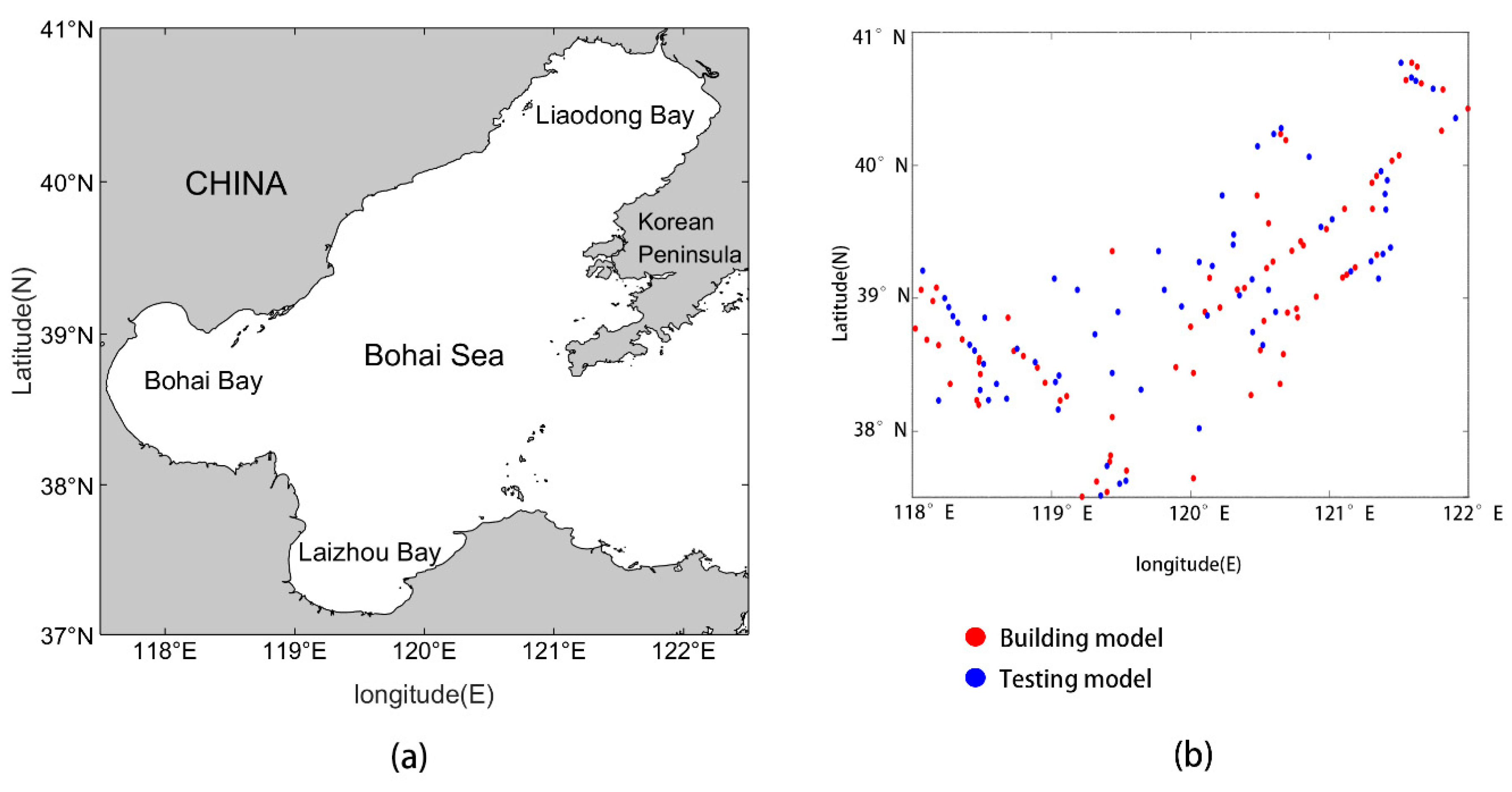
2.1. Study Area
2.2. Satellite Data
2.3. In Situ Data
2.4. Data Processing
2.4.1. Radiation Calibration
2.4.2. Atmospheric Correction
2.4.3. Geometrical Correction of Image
2.4.4. Inversion Modeling Method
3. Result
3.1. Correlation Analysis of Panchromatic Multispectral Sensor (PMS) Inversion Algorithm
Sensitive Bands of Chlorophyll-A (Chla)
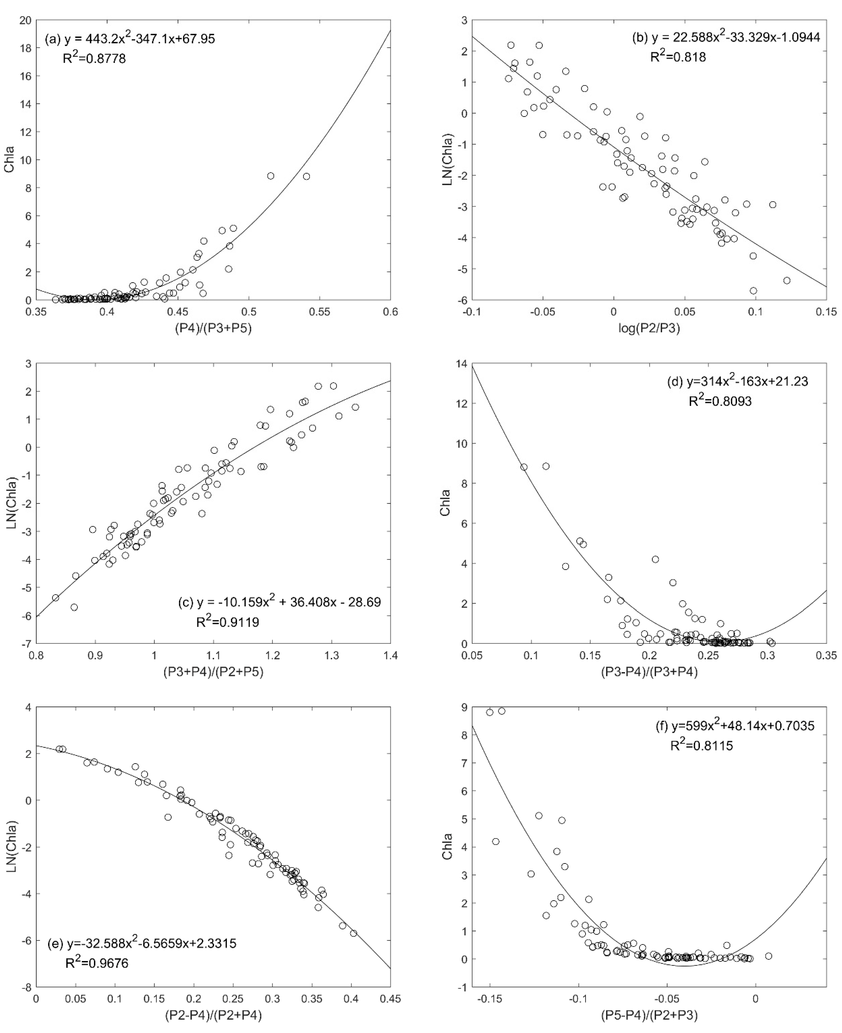
3.2. Band Combination
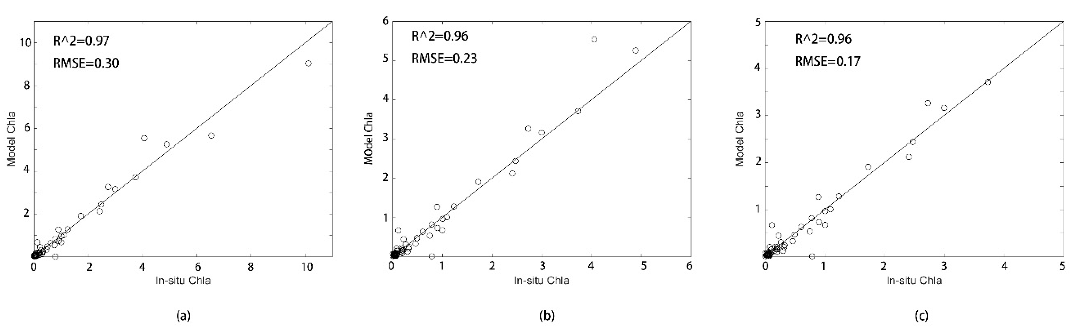
3.3. Model Building
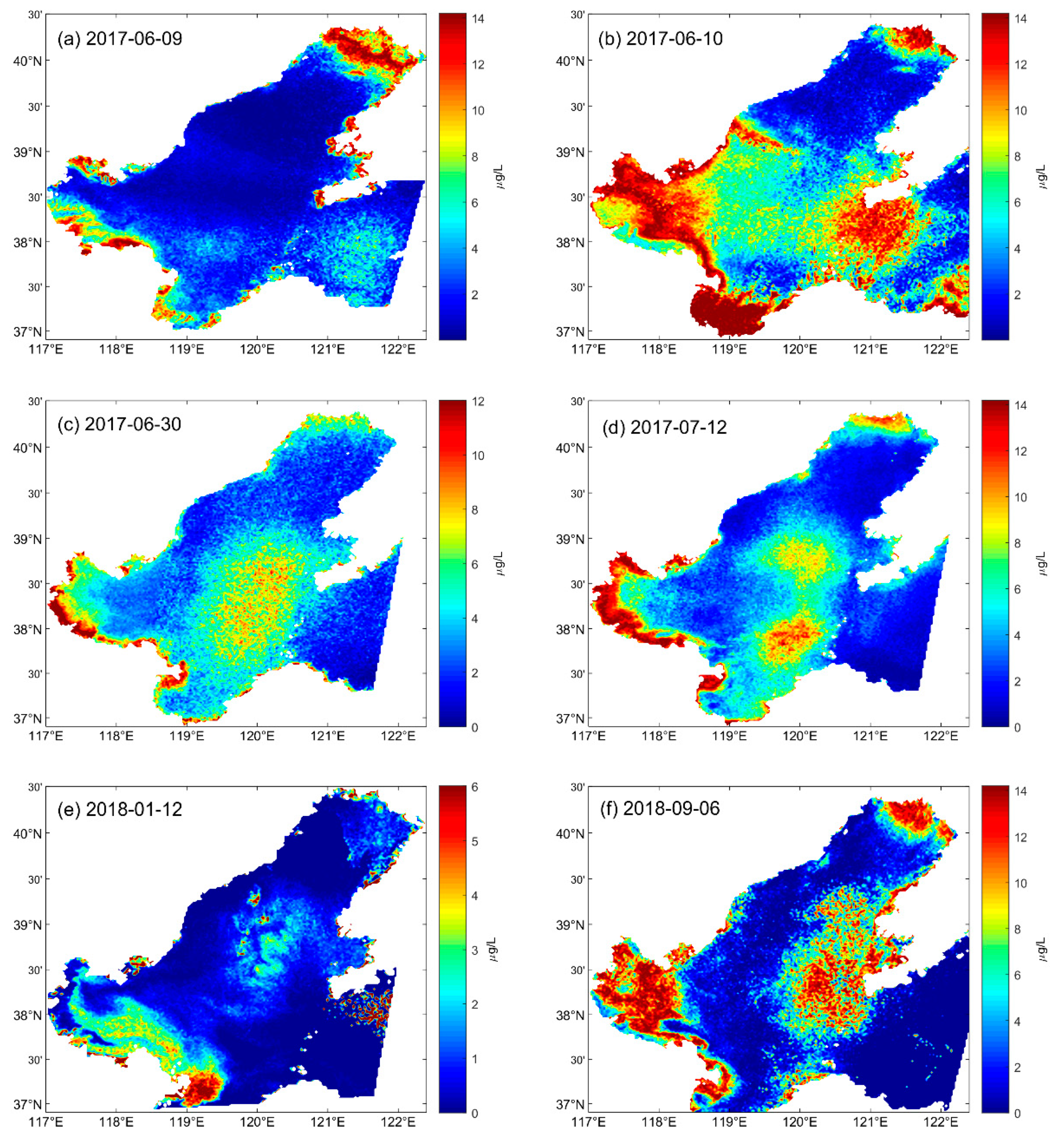
3.4. Details of Short-Term Change in Chla Concentration
4. Discussion
4.1. Feasibility and Necessity of the Gaofen-4 (GF-4) PMS-1 Model in the Bohai Sea
4.2. Factors Affecting Chla Concentration in the Bohai Sea
5. Conclusions
Author Contributions
Funding
Acknowledgments
Conflicts of Interest
References
- Wang, Y.; Jiang, H.; Zhang, X.; Jin, J. Satellite remotely-sensed analysis of temporal-spatial variations of chlorophyll-a concentration in South China Sea. In Proceedings of the International Conference on Geoinformatics, Shanghai, China, 24–26 June 2011; pp. 1–5. [Google Scholar]
- Bin, Z.; Ya-Rong, Z.; Zhen-Gang, J. Analysis of characteristics of seasonal and spatial variations of sst and chlorophyll concentration in the bohai sea. Adv. Mar. Sci. 2015, 23, 487–492. [Google Scholar]
- Mueller, J.L. Effects of water reflectance at 670 Nm on coastal zone color scanner (CZCS) aerosol radiance estimates off the coast of central california. In Proceedings of the Ocean Optics VII, Monterey, CA, USA, 27 September 1984. [Google Scholar]
- Wang, M.; Cheng, Y.; Long, X.; Yang, B. On-orbit geometric calibration approach for high-resolution geostationary optical satellite gaofen-4. Int. Arch. Photogramm. Remote Sens. Spat. Inf. Sci. 2016, XLI-B1, 389–394. [Google Scholar]
- Rietbroek, R.; Brunnabend, S.E.; Kusche, J.; Schroeter, J.; Dahle, C.; Uebbing, B. Breaking down Global and Regional Sea Level Budgets: What Satellite Observations can tell us. In Proceedings of the EGU General Assembly, Vienna, Austria, 12–17 April 2015. [Google Scholar]
- Wang, L.; Zhao, D.; Yang, J.; Chen, Y. Retrieval of total suspended matter from MODIS 250 m imagery in the Bohai Sea of China. J. Oceanogr. 2012, 68, 719–725. [Google Scholar] [CrossRef]
- Fearns, P.R.C.S.; Lynch, M.J. Retrieval of chlorophyll concentration via inversion of ocean reflectance: A modeling approach. In Proceedings of the SPIE—The International Society for Optical Engineering, Halifax, NS, Canada, 6 February 1997. [Google Scholar]
- Sun, X.; Shen, F.; Brewin, R.J.; Liu, D.; Tang, R. Twenty-year variations in satellite-derived chlorophyll-a and phytoplankton size in the Bohai Sea and Yellow Sea. J. Geophys. Res. Oceans 2019, 124, 8887–8912. [Google Scholar] [CrossRef]
- De-Juan, J.; Hua, Z. Analysis of spatial and temporal characteristics of chlorophyll-a concentration and red tide monitoring in Bohai Sea. Mar. Sci. 2018, 42, 23–31. [Google Scholar]
- Zhu, W.; Lei, H. Remote sensing retrieval for Chlorophyll-a and Suspended Matter Concentration of Longyangxia Reservoir based on landsat OLI data. IOP Conf. Ser. Earth Environ. Sci. 2019, 310, 022037. [Google Scholar] [CrossRef]
- Giteloson, A.A.; Kondratyev, K.Y. Optical models of mesotrophic and eutrophic water bodies. Int. J. Remote Sens. 1991, 12, 373–385. [Google Scholar] [CrossRef]
- Keiner, L.E.; Yan, X.-H. A neural network model for estimating sea surface chlorophyll and sediments from thematic mapper imagery. Remote Sens. Environ. 1998, 66, 153–165. [Google Scholar] [CrossRef]
- Shu, X.Z.; Kuang, D.B. New algorithm to estimate chlorophyll-a concentration from the spectral reflectance of inland water. In Proceedings of the SPIE Hyperspectral Remote Sensing and Application, Asia-Pacific Symposium on Remote Sensing of the Atmosphere, Environment, and Space, Beijing, China, 14–17 September 1998; Volume 3502, pp. 254–258. [Google Scholar]
- Mishra, S.; Mishra, D.R. Normalized difference chlorophyll index: A novel model for remote estimation of chlorophyll-a concentration in turbid productive waters. Remote Sens. Environ. 2012, 117, 394–406. [Google Scholar] [CrossRef]
- Marghany, M.; Hashim, M. MODIS satellite data for modeling chlorophyll-a concentrations in Malaysian coastal waters. Am. J. Neuroradiol. 2010, 5, 1489–1495. [Google Scholar]
- Youchuan, W.; Jiajie, H.; Liangming, L. Theory and implementation of chlorophyll inversion algorithm for two types of water bodies based on modis data. Wuhan Univ. J. Inf. Sci. 2007, 32, 572–575. [Google Scholar]
- Pan, B.L.; Wang, X.H.; Zhu, J.; Yi, W.N. Polarized Hyperspectral Inversion Model of Chlorophyll in the Lake Water. Spectrosc. Spectral Anal. 2013, 33, 1665–1669. [Google Scholar]
- He, Z.; Xiao-Shen, Z. Study on red tide remote sensing monitoring in the bohai sea in 2014. Mar. Bull. 2017, 19, 37–51. [Google Scholar]
- Kuhn, C.; de Matos Valerio, A.; Ward, N.; Loken, L.; Sawakuchi, H.O.; Kampel, M.; Richey, J.; Stadler, P.; Crawford, J.; Striegl, R.; et al. Performance of Landsat-8 and Sentinel-2 surface reflectance products for river remote sensing retrievals of chlorophyll-a and turbidity. Remote Sens. Environ. 2019, 224, 104–118. [Google Scholar] [CrossRef]
- Li, J.; Gao, M.; Feng, L.; Zhao, H.; Shen, Q.; Zhang, F.; Wang, S.; Zhang, B. Estimation of chlorophyll-a concentrations in a highly turbid eutrophic lake using a classification-based MODIS land-band algorithm. IEEE J. Sel. Topics Appl Earth Observ. Remote Sens. 2019, 12, 3769–3783. [Google Scholar] [CrossRef]
- Chong, D.; Li, H.J.; Fan, S.; Li, J.J.; Wang, J.; Zhang, S.Q. Inversion of chlorophyll-a concentration in nine plateau lakes in Yunnan based on MODIS data. Chin. J. Ecol. 2017, 36, 277–286. [Google Scholar]
- Tanré, D.; Kaufman, Y.J.; Herman, M.; Mattoo, S. Remote sensing of aerosol properties over oceans using the MODIS/EOS spectral radiances. J. Geophys. Res. Atmos. 1997, 102, 16971–16988. [Google Scholar] [CrossRef]
- Zheng, G.X.; Song, J.M.; Dai, J.C.; Wang, Y.M. Distribution characteristics of chlorophyll-a and carbon sequestration intensity of phytoplankton in the southern yellow sea. Acta Oceanol. Sin. Chin. Ed. 2006, 3, 111–120. [Google Scholar]
- Yun, M.; Angang, L.; Yafei, L.I.U.; Dongliang, Z. Effects of coastal topography changes on tidal wave systems and tidal properties in the Bohai Sea. J. Ocean Univ. China Nat. Sci. Ed. 2015, 45, 1–7. [Google Scholar]
- Wang, M.; Cheng, Y.; Tian, Y.; He, L.; Wang, Y. A new on-orbit geometric self-calibration approach for the high-resolution geostationary optical satellite gaoFen4. IEEE J. Sel. Topics Appl. Earth Observ. Remote Sens. 2018, 11, 1670–1683. [Google Scholar] [CrossRef]
- Li, F.; Xin, L.; Guo, Y.; Gao, D.; Kong, X.; Jia, X. Super-Resolution for GaoFen-4 Remote Sensing Images. IEEE Geosci. Remote Sens. Lett. 2018, 15, 28–32. [Google Scholar] [CrossRef]
- Xu, J.; Liang, Y.; Liu, J.; Huang, Z. Multi-frame super-resolution of gaofen-4 remote sensing images. Sensors 2017, 17, 2142. [Google Scholar]
- Liu, Y.; Yao, L.; Xiong, W.; Zhou, Z. GF-4 satellite and automatic identification system data fusion for ship tracking. IEEE Geosci. Remote Sens. Lett. 2018, 16, 281–285. [Google Scholar] [CrossRef]
- Chen, Y.; Sun, K.; Li, D.; Bai, T.; Huang, C. Radiometric cross-calibration of GF-4 PMS sensor based on assimilation of landsat-8 OLI images. Remote Sens. 2017, 9, 811. [Google Scholar] [CrossRef]
- Ming, X. A new generation of geostationary satellites. Foreign Space Dyn. 1986, 11, 25–26. [Google Scholar]
- Lingjie, M.; Ding, G.; Menghui, T.; Qi, W. Development status and prospects of high-resolution imaging satellites in geostationary orbit. Spacecr. Rec. Return Remote Sens. 2016, 37, 1–6. [Google Scholar]
- Guohong, F.; Jingfei, Y. A two-dimensional numerical model of the tidal motions in the Bohai sea. Chinese J. Oceanol. Limnol. 1985, 2, 135–152. [Google Scholar] [CrossRef]
- Wenling, L.; Xiaoshen, Z.; Xiang, A.; Jing, W. Research on inversion methods of chlorophyll concentrations in Bohai Sea. In Proceedings of the Wri World Congress on Computer Science & Information Engineering, IEEE Computer Society, Los Angeles, CA, USA, 31 March–2 April 2009. [Google Scholar]
- Liu, X.; Sun, L.; Yang, Y.; Zhou, X.; Wang, Q.; Chen, T. Cloud and cloud shadow detection algorithm for gaofen-4 satellite data. Acta Optica Sin. 2019, 39, 446–457. [Google Scholar]
- Wang, M.; Cheng, Y.; Chang, X.; Jin, S.; Zhu, Y. On-orbit geometric calibration and geometric quality assessment for the high-resolution geostationary optical satellite GaoFen4. ISPRS J. Photogr. Remote Sens. 2017, 125, 63–77. [Google Scholar] [CrossRef]
- Ghimire, P.; Lei, D.; Juan, N. Effect of Image Fusion on Vegetation Index Quality Comparative Study from Gao fen-1, Gaofen-2, Gaofen-4, Landsat-8 OLI and MODIS Imagery. Remote Sens. 2020, 12, 1550. [Google Scholar] [CrossRef]
- Jiabiao, L.; Peiying, L.; Shang, C.; Yijun, Z.; Xiaoguo, Y.; Weidong, J. Standards for Marine Surveys; Standardization in China: Beijing, China, 2011; Volume 2, pp. 34–38. [Google Scholar]
- Qing-Jiu, T.; Lan-Fen, Z.; Qing-Xi, T. Image based atmospheric radiation correction and reflectance retrieval methods. Quart. J. Appl. Meteorol. 1998, 9, 456–461. [Google Scholar]
- Guo, Y.; Zeng, F. Atmospheric correction comparison of spot-5 image based on model flash and model quac. ISPRS Int. Arch. Photogr. Remote Sens. Spat. Inf. Sci. 2012, XXXIX-B7, 7–11. [Google Scholar] [CrossRef]
- Yang, C.; Tang, D.; Haibin, Y.E. A study on retrieving chlorophyll concentration by using gf-4 data. J. Trop. Oceanogr. 2017, 7, 33–39. [Google Scholar]
- Vermote, E.F.; El Saleous, N.; Justice, C.O.; Kaufman, Y.J.; Privette, J.L.; Remer, L.; Roger, J.-C.; Tanre, D. Atmospheric correction of visible to middle-infrared eos-modis data over land surfaces: Background, operational algorithm and validation. J. Geophys. Res. 1997, 102, 17131. [Google Scholar] [CrossRef]
- Wei, Z.; Zhiyuan, Z. Overview of atmospheric correction methods for remote sensing images. Remote Sens. Inf. 2004, 4, 66–70. [Google Scholar]
- Matthew, M.; Adler-Golden, S.; Berk, A.; Felde, G.; Anderson, G.; Gorodetzky, D.; Paswaters, S.; Shippert, M. Atmospheric correction of spectral imagery: Evaluation of the FLAASH algorithm with AVIRIS data. In Proceedings of the IEEE Applied Imagery Pattern Recognition Workshop, Washington, DC, USA, 16–18 October 2003. [Google Scholar]
- Felde, G.W.; Anderson, G.P.; Cooley, T.W.; Matthew, M.W.; Berk, A.; Lee, J. Analysis of Hyperion data with the FLAASH atmospheric correction algorithm. In Proceedings of the IGARSS ’03 IEEE International Geoscience and Remote Sensing Symposium, Toulouse, France, 21–25 July 2003. [Google Scholar]
- Vermote, E.F.; Saleous, N.Z.E.; Justice, C.O. Atmospheric correction of MODIS data in the visible to middle infrared: First results. Remote Sens. Environ. 2002, 83, 97–111. [Google Scholar] [CrossRef]
- Shmirko, K.; Bobrikov, A.; Pavlov, A. Atmospheric correction of satellite data. In Proceedings of the XXI International Symposium Atmospheric & Ocean Optics Atmospheric Physics, Tomsk, Russia, 22–26 June 2015. [Google Scholar]
- Gianinetto, M.; Scaioni, M. Automated geometric correction of high-resolution pushbroom satellite data. Photogr. Eng. Remote Sens. 2008, 74, 107–116. [Google Scholar] [CrossRef]
- Storey, J.C.; Choate, M.J. Landsat-5 bumper-mode geometric correction. IEEE Trans. Geosci. Remote Sens. 2004, 42, 2695–2703. [Google Scholar] [CrossRef]
- Li, Q.; Wenling, L.; Xiaochen, Z. Temporal and spatial variation of chlorophyll concentration in Bohai Sea based on MODIS data inversion. Mar. Bull. 2011, 30, 683–687. [Google Scholar]
- Guoliang, T.; Xiaodong, N.; Fu, S.; Weiling, Z. Estimating chlorophyll concentration in water using spectral data. Environ. Remote Sens. 1988, 1, 71–80. [Google Scholar]
- Lin, Y.; Ye, Z.; Zhang, Y.; Yu, J. Spectral feature analysis for quantitative estimation of cyanobacteria chlorophyll-a. ISPRS-International Archives of the Photogrammetry. Remote Sens. Spat. Inf. Sci. 2016, XLI-B7, 91–98. [Google Scholar]
- Yahui, C.; Zhongfeng, Q.; Deyong, S.; Shengqiang, W.; Yijun, H. Remote sensing of suspended particle size in yellow sea and bohai sea. Acta Opt. Sin. 2015, 35, 0901008. [Google Scholar] [CrossRef]
- Zawadzki, J.; KeDzior, M. Soil moisture variability over Odra watershed: Comparison between SMOS and GLDAS data. Int. J. Appl. Earth Observ. Geoinf. 2016, 45, 110–124. [Google Scholar] [CrossRef]
- Zheng, W.; Xueling, W. Environmental significance of remote sensing image factor analysis. J. Remote Sens. 1990, 5, 234–240. [Google Scholar]
- Hejuan, D.; Qinhuo, L.; Jing, L.; Le, Y. Feasibility analysis of co-inversion of crop leaf area index by optical and microwave vegetation index. J. Remote Sens. 2013, 6, 267–291. [Google Scholar]
- Xiang, L.I. Gf-4 completed multiple tests. China Aerosp. 2015, 3, 55. [Google Scholar]
- Mingzhu, F.; Zongling, W.; Ping, S.; Yan, L.; Ruixiang, L. Distribution characteristics and environmental regulation mechanism of phytoplankton chlorophyll-a in south yellow sea in summer 2006. Acta Ecol. Sin. 2009, 10, 208–217. [Google Scholar]
- Olonscheck, D.; Hofmann, M.; Worm, B.; Schellnhuber, H.J. Decomposing the effects of ocean warming on chlorophyll a concentrations into physically and biologically driven contributions. Environ. Res. Lett. 2013, 8, 014043. [Google Scholar] [CrossRef]
- Hao, L.; Trees, Y.B. The bohai sea ecological dynamic model of the process of research—Seasonal variation of nutrient and chlorophyll-a. J. Mar. 2007, 29, 20–33. [Google Scholar]
- Xue-Ming, Z.; Xian-Wen, B.; De-Hai, S. Numerical study on the tides and tidal currents in bohai sea, yellow sea and east china sea. Oceanol. Limnol. Sin. 2012, 43, 1103–1113. [Google Scholar]
- Yong, T.; Yongzeng, Y.; Jing, L.U.; Cui, T.W. A numerical study of the wave effect on sediment transport and test in the Bohai Sea. Acta Oceanol. Sin. 2012, 34, 174–182. [Google Scholar]
- Fei, L. Numerical Simulation of the Tides and Residual Currents in the Bohai Sea Ocean. Master’s Thesis, Tianjin University, Tianjin, China, 2009. [Google Scholar]
- Bi, N.; Yang, Z.; Wang, H.; Hu, B.; Ji, Y. Sediment dispersion pattern off the present Huanghe (Yellow River) subdelta and its dynamic mechanism during normal river discharge period. Estuar. Coast. Shelf Sci. 2010, 86, 352–362. [Google Scholar]
- Li, G.; Wei, H.; Yue, S.; Cheng, Y.; Han, Y. Sedimentation in the Yellow River delta, part II: Suspended sediment dispersal and deposition on the subaqueous delta. Mar. Geol. 1998, 19, 113–131. [Google Scholar]


| Type | Band Number | Band Range (µm) | Spatial Resolution (m) | Width (km) | Revisit Time |
|---|---|---|---|---|---|
| Near-Infrared (VINR) | 1 | 0.45~0.90 | 50 | 400 | 20 s |
| 2 | 0.45~0.52 | ||||
| 3 | 0.52~0.60 | ||||
| 4 | 0.63~0.69 | ||||
| 5 | 0.76~0.90 | ||||
| Middle Infra-red (MWIR) | 6 | 3.5~4.1 | 400 |
| PMS/Gain | P1 | P2 | P3 | P4 | P5 |
|---|---|---|---|---|---|
| 2,6,4,6,6 | 0.5395 | 1.0028 | 1.0418 | 0.8017 | 0.5655 |
| 4,16,12,16,16 | 0.3327 | 0.3803 | 0.3863 | 0.3299 | 0.2343 |
| 6,20,16,20,20 | 0.1752 | 0.3531 | 0.2750 | 0.2946 | 0.2038 |
| 6,40,30,40,40 | 0.1735 | 0.1375 | 0.1308 | 0.1171 | 0.0818 |
| 8,30,20,30,30 | 0.1288 | 0.1887 | 0.2030 | 0.1569 | 0.1084 |
| Band Combination (X) | Correlation Coefficient (R2) |
|---|---|
| (P5 − P4)/(P5 + P4) | 0.68 |
| log(P2/P3) | 0.82 |
| (P3 + P4)/(P2 + P5) | 0.91 |
| (P3 − P4)/(P3 + P4) | 0.81 |
| (P2 − P4)/(P2 + P4) | 0.97 |
| (P5 − P4)/(P2 + P3) | 0.81 |
| P5/(P3 + P5) | 0.11 |
| P5/(P4 + P5) | 0.67 |
| P5/(P2 + P4) | 0.01 |
| P5/(P3 + P4) | 0.29 |
| P5/(P2 + P3) | 0.09 |
| P5/(P2 + P5) | 0.34 |
| P4/(P3 + P5) | 0.88 |
| P4/(P2 + P3) | 0.77 |
| P4/(P4 + P5) | 0.67 |
| P4/(P3 + P4) | 0.55 |
| P4/(P2−P4) | 0.66 |
| P4/(P2−P5) | 0.74 |
| (P3 − P5)/(P3 + P5) | 0.11 |
| (P2 − P5)/(P2 + P5) | 0.34 |
| Band Combination(X) | Function | Fitting Model | R2 | RMSE (µg/L) |
|---|---|---|---|---|
| (P4)/(P3 + P5) | linear | 38.01X − 14.97 | 0.66 | 1.005 |
| (P4)/(P3 + P5) | quadratic | 443.2X2 − 347.1X + 67.95 | 0.88 | 0.6102 |
| (P4)/(P3 + P5) | exponential | exp(−138X2 + 163.3X − 45.55) | 0.78 | 0.8685 |
| (P4)/(P3+P5) | exponential | exp(43.36X − 19.73) | 0.79 | 0.8374 |
| log(P2/P3) | linear | –22.08X + 1.287 | 0.42 | 1.3245 |
| log(P2/P3) | quadratic | 262.4X2 − 29.92X + 0.6821 | 0.58 | 1.1363 |
| log(P2/P3) | exponential | exp(22.588X2 − 33.329X − 1.0944) | 0.82 | 0.7866 |
| log(P2/P3) | exponential | exp(–32.65X − 1.042) | 0.82 | 0.7837 |
| (P3 + P4)/(P2 + P5) | linear | 10.11X − 9.847 | 0.50 | 1.2230 |
| (P3 + P4)/(P2 + P5) | quadratic | 44.23X2 − 86.04X + 41.73 | 0.66 | 1.0202 |
| (P3 + P4)/(P2 + P5) | exponential | exp(–10.159X2 + 36.408X − 28.69) | 0.91 | 0.5473 |
| (P3 + P4)/(P2 + P5) | exponential | exp(14.32X − 16.84) | 0.90 | 0.566 |
| (P3 − P4)/(P3 + P4) | linear | −31.08X + 8.148 | 0.61 | 1.0893 |
| (P3 − P4)/(P3 + P4) | quadratic | 314X2 − 163X + 21.23 | 0.81 | 0.7623 |
| (P3 − P4)/(P3 + P4) | exponential | exp(−42.755X2 − 14.195X + 4.0796) | 0.58 | 1.1882 |
| (P3 − P4)/(P3 + P4) | exponential | exp(–32.16X + 5.861) | 0.58 | 1.1851 |
| (P2 − P4)/(P2 + P4) | linear | −16.88X + 5.154 | 0.68 | 0.9836 |
| (P2 − P4) /(P2 + P4) | quadratic | 104.5X2 − 63.29X + 9.459 | 0.95 | 0.4051 |
| (P2 − P4) /(P2 + P4) | exponential | exp (−32.588X2−6.5659X + 2.3315) | 0.97 | 0.3317 |
| (P2 − P4)/(P2 + P4) | exponential | exp(−21.03X + 3.673) | 0.94 | 0.4322 |
| (P5 − P4)/(P2 + P3) | linear | −33.52X − 1.268 | 0.51 | 1.2139 |
| (P5 − P4)/(P2 + P3) | quadratic | 599X2 + 48.14X + 0.7035 | 0.81 | 0.758 |
| (P5 − P4)/(P2 + P3) | exponential | exp(131.95X2 − 26.229X − 4.0486) | 0.81 | 0.8062 |
| (P5 − P4)/(P2 + P3) | exponential | exp(−44.22X − 4.483) | 0.80 | 0.8279 |
© 2020 by the authors. Licensee MDPI, Basel, Switzerland. This article is an open access article distributed under the terms and conditions of the Creative Commons Attribution (CC BY) license (http://creativecommons.org/licenses/by/4.0/).
Share and Cite
Cai, L.; Bu, J.; Tang, D.; Zhou, M.; Yao, R.; Huang, S. Geosynchronous Satellite GF-4 Observations of Chlorophyll-a Distribution Details in the Bohai Sea, China. Sensors 2020, 20, 5471. https://doi.org/10.3390/s20195471
Cai L, Bu J, Tang D, Zhou M, Yao R, Huang S. Geosynchronous Satellite GF-4 Observations of Chlorophyll-a Distribution Details in the Bohai Sea, China. Sensors. 2020; 20(19):5471. https://doi.org/10.3390/s20195471
Chicago/Turabian StyleCai, Lina, Juan Bu, Danling Tang, Minrui Zhou, Ru Yao, and Shuyi Huang. 2020. "Geosynchronous Satellite GF-4 Observations of Chlorophyll-a Distribution Details in the Bohai Sea, China" Sensors 20, no. 19: 5471. https://doi.org/10.3390/s20195471
APA StyleCai, L., Bu, J., Tang, D., Zhou, M., Yao, R., & Huang, S. (2020). Geosynchronous Satellite GF-4 Observations of Chlorophyll-a Distribution Details in the Bohai Sea, China. Sensors, 20(19), 5471. https://doi.org/10.3390/s20195471