LoRaWAN Gateway Placement Model for Dynamic Internet of Things Scenarios


Abstract
1. Introduction
2. Related Work
3. DPLACE Model
3.1. System Model
3.2. Pre-Processing Phase
| Algorithm 1: Fuzzy C-Means |
| input: The geographical coordinates of the devices, the desired number of clusters M and the error stop criterion . |
| output: The final fuzzy c-partitioned matrix , the geographical coordinates of the gateways, the final Euclidean distance matrix, and the objective function . |
 |
3.3. Processing Phase
3.4. Validation Phase
4. Evaluation
4.1. Methodology
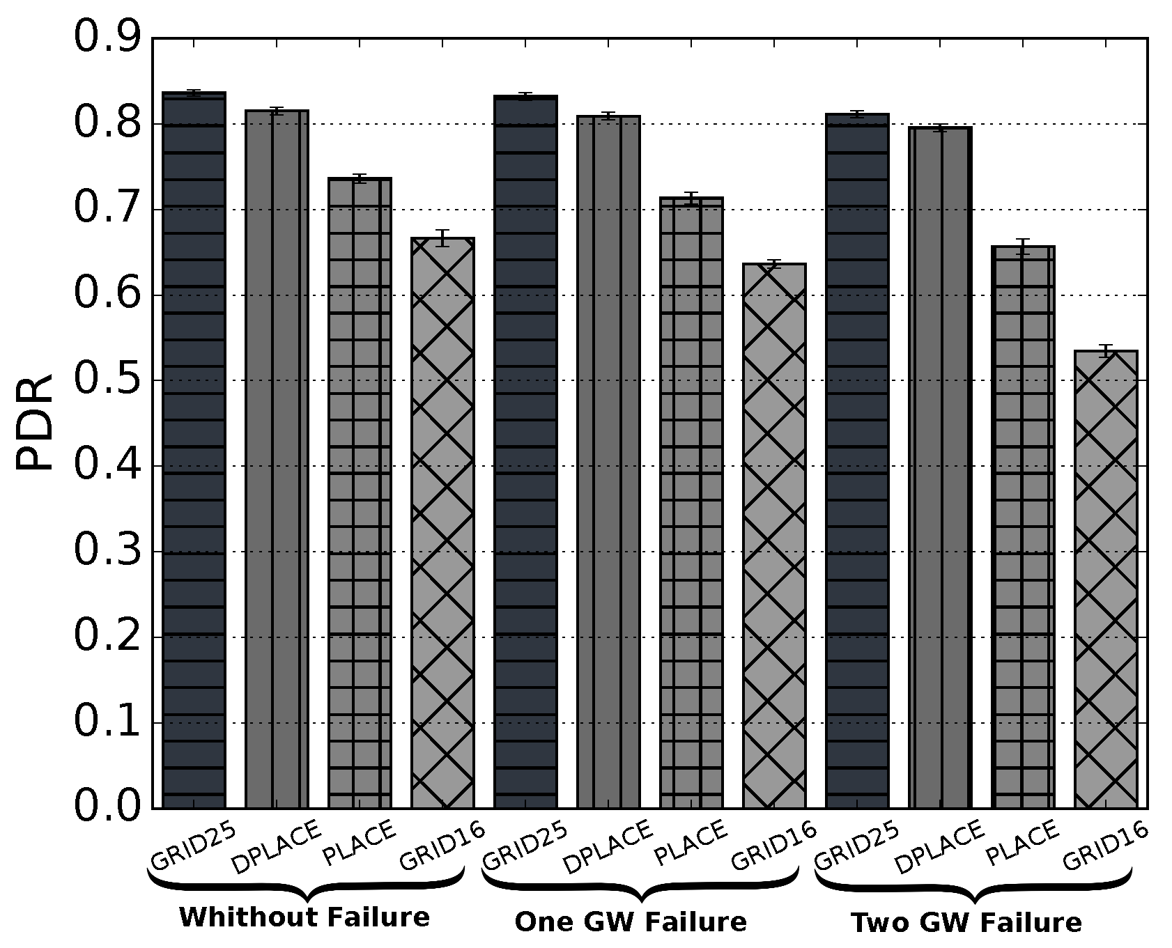
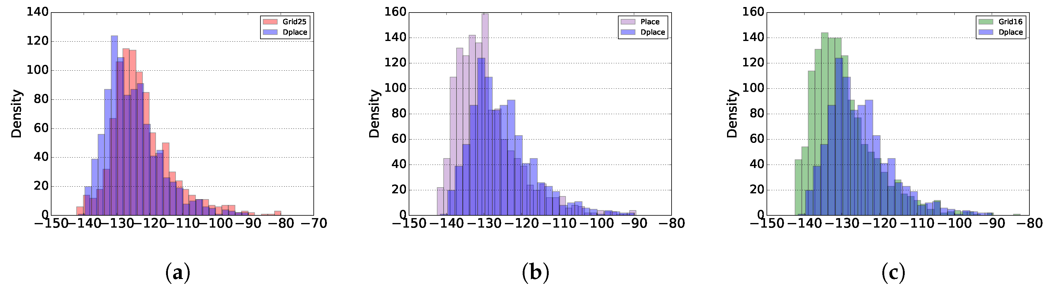
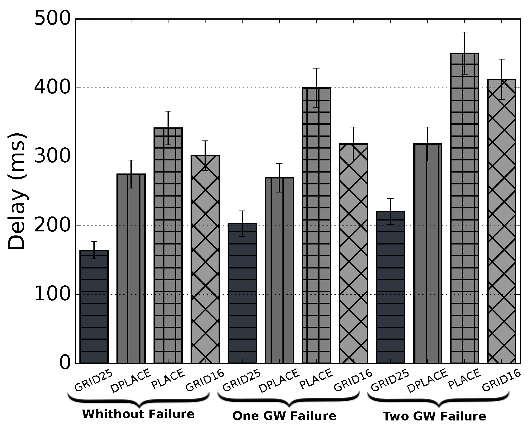
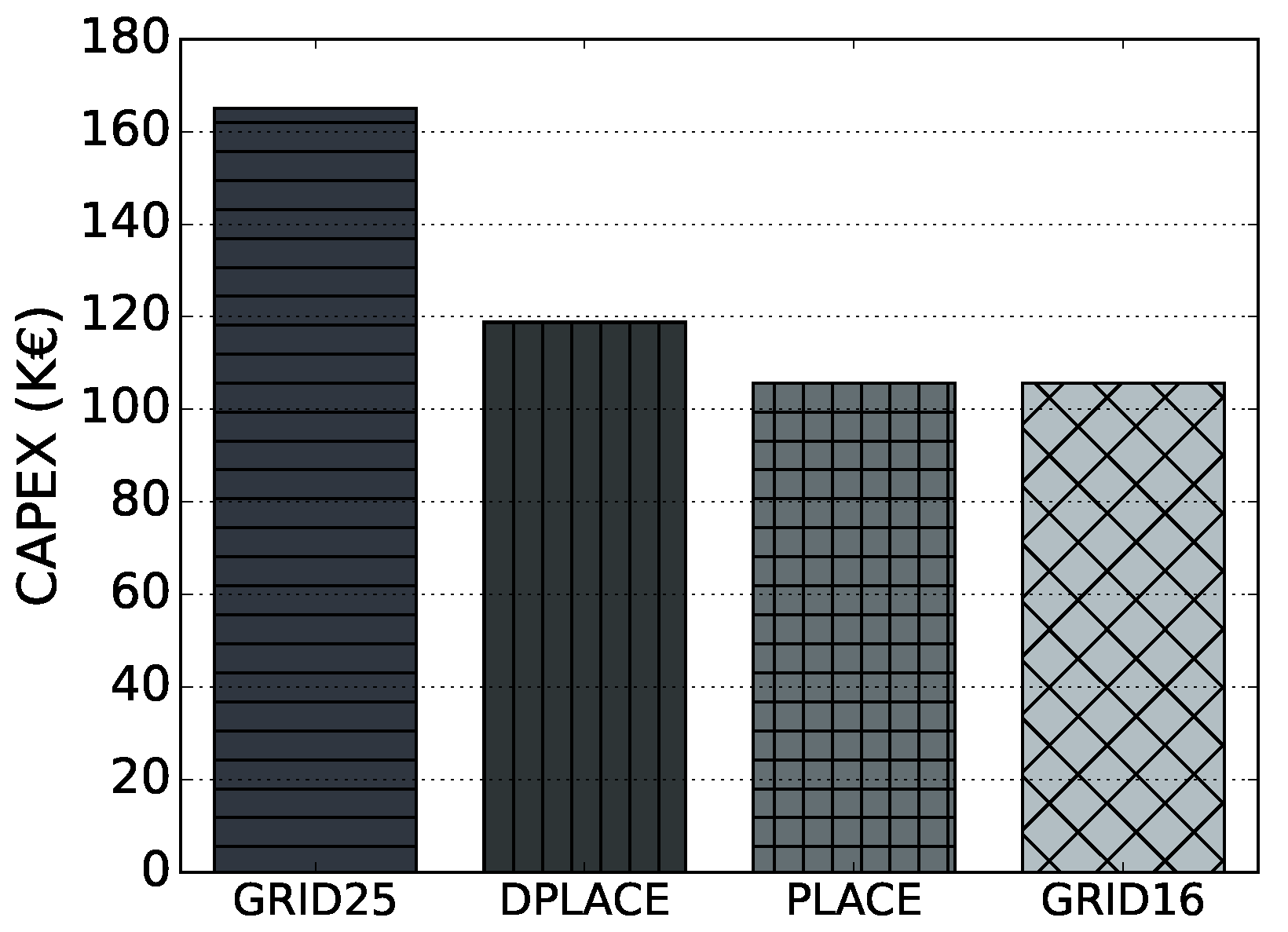
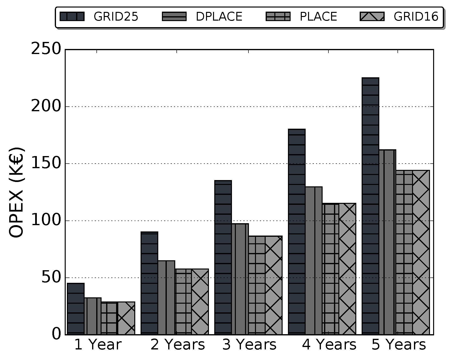
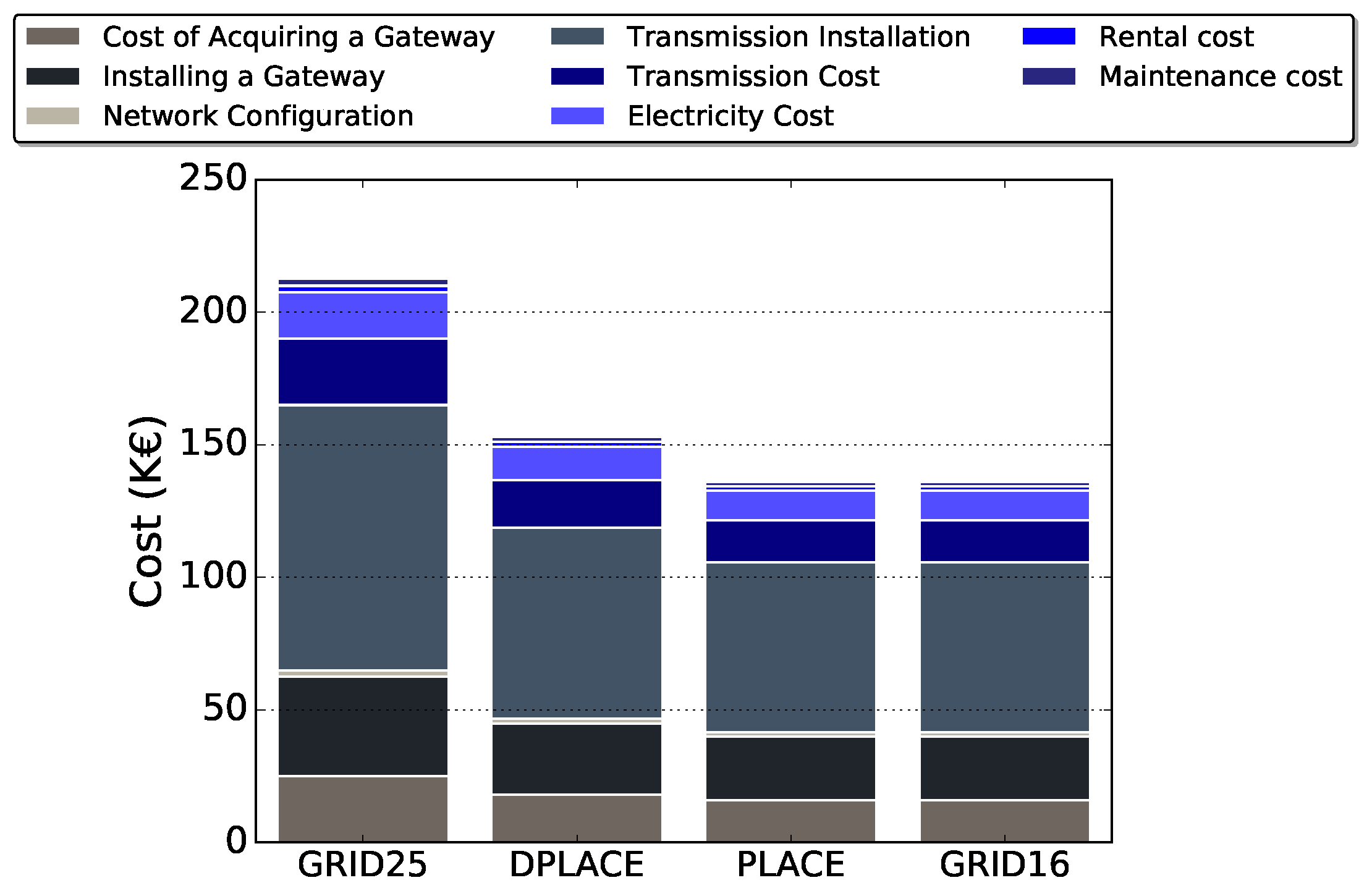
4.2. Results
5. Conclusions
Author Contributions
Funding
Conflicts of Interest
References
- Akpakwu, G.A.; Silva, B.J.; Hancke, G.P.; Abu-Mahfouz, A.M. A survey on 5G networks for the Internet of Things: Communication technologies and challenges. IEEE Access 2018, 6, 3619–3647. [Google Scholar] [CrossRef]
- Ahmadi, H.; Arji, G.; Shahmoradi, L.; Safdari, R.; Nilashi, M.; Alizadeh, M. The application of internet of things in healthcare: A systematic literature review and classification. Univers. Access Inf. Soc. 2018, 18, 837–869. [Google Scholar] [CrossRef]
- Faheem, M.; Shah, S.; Butt, R.; Raza, B.; Anwar, M.; Ashraf, M.; Ngadi, M.A.; Gungor, V. Smart grid communication and information technologies in the perspective of Industry 4.0: Opportunities and challenges. Comput. Sci. Rev. 2018, 30, 1–30. [Google Scholar] [CrossRef]
- Pasolini, G.; Buratti, C.; Feltrin, L.; Zabini, F.; De Castro, C.; Verdone, R.; Andrisano, O. Smart city pilot projects using LoRa and IEEE802. 15.4 technologies. Sensors 2018, 18, 1118. [Google Scholar] [CrossRef] [PubMed]
- Van Der Meulen, R. Gartner Says 6.4 Billion Connected ’Things’ will be in Use in 2016, up 30 Percent from 2015. 2015. Available online: https://www.gartner.com/newsroom/id/3165317(2018/01/15) (accessed on 2 May 2020).
- Cerwall, P.; Jonsson, P.; Möller, R.; Bävertoft, S.; Carson, S.; Godor, I. Ericsson mobility report. In On the Pulse of the Networked Society. Hg. v. Ericsson; Ericsson: Melbourne, Australia, 2015. [Google Scholar]
- Tran, C.; Misra, S. The Technical Foundations of IoT. IEEE Wirel. Commun. 2019, 26, 8. [Google Scholar] [CrossRef]
- Bockelmann, C.; Pratas, N.; Nikopour, H.; Au, K.; Svensson, T.; Stefanovic, C.; Popovski, P.; Dekorsy, A. Massive machine-type communications in 5g: Physical and MAC-layer solutions. IEEE Commun. Mag. 2016, 54, 59–65. [Google Scholar] [CrossRef]
- Adelantado, F.; Vilajosana, X.; Tuset-Peiro, P.; Martinez, B.; Melia-Segui, J.; Watteyne, T. Understanding the Limits of LoRaWAN. IEEE Commun. Mag. 2017, 55, 34–40. [Google Scholar] [CrossRef]
- Mekki, K.; Bajic, E.; Chaxel, F.; Meyer, F. A comparative study of LPWAN technologies for large-scale IoT deployment. ICT Express 2018, 5, 1–7. [Google Scholar] [CrossRef]
- Vejlgaard, B.; Lauridsen, M.; Nguyen, H.; Kovács, I.Z.; Mogensen, P.; Sorensen, M. Interference impact on coverage and capacity for low power wide area IoT networks. In Proceedings of the IEEE Wireless Communications and Networking Conference (WCNC 2017), San Francisco, CA, USA, 19–22 March 2017; pp. 1–6. [Google Scholar]
- Yegin, A.; Kramp, T.; Dufour, P.; Gupta, R.; Soss, R.; Hersent, O.; Hunt, D.; Sornin, N. LoRaWAN protocol: Specifications, security, and capabilities. In LPWAN Technologies for IoT and M2M Applications; Elsevier: Amsterdam, The Netherlands, 2020; pp. 37–63. [Google Scholar]
- Haxhibeqiri, J.; De Poorter, E.; Moerman, I.; Hoebeke, J. A survey of lorawan for IoT: From technology to application. Sensors 2018, 18, 3995. [Google Scholar] [CrossRef] [PubMed]
- Raza, U.; Kulkarni, P.; Sooriyabandara, M. Low power wide area networks: An overview. IEEE Commun. Surv. Tutorials 2017, 19, 855–873. [Google Scholar] [CrossRef]
- Qadir, Q.M.; Rashid, T.A.; Al-Salihi, N.K.; Ismael, B.; Kist, A.A.; Zhang, Z. Low Power Wide Area Networks: A Survey of Enabling Technologies, Applications and Interoperability Needs. IEEE Access 2018, 6, 77454–77473. [Google Scholar] [CrossRef]
- Metzger, F.; Hoßfeld, T.; Bauer, A.; Kounev, S.; Heegaard, P.E. Modeling of aggregated IoT traffic and its application to an IoT cloud. Proc. IEEE 2019, 107, 679–694. [Google Scholar] [CrossRef]
- Petrić, T.; Goessens, M.; Nuaymi, L.; Toutain, L.; Pelov, A. Measurements, performance and analysis of LoRa FABIAN, a real-world implementation of LPWAN. In Proceedings of the IEEE 27th Annual International Symposium on Personal, Indoor, and Mobile Radio Communications (PIMRC 2016), Valencia, Spain, 4–7 September 2016; pp. 1–7. [Google Scholar]
- Wixted, A.J.; Kinnaird, P.; Larijani, H.; Tait, A.; Ahmadinia, A.; Strachan, N. Evaluation of LoRa and LoRaWAN for wireless sensor networks. In Proceedings of the IEEE SENSORS 2016, Orlando, FL, USA, 30 October–3 November 2016; pp. 1–3. [Google Scholar]
- Sanchez-Iborra, R.; Sanchez-Gomez, J.; Ballesta-Viñas, J.; Cano, M.D.; Skarmeta, A. Performance evaluation of LoRa considering scenario conditions. Sensors 2018, 18, 772. [Google Scholar] [CrossRef] [PubMed]
- Tian, H.; Weitnauer, M.; Nyengele, G. Optimized Gateway Placement for Interference Cancellation in Transmit-Only LPWA Networks. Sensors 2018, 18, 3884. [Google Scholar] [CrossRef] [PubMed]
- Gravalos, I.; Makris, P.; Christodoulopoulos, K.; Varvarigos, E.A. Efficient gateways placement for Internet of Things with QoS constraints. In Proceedings of the IEEE Global Communications Conference (GLOBECOM 2016), Washington, DC, USA, 4–8 December 2016; pp. 1–6. [Google Scholar]
- Rady, M.; Hafeez, M.; Zaidi, S.A.R. Computational Methods for Network-Aware and Network-Agnostic IoT Low Power Wide Area Networks (LPWAN). IEEE Internet Things J. 2019, 6, 5732–5744. [Google Scholar] [CrossRef]
- Ousat, B.; Ghaderi, M. LoRa Network Planning: Gateway Placement and Device Configuration. In Proceedings of the IEEE International Congress on Internet of Things (ICIOT 2019), San Diego, CA, USA, 8–13 July 2019; pp. 25–32. [Google Scholar]
- Matni, N.; Moraes, J.; Rosário, D.; Cerqueira, E.; Neto, A. Optimal Gateway Placement Based on Fuzzy C-Means for Low Power Wide Area Networks. In Proceedings of the IEEE Latin-American Conference on Communications (LATINCOM 2019), Salvador, Brazil, 11–13 November 2019; pp. 1–6. [Google Scholar]
- Hossain, M.I.; Lin, L.; Markendahl, J. A Comparative Study of IoT-Communication Systems Cost Structure: Initial Findings of Radio Access Networks Cost. In Proceedings of the 11th CMI International Conference: Prospects and Challenges Towards Developing a Digital Economy within the EU 2018, Copenhagen, Denmark, 29–30 November 2018; pp. 49–55. [Google Scholar]
- Takahashi, R.; Ota, M.; Fukazawa, Y. Fault-Tolerant Topology Determination for IoT Network. In Proceedings of the International Conference on Ubiquitous Information Management and Communication 2019, Phuket, Thailand, 4–6 January 2019; pp. 62–76. [Google Scholar]
- Kumbhar, A.; Koohifar, F.; Güvenç, İ.; Mueller, B. A Survey on Legacy and Emerging Technologies for Public Safety Communications. IEEE Commun. Surv. Tutor. 2017, 19, 97–124. [Google Scholar] [CrossRef]
- Tibshirani, R.; Walther, G.; Hastie, T. Estimating the number of clusters in a data set via the gap statistic. J. R. Stat. Soc. Ser. B 2001, 63, 411–423. [Google Scholar] [CrossRef]
- SX1276, L. 77/78/79 Datasheet. 2019. Available online: Http://www.semtech.com/images/datasheet/sx1276.pdf (accessed on 5 May 2020).
- Van den Abeele, F.; Haxhibeqiri, J.; Moerman, I.; Hoebeke, J. Scalability analysis of large-scale LoRaWAN networks in ns-3. IEEE Internet Things J. 2017, 4, 2186–2198. [Google Scholar] [CrossRef]
- Pop, A.I.; Raza, U.; Kulkarni, P.; Sooriyabandara, M. Does bidirectional traffic do more harm than good in LoRaWAN based LPWA networks? In Proceedings of the GLOBECOM 2017—2017 IEEE Global Communications Conference, Singapore, 4–8 December 2017; pp. 1–6. [Google Scholar]
- Sorensen, R.B.; Razmi, N.; Nielsen, J.J.; Popovski, P. Analysis of LoRaWAN uplink with multiple demodulating paths and capture effect. In Proceedings of the IEEE International Conference on Communications (ICC), Shanghai, China, 20–24 May 2019; pp. 1–6. [Google Scholar]
- Bankov, D.; Khorov, E.; Lyakhov, A. LoRaWAN Modeling and MCS Allocation to Satisfy Heterogeneous QoS Requirements. Sensors 2019, 19, 4204. [Google Scholar] [CrossRef] [PubMed]


| Works | Strategy | Gateway Placement Requirements | |||
|---|---|---|---|---|---|
| Dynamism | Reliability | QoS | Cost | ||
| Tian et al. [20] | Greedy Algorithms | × | ✓ | ✓ | × |
| Gravalos et al. [21] | ILP | × | × | ✓ | ✓ |
| Rady et al. [22] | Machine-Learning | ✓ | × | ✓ | ✓ |
| Ousat and Ghaderi [23] | MINLP | × | × | ✓ | ✓ |
| Matni et al. [24] | Machine-Learning | × | × | ✓ | ✓ |
| Hossain et al. [25] | Deployment Framework | × | × | × | ✓ |
| Symbol | Description |
|---|---|
| M | The maximum number of gateways |
| j | Gateway index () |
| Geographical coordinates of a given gateway j | |
| N | The maximum number of IoT devices |
| i | IoT device index () |
| Geographical coordinates of a given IoT device i | |
| Fuzzy C-Means objective function | |
| The membership coefficient | |
| m | Weighting parameter |
| Euclidean distance between and | |
| B | Number of disorganized data sets |
| b | A disorganized data set index, where, () |
| r | The C-partition matrix inde× |
| C-partition matrix with all the devices membership | |
| K | Number of gateways in Processing phase |
| k | Centroid gateway index in processing phase, where, () |
| Centroid gateway geographical coordinates computed in processing phase |
| SF | sf | sf | sf | sf | sf | sf |
|---|---|---|---|---|---|---|
| Sensitivity | −125 | −128 | −131 | −134 | −136 | 137 |
© 2020 by the authors. Licensee MDPI, Basel, Switzerland. This article is an open access article distributed under the terms and conditions of the Creative Commons Attribution (CC BY) license (http://creativecommons.org/licenses/by/4.0/).
Share and Cite
Matni, N.; Moraes, J.; Oliveira, H.; Rosário, D.; Cerqueira, E. LoRaWAN Gateway Placement Model for Dynamic Internet of Things Scenarios. Sensors 2020, 20, 4336. https://doi.org/10.3390/s20154336
Matni N, Moraes J, Oliveira H, Rosário D, Cerqueira E. LoRaWAN Gateway Placement Model for Dynamic Internet of Things Scenarios. Sensors. 2020; 20(15):4336. https://doi.org/10.3390/s20154336
Chicago/Turabian StyleMatni, Nagib, Jean Moraes, Helder Oliveira, Denis Rosário, and Eduardo Cerqueira. 2020. "LoRaWAN Gateway Placement Model for Dynamic Internet of Things Scenarios" Sensors 20, no. 15: 4336. https://doi.org/10.3390/s20154336
APA StyleMatni, N., Moraes, J., Oliveira, H., Rosário, D., & Cerqueira, E. (2020). LoRaWAN Gateway Placement Model for Dynamic Internet of Things Scenarios. Sensors, 20(15), 4336. https://doi.org/10.3390/s20154336