A Deep Learning Model for Fault Diagnosis with a Deep Neural Network and Feature Fusion on Multi-Channel Sensory Signals


Abstract
1. Introduction
- (1)
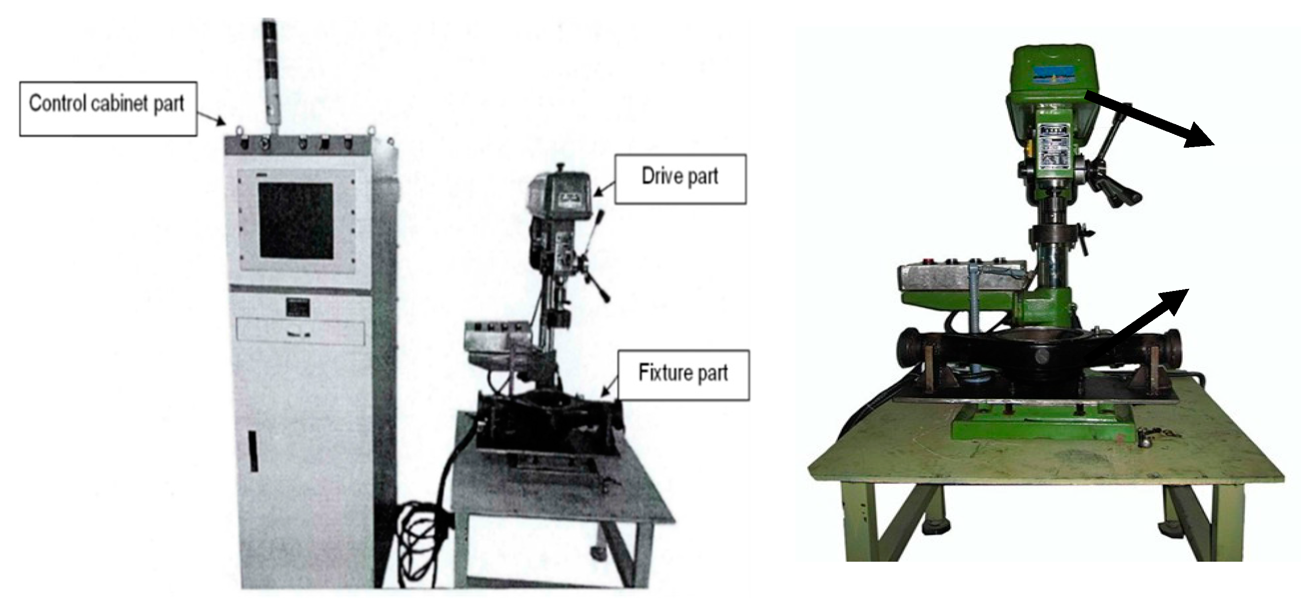
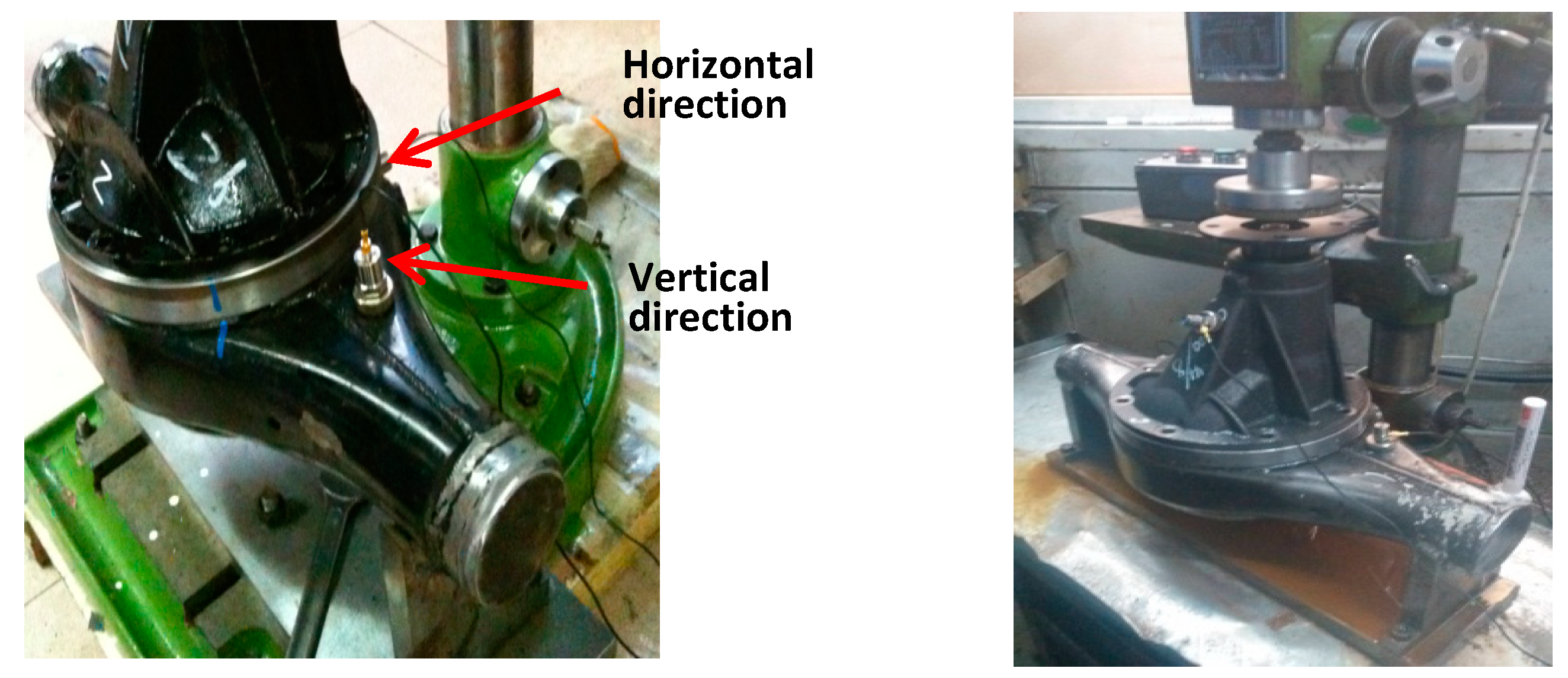
- To solve the limitation of single sensor, we collect multi-channel sensory signals by installing several sensors in different positions along horizontal and vertical direction so as to implement reliable monitoring.
- (2)
- To solve the limitation of using traditional signal process techniques to manually extract features, we employ deep learning technique in learning representative features from original multi-channel signal adaptively.
- (3)
- In order to avoid the heterogeneity and redundancy of deep features from multi-channel data, we fuse these deep features by using locality preserving projection.
2. The Fundamental Theory of Auto-Encoder
3. Proposed Diagnostic Model
3.1. Construction of Deep Neural Network for Deep Feature Learning
3.2. Fusion of Deep Features Extracted from Multi-Channel Signal
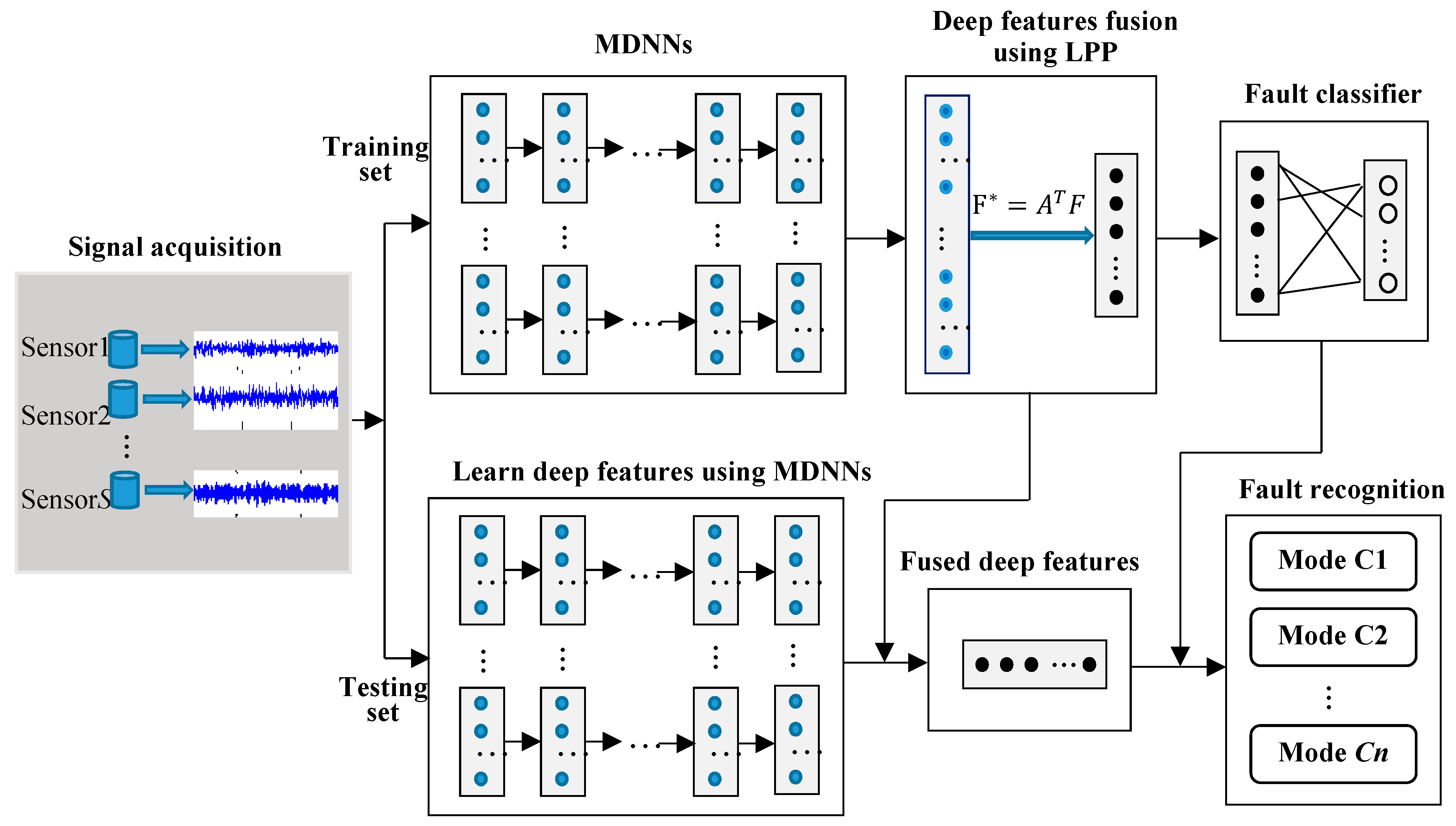
3.3. The Procedure of Intelligent Diagnostic Model
- Step 1:
- Collect multi-channel sensory data from multiple sensors installed in different directions and positions.
- Step 2:
- Without manually extracting features by using traditional signal process techniques, raw data is split up into training subset and testing subset.
- Step 3:
- Construct deep architecture with multiple DNNs to learn fault-sensitive and representative features adaptively from multi-channel sensory signals.
- Step 4:
- Fuse the deep features learned from MDNNs constructed in Step 3 by using LPP, and acquire the representative low-dimensional features.
- Step 5:
- Feed the fused features obtained in Step 4 into the fault classifier based on softmax.
- Step 6:
- Implement fault recognition on the testing set to verify the classification ability and generalization of the method.
4. Experiments and Discussion
4.1. Experimental Arrangement
4.2. Models Design
4.3. Contrast Analysis and Discussion
4.3.1. Validity of the Fusion Strategy
4.3.2. Validity of the Deep Architecture
4.3.3. Representative of Deep Features
4.3.4. Contrastive Analysis and Discussion
- (1)
- In general, deep architecture of neural networks can effectively extract essential and useful features from raw data. However, it is hardly to obtain favorable results by using BPNN with deep architecture. Furthermore, as shown in Table 3, the variance of testing accuracy and training accuracy is obviously higher than other models. It indicates that the performance of BPNN is unstable due to the local minimum problem. The reason for this disadvantage is that the stability of BPNN will be affected by the initial value of network parameters [10]. It may also lead to obvious deviation in the procedure of error back propagation.
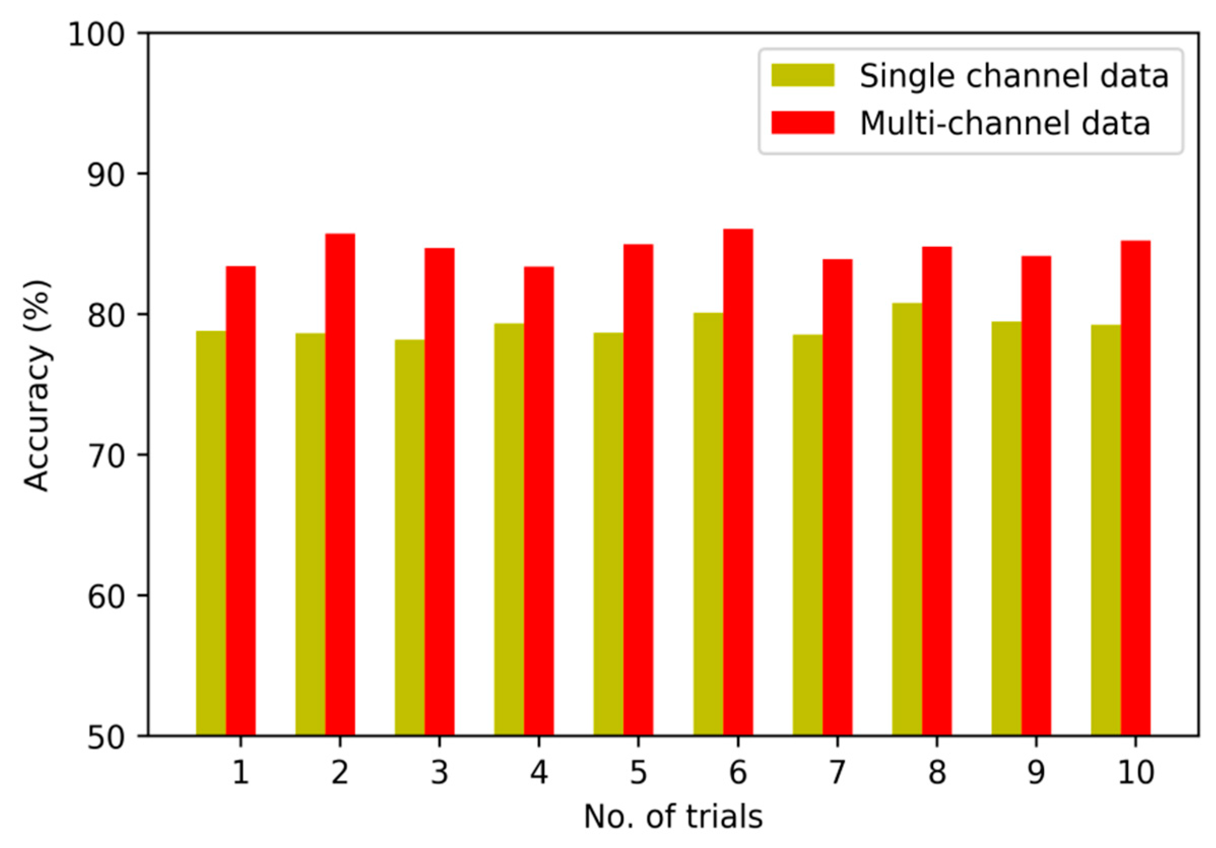
- (2)
- From Table 3, it shows that the deep learning method shows its obvious superiority in feature learning. However, even with multiple hidden layers and multi-channel data, the diagnostic performance of the model based on BPNN is still far from satisfactory, which are 84.56% and 81.14%. Feature learning with deep architecture contains a process of pre-training and a process of fine-tuning. The local minimum problem of traditional BPNN can be obviously solved through the optimization of initial weights layer-by-layer during the procedure of pre-training in unsupervised way and the adjustment of weights during the procedure of fine-tuning in supervised way, which are the typical characteristics of deep neural networks [49].
- (3)
- From the separation of typical features fused from the hidden layers shown in Figure 14, Figure 15 and Figure 16, we can find that a diagnostic model based on MDNNs can automatically extract fault-sensitive features that directly affect the final diagnostic results. In addition, it can adaptively mine the complex non-linear relevance between raw data and several fault modes, which are crucial for condition monitoring [29]. The capability of the model is independent on engineering experiences and prior knowledge in application area.
5. Conclusions
Author Contributions
Funding
Acknowledgments
Conflicts of Interest
References
- Fang, H.-W.; Ma, J. Analysis of transformation countermeasures of automobile manufacturing enterprises from production type to service type. J. Chang’an Univ. (Nat. Sci. Ed.) 2013, 33, 131–136. [Google Scholar]
- Yao, L.-J.; Ding, J.-X. An On-line Vibration Monitoring System for Final Drive of Automobile. Noise Vib. Control 2017, 27, 54–57. [Google Scholar]
- Ye, Q.; Liu, C.; Pan, H. Simultaneous Fault Diagnosis Method Based on Improved Sparse Bayesian Extreme Learning Machine. J. Southwest Jiaotong Univ. 2016, 51, 793–799. [Google Scholar]
- Khazaee, M.; Ahmadi, H.; Omid, M.; Moosavian, A.; Khazaee, M. Classifier fusion of vibration and acoustic signals for fault diagnosis and classification of planetary gears based on Dempster–Shafer evidence theory. Proc. Inst. Mech. Eng. Part E J. Process. Mech. Eng. 2013, 228, 21–32. [Google Scholar] [CrossRef]
- Zhao, R.; Yan, R.; Wang, J.; Mao, K. Learning to Monitor Machine Health with Convolutional Bi-Directional LSTM Networks. Sensors 2017, 17, 273. [Google Scholar] [CrossRef] [PubMed]
- Liu, X.; Tian, Y.; Lei, X.; Liu, M.; Wen, X.; Huang, H.; Wang, H. Deep forest based intelligent fault diagnosis of hydraulic turbine. J. Mech. Sci. Technol. 2019, 33, 2049–2058. [Google Scholar] [CrossRef]
- Lu, Y.; Tang, J.; Luo, H. Wind Turbine Gearbox Fault Detection Using Multiple Sensors With Features Level Data Fusion. J. Eng. Gas Turbines Power 2012, 134, 042501. [Google Scholar] [CrossRef]
- Eren, L.; Ince, T.; Kiranyaz, S. A Generic Intelligent Bearing Fault Diagnosis System Using Compact Adaptive 1D CNN Classifier. J. Signal Process. Syst. 2018, 91, 179–189. [Google Scholar] [CrossRef]
- Yang, Z.; Wong, P.K.; Vong, C.-M.; Zhong, J.; Liang, J. Simultaneous-Fault Diagnosis of Gas Turbine Generator Systems Using a Pairwise-Coupled Probabilistic Classifier. Math. Probl. Eng. 2013, 2013, 1–14. [Google Scholar] [CrossRef]
- Guoji, S.; McLaughlin, S.; Yongcheng, X.; White, P. Theoretical and experimental analysis of bispectrum of vibration signals for fault diagnosis of gears. Mech. Syst. Signal Process. 2014, 43, 76–89. [Google Scholar] [CrossRef]
- Jena, D.; Sahoo, S.; Panigrahi, S. Gear fault diagnosis using active noise cancellation and adaptive wavelet transform. Measurement 2014, 47, 356–372. [Google Scholar] [CrossRef]
- Amarnath, M.; Krishna, I.P. Local fault detection in helical gears via vibration and acoustic signals using EMD based statistical parameter analysis. Measurement 2014, 58, 154–164. [Google Scholar] [CrossRef]
- Ye, Q.; Liu, C. A Multichannel Data Fusion Method Based on Multiple Deep Belief Networks for Intelligent Fault Diagnosis of Main Reducer. Symmetry 2020, 12, 483. [Google Scholar] [CrossRef]
- Zhou, C.; Zhou, J.-F. Direction-of-Arrival Estimation with Coarray ESPRIT for Coprime Array. Sensors 2017, 17, 1779. [Google Scholar] [CrossRef]
- Wen, F.; Shi, J. Fast direction finding for bistatic EMVS-MIMO radar without pairing. Signal Process. 2020, 173, 107512. [Google Scholar] [CrossRef]
- Zhou, C.; Gu, Y.; Fan, X.; Shi, Z.; Mao, G.; Zhang, Y.D. Direction-of-Arrival Estimation for Coprime Array via Virtual Array Interpolation. IEEE Trans. Signal Process. 2018, 66, 5956–5971. [Google Scholar] [CrossRef]
- Liu, T.; Wen, F.; Zhang, L.; Wang, K. Off-Grid DOA Estimation for Colocated MIMO Radar via Reduced-Complexity Sparse Bayesian Learning. IEEE Access 2019, 7, 99907–99916. [Google Scholar] [CrossRef]
- Zhou, C.; Gu, Y.; He, S.; Shi, Z. A Robust and Efficient Algorithm for Coprime Array Adaptive Beamforming. IEEE Trans. Veh. Technol. 2018, 67, 1099–1112. [Google Scholar] [CrossRef]
- Wen, F.; Zhang, Z.; Wang, K.; Sheng, G.; Zhang, G. Angle estimation and mutual coupling self-calibration for ULA-based bistatic MIMO radar. Signal Process. 2018, 144, 61–67. [Google Scholar] [CrossRef]
- Zhou, C.; Gu, Y.; Zhang, Y.D.; Shi, Z.; Jin, T.; Wu, X. Compressive sensing-based coprime array direction-of-arrival estimation. IET Commun. 2017, 11, 1719–1724. [Google Scholar] [CrossRef]
- Shi, Z.; Zhou, C.; Gu, Y.; Goodman, N.A.; Qu, F. Source Estimation Using Coprime Array: A Sparse Reconstruction Perspective. IEEE Sens. J. 2017, 17, 755–765. [Google Scholar] [CrossRef]
- Song, J.; Liu, Y.; Shao, J.; Tang, C. A Dynamic Membership Data Aggregation (DMDA) Protocol for Smart Grid. IEEE Syst. J. 2020, 14, 900–908. [Google Scholar] [CrossRef]
- Vanra, J.; Dhami, S.S.; Pabla, B. Hybrid data fusion approach for fault diagnosis of fixed-axis gearbox. Struct. Health Monit. 2017, 17, 936–945. [Google Scholar] [CrossRef]
- Li, C.; Sánchez, R.-V.; Zurita, G.; Cerrada, M.; Cabrera, D.; Vásquez, R.E. Gearbox fault diagnosis based on deep random forest fusion of acoustic and vibratory signals. Mech. Syst. Signal Process. 2016, 76, 283–293. [Google Scholar] [CrossRef]
- Nembhard, A.D.; Sinha, J.K.; Yunusa-Kaltungo, A. Development of a generic rotating machinery fault diagnosis approach insensitive to machine speed and support type. J. Sound Vib. 2015, 337, 321–341. [Google Scholar] [CrossRef]
- Yunusa-Kaltungo, A.; Sinha, J.; Nembhard, A.D. A novel fault diagnosis technique for enhancing maintenance and reliability of rotating machines. Struct. Heal. Monit. 2015, 14, 604–621. [Google Scholar] [CrossRef]
- Lei, Y.; Lin, J.; He, Z.; Kong, D. A Method Based on Multi-Sensor Data Fusion for Fault Detection of Planetary Gearboxes. Sensors 2012, 12, 2005–2017. [Google Scholar] [CrossRef]
- Safizadeh, M.; Latifi, S. Using multi-sensor data fusion for vibration fault diagnosis of rolling element bearings by accelerometer and load cell. Inf. Fusion 2014, 18, 1–8. [Google Scholar] [CrossRef]
- Jing, L.; Wang, T.; Zhao, M.; Wang, P. An Adaptive Multi-Sensor Data Fusion Method Based on Deep Convolutional Neural Networks for Fault Diagnosis of Planetary Gearbox. Sensors 2017, 17, 414. [Google Scholar] [CrossRef]
- Li, Z.; Yan, X.; Wang, X.; Peng, Z. Detection of gear cracks in a complex gearbox of wind turbines using supervised bounded component analysis of vibration signals collected from multi-channel sensors. J. Sound Vib. 2016, 371, 406–433. [Google Scholar] [CrossRef]
- Duro, J.A.; Padget, J.; Bowen, C.R.; Kim, H.A.; Nassehi, A. Multi-sensor data fusion framework for CNC machining monitoring. Mech. Syst. Signal Process. 2016, 66, 505–520. [Google Scholar] [CrossRef]
- Khazaee, M.; Ahmadi, H.; Omid, M.; Banakar, A.; Moosavian, A. Feature-level fusion based on wavelet transform and artificial neural network for fault diagnosis of planetary gearbox using acoustic and vibration signals. Insight-Non-Destr. Test. Cond. Monit. 2013, 55, 323–330. [Google Scholar] [CrossRef]
- Yunusa-Kaltungo, A.; Cao, R. Towards Developing an Automated Faults Characterisation Framework for Rotating Machines. Part 1: Rotor-Related Faults. Energies 2020, 13, 1394. [Google Scholar] [CrossRef]
- Liu, Z.; Guo, W.; Tang, Z.-C.; Chen, Y. Multi-Sensor Data Fusion Using a Relevance Vector Machine Based on an Ant Colony for Gearbox Fault Detection. Sensors 2015, 15, 21857–21875. [Google Scholar] [CrossRef]
- Su, Z.; Tang, B.; Liu, Z.; Qin, Y. Multi-fault diagnosis for rotating machinery based on orthogonal supervised linear local tangent space alignment and least square support vector machine. Neurocomputing 2015, 157, 208–222. [Google Scholar] [CrossRef]
- Li, C.; Sánchez, R.-V.; Zurita, G.; Cerrada, M.; Cabrera, D. Fault Diagnosis for Rotating Machinery Using Vibration Measurement Deep Statistical Feature Learning. Sensors 2016, 16, 895. [Google Scholar] [CrossRef]
- Jia, F.; Lei, Y.; Lin, J.; Zhou, X.; Lu, N. Deep neural networks: A promising tool for fault characteristic mining and intelligent diagnosis of rotating machinery with massive data. Mech. Syst. Signal Process. 2016, 72, 303–315. [Google Scholar] [CrossRef]
- LeCun, Y.; Bengio, Y.; Hinton, G. Review: Deep learning. Nature 2015, 521, 436–444. [Google Scholar] [CrossRef]
- Liu, W.; Wang, Z.; Liu, X.; Zeng, N.; Liu, Y.; Alsaadi, F.E. A survey of deep neural network architectures and their applications. Neurocomputing 2017, 234, 11–26. [Google Scholar] [CrossRef]
- Schmidhuber, J. Deep learning in neural networks: An overview. Neural Netw. 2015, 61, 85–117. [Google Scholar] [CrossRef]
- Chandra, B.; Sharma, R.K. Fast learning in Deep Neural Networks. Neurocomputing 2016, 171, 1205–1215. [Google Scholar] [CrossRef]
- Suk, H.-I.; Lee, S.-W.; Shen, D.; Initiative, T.A.D.N. Hierarchical feature representation and multimodal fusion with deep learning for AD/MCI diagnosis. NeuroImage 2014, 101, 569–582. [Google Scholar] [CrossRef] [PubMed]
- Sun, W.; Shao, S.; Zhao, R.; Yan, R.; Zhang, X.; Chen, X. A sparse auto-encoder-based deep neural network approach for induction motor faults classification. Measurement 2016, 89, 171–178. [Google Scholar] [CrossRef]
- Tamilselvan, P.; Wang, P. Failure diagnosis using deep belief learning based health state classification. Reliab. Eng. Syst. Saf. 2013, 115, 124–135. [Google Scholar] [CrossRef]
- Hinton, G.; Mohamed, A.-R.; Jaitly, N.; Vanhoucke, V.; Kingsbury, B.; Deng, L.; Yu, D.; Dahl, G.; Senior, A.W.; Nguyen, P.; et al. Deep Neural Networks for Acoustic Modeling in Speech Recognition: The Shared Views of Four Research Groups. IEEE Signal Process. Mag. 2012, 29, 82–97. [Google Scholar] [CrossRef]
- Shao, H.; Jiang, H.; Zhao, H.; Wang, F. A novel deep autoencoder feature learning method for rotating machinery fault diagnosis. Mech. Syst. Signal Process. 2017, 95, 187–204. [Google Scholar] [CrossRef]
- Zabalza, J.; Ren, J.; Zheng, J.; Zhao, H.; Qing, C.; Yang, Z.; Du, P.; Marshall, S. Novel segmented stacked autoencoder for effective dimensionality reduction and feature extraction in hyperspectral imaging. Neurocomputing 2016, 185, 1–10. [Google Scholar] [CrossRef]
- Xiong, P.; Wang, H.; Liu, M.; Zhou, S.; Hou, Z.; Lin, C. ECG signal enhancement based on improved denoising auto-encoder. Eng. Appl. Artif. Intell. 2016, 52, 194–202. [Google Scholar] [CrossRef]
- Shao, H.; Jiang, H.; Wang, F.; Zhao, H. An enhancement deep feature fusion method for rotating machinery fault diagnosis. Knowl.-Based Syst. 2017, 119, 200–220. [Google Scholar] [CrossRef]
- Shikkenawis, G.; Mitra, S. A New Proposal for Locality Preserving Projection. Comput. Vis. 2012, 7143, 298–305. [Google Scholar]
- Ding, X.; He, Q.; Luo, N. A fusion feature and its improvement based on locality preserving projections for rolling element bearing fault classification. J. Sound Vib. 2015, 335, 367–383. [Google Scholar] [CrossRef]
- Fan, Q.; Gao, D.Q.; Wang, Z. Multiple empirical kernel learning with locality pre-serving constraint. Knowl.-Based Syst. 2016, 105, 107–118. [Google Scholar] [CrossRef]
- Chen, L.; Zhou, M.; Su, W.; Wu, M.; She, J.; Hirota, K. Softmax regression based deep sparse autoencoder network for facial emotion recognition in human-robot interaction. Inf. Sci. 2018, 428, 49–61. [Google Scholar] [CrossRef]
- Du, J.; Xu, Y. Hierarchical deep neural network for multivariate regression. Pattern Recognit. 2017, 63, 149–157. [Google Scholar] [CrossRef]
- Guo, X.; Chen, L.; Shen, C. Hierarchical adaptive deep convolution neural network and its application to bearing fault diagnosis. Measurement 2016, 93, 490–502. [Google Scholar] [CrossRef]
- Lu, C.; Wang, Z.-Y.; Qin, W.-L.; Ma, J. Fault diagnosis of rotary machinery components using a stacked denoising autoencoder-based health state identification. Signal Process. 2017, 130, 377–388. [Google Scholar] [CrossRef]
- Shin, H.-C.; Orton, M.R.; Collins, D.J.; Doran, S.J.; Leach, M.O. Stacked Autoencoders for Unsupervised Feature Learning and Multiple Organ Detection in a Pilot Study Using 4D Patient Data. IEEE Trans. Pattern Anal. Mach. Intell. 2013, 35, 1930–1943. [Google Scholar] [CrossRef]
- Nousi, P.; Tefas, A. Deep learning algorithms for discriminant autoencoding. Neurocomputing 2017, 266, 325–335. [Google Scholar] [CrossRef]
- Galdámez, P.L.; Raveane, W.; Arrieta, A.G. A brief review of the ear recognition process using deep neural networks. J. Appl. Log. 2017, 24, 62–70. [Google Scholar] [CrossRef]
- Yu, D. Bearing performance degradation assessment using locality preserving projections and Gaussian mixture models. Mech. Syst. Signal Process. 2011, 25, 2573–2588. [Google Scholar] [CrossRef]
- Bao, S.; Luo, L.; Mao, J.; Tang, D. Improved fault detection and diagnosis using sparse global-local preserving projections. J. Process. Control. 2016, 47, 121–135. [Google Scholar] [CrossRef]


| Label | Fault Patterns | Size of Training Set | Size of Testing Set |
|---|---|---|---|
| C1 | Normal status | 1400 | 350 |
| C2 | Gear crack | 1400 | 350 |
| C3 | Gear error | 1400 | 350 |
| C4 | Gear tooth broken | 1400 | 350 |
| C5 | Gear burr | 1400 | 350 |
| C6 | Misalignment | 1400 | 350 |
| C7 | Gear hard point | 1400 | 350 |
| Models | Average Testing Accuracy (%) | |
|---|---|---|
| Features Manually Extracted with Signal Pre-Processing | Features Adaptively Extracted without Pre-Processing | |
| The proposed model | 94.23 (1.54) | 93.84 (0.73) |
| Model based on BPNN | 84.27 (3.81) | 81.46 (4.32) |
| Model based on SVM | 79.62 (2.88) | 76.49 (2.92) |
| Models | Average Training Accuracy (%) | Average Testing Accuracy (%) | ||
|---|---|---|---|---|
| Single-Channel Data | Multi-Channel Data | Single-Channel Data | Multi-Channel Data | |
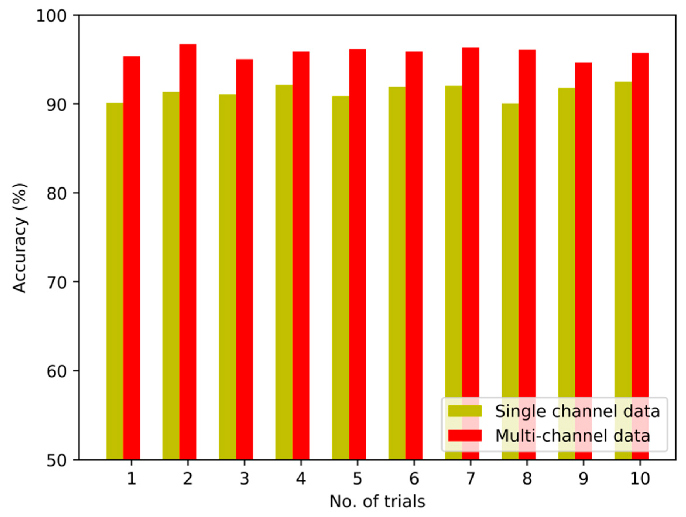
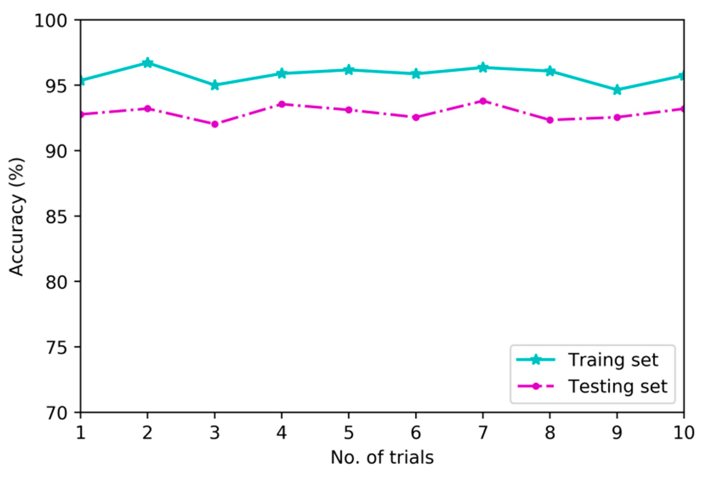
| The proposed method | 91.42 (1.11) | 95.84 (0.94) | 90.17 (1.29) | 92.76 (1.13) |
| Model based on BPNN | 79.09 (4.59) | 84.56 (3.72) | 76.29 (4.80) | 81.14 (4.05) |
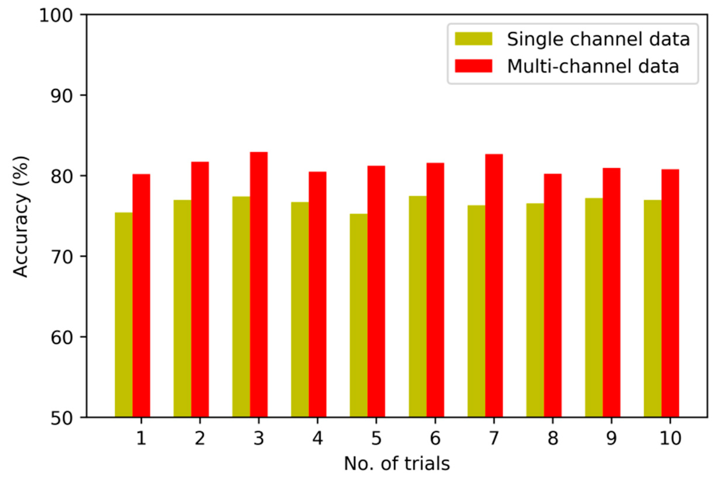
| Model based on SVM | 76.62 (2.97) | 81.28 (2.63) | 74.32 (3.47) | 77.63 (3.06) |
| Models | Average Training Time (s) | |
|---|---|---|
| Without Fusion Multi-Channel Data | Fusion Multi-Channel Data | |
| The proposed model | 58.56 | 39.49 |
| Model based on BPNN | 30.39 | 18.61 |
| Model based on SVM | 10.22 | 5.93 |
© 2020 by the authors. Licensee MDPI, Basel, Switzerland. This article is an open access article distributed under the terms and conditions of the Creative Commons Attribution (CC BY) license (http://creativecommons.org/licenses/by/4.0/).
Share and Cite
Ye, Q.; Liu, S.; Liu, C. A Deep Learning Model for Fault Diagnosis with a Deep Neural Network and Feature Fusion on Multi-Channel Sensory Signals. Sensors 2020, 20, 4300. https://doi.org/10.3390/s20154300
Ye Q, Liu S, Liu C. A Deep Learning Model for Fault Diagnosis with a Deep Neural Network and Feature Fusion on Multi-Channel Sensory Signals. Sensors. 2020; 20(15):4300. https://doi.org/10.3390/s20154300
Chicago/Turabian StyleYe, Qing, Shaohu Liu, and Changhua Liu. 2020. "A Deep Learning Model for Fault Diagnosis with a Deep Neural Network and Feature Fusion on Multi-Channel Sensory Signals" Sensors 20, no. 15: 4300. https://doi.org/10.3390/s20154300
APA StyleYe, Q., Liu, S., & Liu, C. (2020). A Deep Learning Model for Fault Diagnosis with a Deep Neural Network and Feature Fusion on Multi-Channel Sensory Signals. Sensors, 20(15), 4300. https://doi.org/10.3390/s20154300