Gain-Phase Errors Calibration for a Linear Array Based on Blind Signal Separation


Abstract
1. Introduction
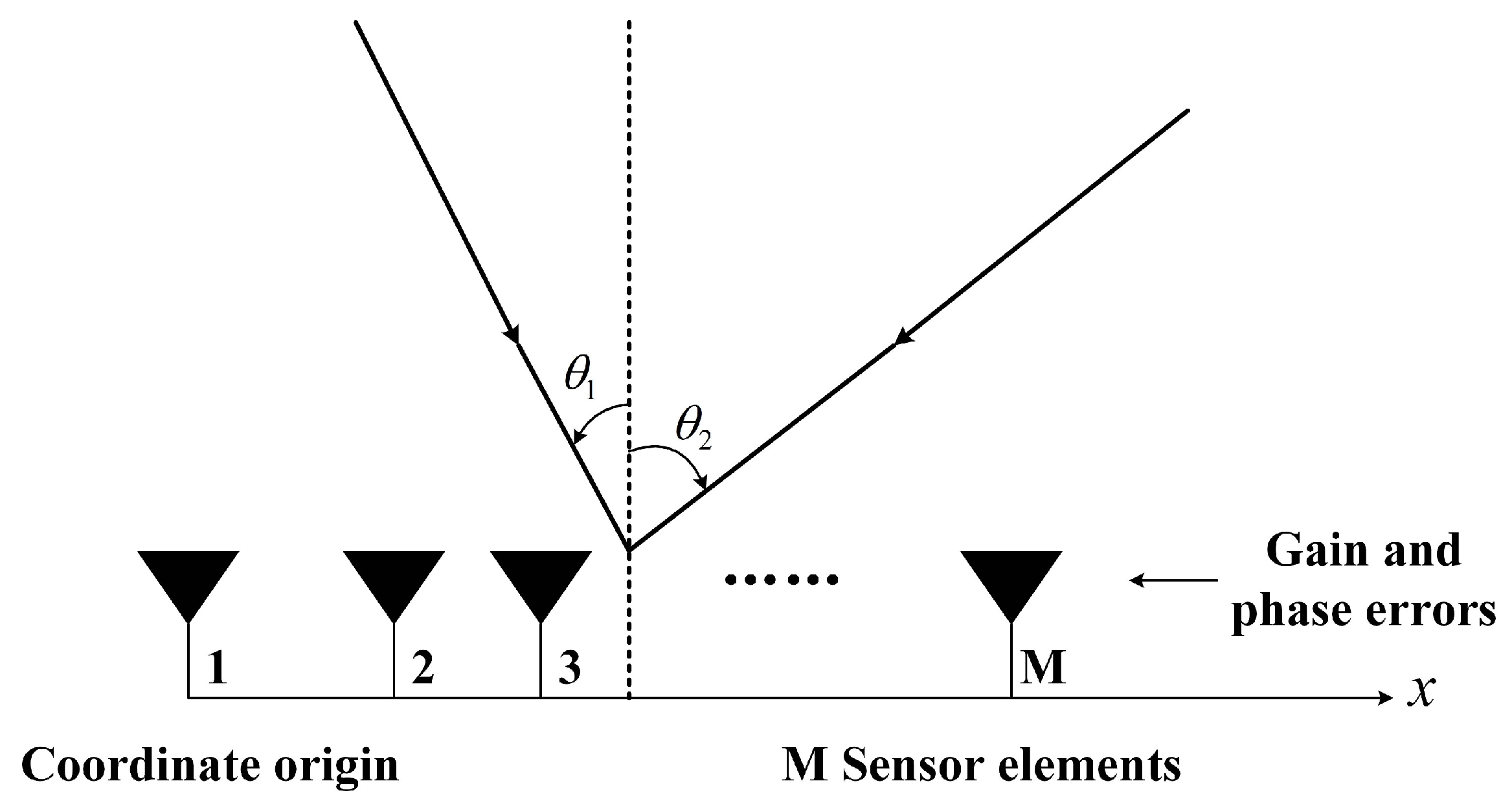
2. Data Model
3. Proposed Algorithm
3.1. Mixing Matrix Estimation
3.2. Doa Estimation
3.3. Gain-Phase Errors Estimation
4. Discussion
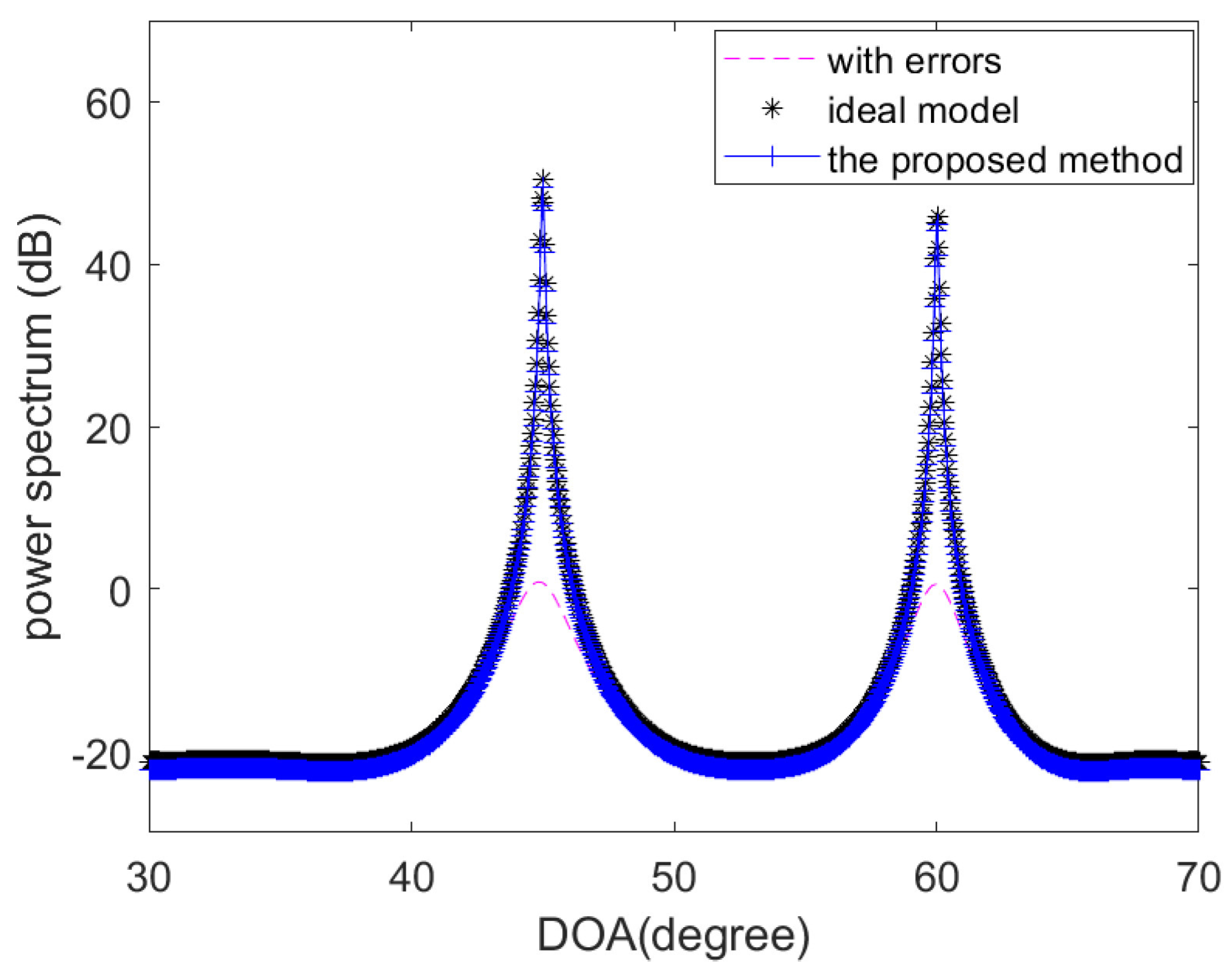
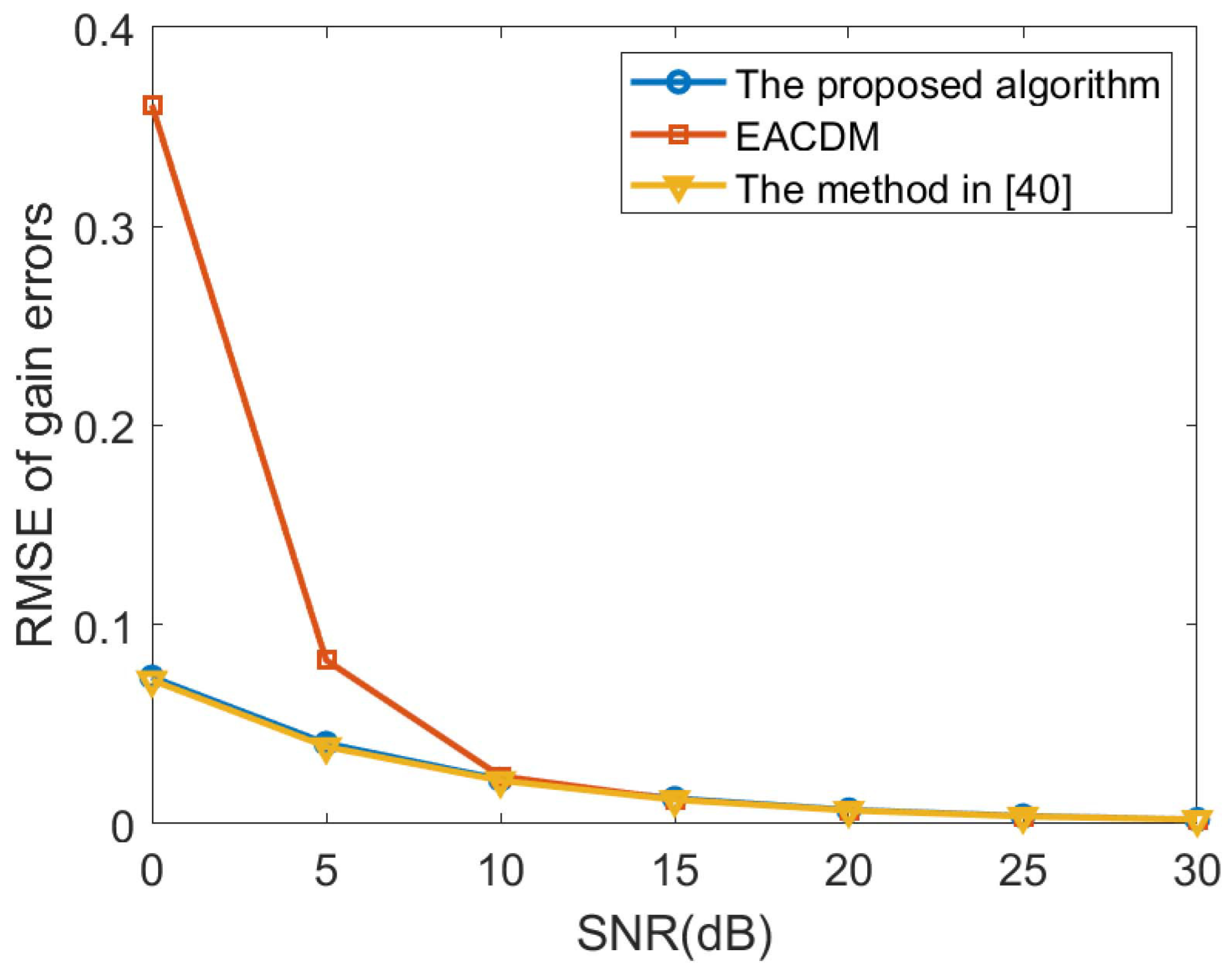
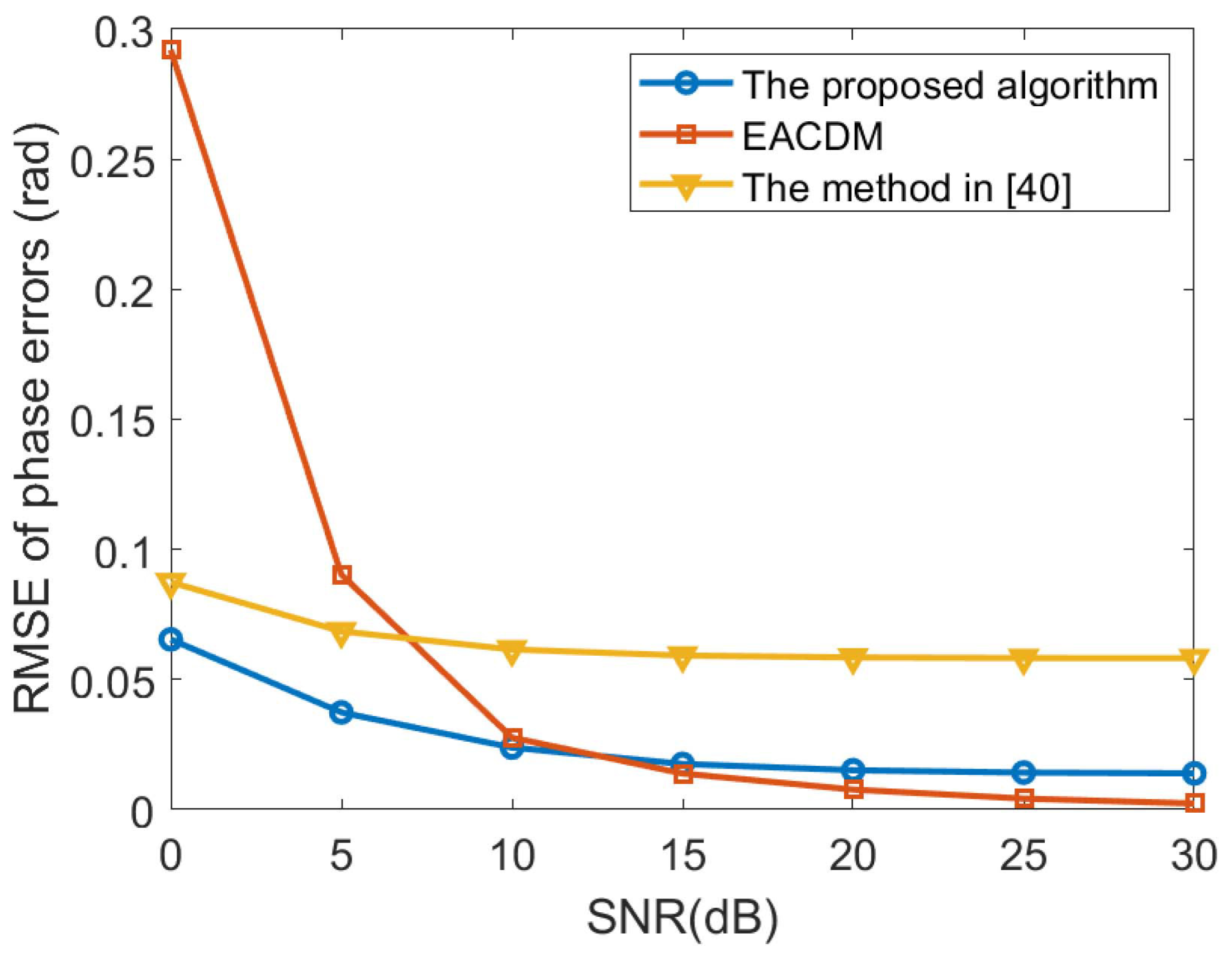
5. Numerical Simulations
6. Conclusions
Author Contributions
Funding
Conflicts of Interest
References
- Zhou, C.; Shi, Z.; Gu, Y.; Shen, X. DECOM: DOA estimation with combined MUSIC for coprime array. In Proceedings of the 2013 International Conference on Wireless Communications and Signal Processing, Hangzhou, China, 24–26 October 2013; pp. 1–5. [Google Scholar]
- Zhou, C.; Zhou, J. Direction-of-Arrival Estimation with Coarray ESPRIT for Coprime Array. Sensors 2017, 17, 1779. [Google Scholar] [CrossRef] [PubMed]
- Shi, Z.; Zhou, C.; Gu, Y.; Goodman, N.; Qu, F. Source estimation using coprime array: A sparse reconstruction perspective. IEEE Sens. J. 2017, 17, 755–765. [Google Scholar] [CrossRef]
- Zhou, C.; Gu, Y.; He, S.; Shi, Z. A Robust and Efficient Algorithm for Coprime Array Adaptive Beamforming. IEEE Trans. Veh. Technol. 2018, 67, 1099–1112. [Google Scholar] [CrossRef]
- Zhou, C.; Gu, Y.; Zhang, Y.; Shi, Z.; Jin, T.; Wu, D. Compressive sensing-based coprime array direction-of-arrival estimation. IET Commun. 2017, 11, 1719–1724. [Google Scholar] [CrossRef]
- Zhou, C.; Gu, Y.; Fang, X.; Shi, Z.; Mao, G.; Zhang, Y. Direction-of-arrival estimation for coprime array via virtual array interpolation. IEEE Trans. Signal Process. 2018, 22, 5956–5971. [Google Scholar] [CrossRef]
- Zhou, C.; Gu, Y.; Shi, Z.; Zhang, Y. Off-grid direction-of-arrival estimation using coprime array interpolation. IEEE Signal Process. Lett. 2018, 11, 1710–1714. [Google Scholar] [CrossRef]
- Wen, F.; Shi, J. Fast direction finding for bistatic EMVS-MIMO radar without pairing. Signal Process. 2020, 173, 1–8. [Google Scholar] [CrossRef]
- Wen, F.; Mao, C.; Zhang, G. Direction finding in MIMO radar with large antenna arrays and nonorthogonal waveforms. Digit. Signal Process. 2019, 94, 75–83. [Google Scholar] [CrossRef]
- Wen, F.; Zhang, Z.; Zhang, G. Joint DOD and DOA estimation for bistatic MIMO radar: A covariance trilinear decomposition perspective. IEEE Access. 2019, 7, 53273–53283. [Google Scholar] [CrossRef]
- Wen, F.; Zhang, Z.; Wang, K.; Sheng, G.; Zhang, G. Angle estimation and mutual coupling self-calibration for ULA-based bistatic MIMO radar. Signal Process. 2018, 144, 61–67. [Google Scholar] [CrossRef]
- Wen, F.; Xiong, X.; Zhang, Z. Angle and mutual coupling estimation in bistatic MIMO radar based on PARAFAC decomposition. Digit. Signal Process. 2017, 65, 1–10. [Google Scholar] [CrossRef]
- Fuhrmann, D.R. Estimation of sensor gain and phase. IEEE Trans. Signal Process. 1994, 1, 77–87. [Google Scholar] [CrossRef]
- Cheng, Q.; Hua, Y.; Stoica, P. Asymptotic performance of optimal gain-and-phase estimators of sensor arrays. IEEE Trans. Signal Process. 2000, 12, 3587–3590. [Google Scholar]
- Ng, B.P.; Lie, J.P.; Er, M.H.; Feng, A. A practical simple geometry and gain/Phase calibration technique for antenna array processing. IEEE Trans. Antennas Propag. 2009, 7, 1963–1972. [Google Scholar]
- Jiang, J.; Duan, F.; Chen, J.; Chao, Z.; Chang, Z.; Hua, X. Two new estimation algorithms for sensor gain and phase errors based on different data models. IEEE Sens. J. 2013, 5, 1921–1930. [Google Scholar] [CrossRef]
- Wang, D.; Ke, K.; Zhang, X.; Wu, Y. Robust calibration algorithm for multiplicative modeling errors against location deviations of auxiliary sources. Circuits, Syst. Signal Process. 2014, 8, 2495–2519. [Google Scholar] [CrossRef]
- Guo, Y.; Zhang, Y.; Tong, N. ESPRIT-like angle estimation for bistatic MIMO radar with gain and phase uncertainties. Electron. Lett. 2011, 17, 996–997. [Google Scholar] [CrossRef]
- Chen, C.; Zhang, X. Joint angle and array gain-phase errors estimation using PM-like algorithm for bistatic MIMO radar. Circuits, Systems, and Signal Process. 2013, 3, 1293–1311. [Google Scholar] [CrossRef]
- Li, J.; Zhang, X.; Gao, X. A joint scheme for angle and array gain-phase error estimation in bistatic MIMO radar. IEEE Geosci. Remote Sensing Lett. 2013, 6, 1478–1482. [Google Scholar] [CrossRef]
- Liao, B.; Chan, S. Direction finding in MIMO radar with unknown transmitter and/or receiver gains and phases. Multidim. Syst. Sign. Process. 2017, 2, 691–707. [Google Scholar] [CrossRef]
- Li, J.; Zhang, X.; Cao, R.; Zhou, M. Reduced-dimension MUSIC for angle and array gain-phase error estimation in bistatic MIMO radar. IEEE Commun. Lett. 2013, 3, 443–446. [Google Scholar] [CrossRef]
- Li, J.; Jin, M.; Zheng, Y.; Liao, G.; Lv, L. Transmit and receive array gain-phase error estimation in bistatic MIMO radar. IEEE Antennas Wirel. Propag. Lett. 2015, 14, 32–35. [Google Scholar] [CrossRef]
- Weiss, A.J.; Friedlander, B. Eigenstructure methods for direction finding with sensor gain and phase uncertainties. Circuits Syst. Signal Process. 1990, 3, 271–300. [Google Scholar] [CrossRef]
- Friedlander, B.; Weiss, A.J. Direction finding in the presence of mutual coupling. IEEE Trans. Antennas Propag. 1991, 3, 273–284. [Google Scholar] [CrossRef]
- Hung, E. A critical study of a self-calibrating direction-finding method for arrays. IEEE Trans. Signal Process. 1994, 2, 471–474. [Google Scholar] [CrossRef]
- Jansson, M.; Swindlehurst, A.L.; Ottersten, B. Weighted subspace fitting for general array error models. IEEE Trans. Signal Process. 1998, 9, 2484–2498. [Google Scholar] [CrossRef]
- Wijnholds, S.J.; Veen, A. Multisource self-calibration for sensor arrays. IEEE Trans. Signal Process. 2009, 9, 3512–3522. [Google Scholar] [CrossRef]
- Hong, J.S. Genetic approach to bearing estimation with sensor location uncertainties. Electron. Lett. 1993, 23, 2013–2014. [Google Scholar] [CrossRef]
- Li, M.; Lu, Y. Source bearing and steering-vector estimation using partially calibrated arrays. IEEE Trans. Aerosp. Electron. Syst. 2009, 4, 1361–1372. [Google Scholar]
- Li, M.; Lu, Y. Maximum likelihood processing for arrays with partially unknown sensor gains and phases. In Proceedings of the International Conference on ITS Telecommunications, Sophia Antipolis, France, 6–8 June 2007; pp. 1–6. [Google Scholar]
- Comon, P. Independent component analysis: A new concept. Signal Process. 1994, 36, 287–314. [Google Scholar] [CrossRef]
- Shimada, Y.; Yamada, H.; Yamaguchi, Y. Blind array calibration technique for uniform linear array using ICA. In Proceedings of the 2007 IEEE Region 10 Conference, Taipei, Taiwan, 30 October–2 November 2007; pp. 1–4. [Google Scholar]
- Chang, A.C.; Jen, C.W. Complex-valued ICA utilizing signal-subspace demixing for robust DOA estimation and blind signal esparation. Wirel. Pers. Commun. 2007, 43, 1435–1450. [Google Scholar] [CrossRef]
- Liu, A.; Liao, G.; Zeng, C.; Yang, Z.; Xu, Q. An eigenstructure method for estimating DOA and sensor gain-phase errors. IEEE Trans. Signal Process. 2011, 59, 5944–5956. [Google Scholar] [CrossRef]
- Cao, S.; Ye, Z.; Xu, D.; Xu, X. A Hadamard product based method for DOA estimation and gain-phase error calibration. IEEE Trans. Aerosp. Electron. Syst. 2013, 49, 1224–1233. [Google Scholar] [CrossRef]
- Dai, Z.; Su, W.; Gu, H.; Li, W. Sensor gain-phase errors estimation using disjoint sources in unknown directions. IEEE Sensors J. 2016, 16, 3724–3730. [Google Scholar] [CrossRef]
- Liu, J.; Wu, X.; Emery, W.J.; Zhang, L.; Li, C.; Ma, K. Direction- of-arrival estimation and sensor array error calibration based on blind signal separation. IEEE Signal Process. Lett. 2017, 24, 7–11. [Google Scholar] [CrossRef]
- Cardoso, J.; Souloumiac, A. Blind beamforming for non-Gaussian signals. IEE Proc. F Radar Signal Process. 1993, 6, 362–370. [Google Scholar] [CrossRef]
- Dai, Z.; Su, W.; Gu, H. A calibration method for linear arrays in the presence of gain-phase errors. IEICE Trans. Fundam. Electron. Commun. Comput. Sci. 2020, 6, 841–844. [Google Scholar] [CrossRef]


| Element Number | 1 | 2 | 3 | 4 |
|---|---|---|---|---|
| Actual Values | 1.0000 | 1.0186 | 1.0299 | 0.9961 |
| Estimated Values | 1.0000 | 1.0175 | 1.0336 | 0.9936 |
| Estimated Bias | 0 | 0.0009 | 0.0037 | 0.0025 |
| Element number | 5 | 6 | 7 | 8 |
| Actual Values | 1.0099 | 1.0356 | 1.0139 | 1.0146 |
| Estimated Values | 1.0145 | 1.0316 | 1.0116 | 1.0154 |
| Estimated Bbias | 0.0046 | 0.0040 | 0.0023 | 0.0008 |
| Element Number | 1 | 2 | 3 | 4 |
|---|---|---|---|---|
| Actual Values | 0 | 0.9595 | 1.3287 | −1.3940 |
| Estimated Values | 0 | 0.9633 | 1.3296 | −1.3866 |
| Estimated Bias | 0 | 0.0038 | 0.0009 | 0.0074 |
| Element Number | 5 | 6 | 7 | 8 |
| Actual Values | 0.8843 | 1.1036 | −0.9440 | −1.0310 |
| Estimated Values | 0.8753 | 1.0985 | −0.9537 | −1.0214 |
| Estimated Bias | 0.0090 | 0.0051 | 0.0097 | 0.0096 |
© 2020 by the authors. Licensee MDPI, Basel, Switzerland. This article is an open access article distributed under the terms and conditions of the Creative Commons Attribution (CC BY) license (http://creativecommons.org/licenses/by/4.0/).
Share and Cite
Dai, Z.; Su, W.; Gu, H. Gain-Phase Errors Calibration for a Linear Array Based on Blind Signal Separation. Sensors 2020, 20, 4233. https://doi.org/10.3390/s20154233
Dai Z, Su W, Gu H. Gain-Phase Errors Calibration for a Linear Array Based on Blind Signal Separation. Sensors. 2020; 20(15):4233. https://doi.org/10.3390/s20154233
Chicago/Turabian StyleDai, Zheng, Weimin Su, and Hong Gu. 2020. "Gain-Phase Errors Calibration for a Linear Array Based on Blind Signal Separation" Sensors 20, no. 15: 4233. https://doi.org/10.3390/s20154233
APA StyleDai, Z., Su, W., & Gu, H. (2020). Gain-Phase Errors Calibration for a Linear Array Based on Blind Signal Separation. Sensors, 20(15), 4233. https://doi.org/10.3390/s20154233