Energy Consumption Evaluation of a Routing Protocol for Low-Power and Lossy Networks in Mesh Scenarios for Precision Agriculture


Abstract
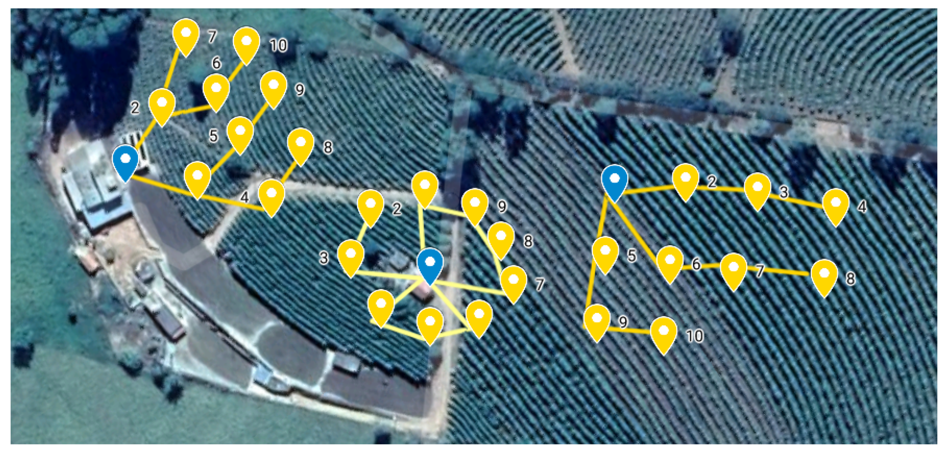
1. Introduction
2. Background
2.1. Wireless Sensor Networks
2.2. RPL
2.2.1. ETX Metric
- point-to-point communication:
- where the error probability () is:
- and the bidirectional communication is:
2.2.2. HOP Metric
3. Related Work
4. Evaluation Proposal and Analysis
4.1. Energy Consumption Evaluation
4.2. Simulation Parameters
4.3. Results and Analysis
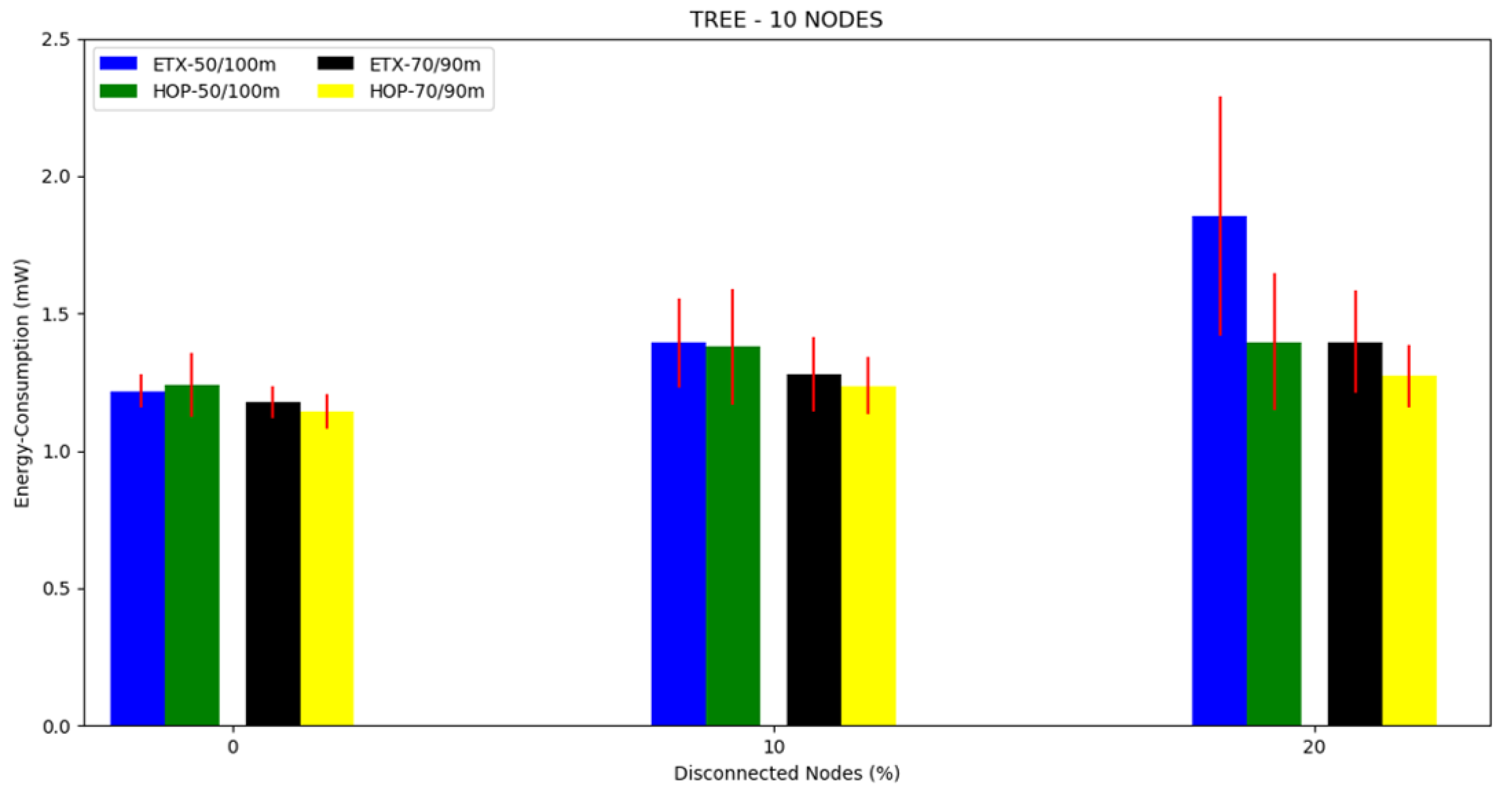
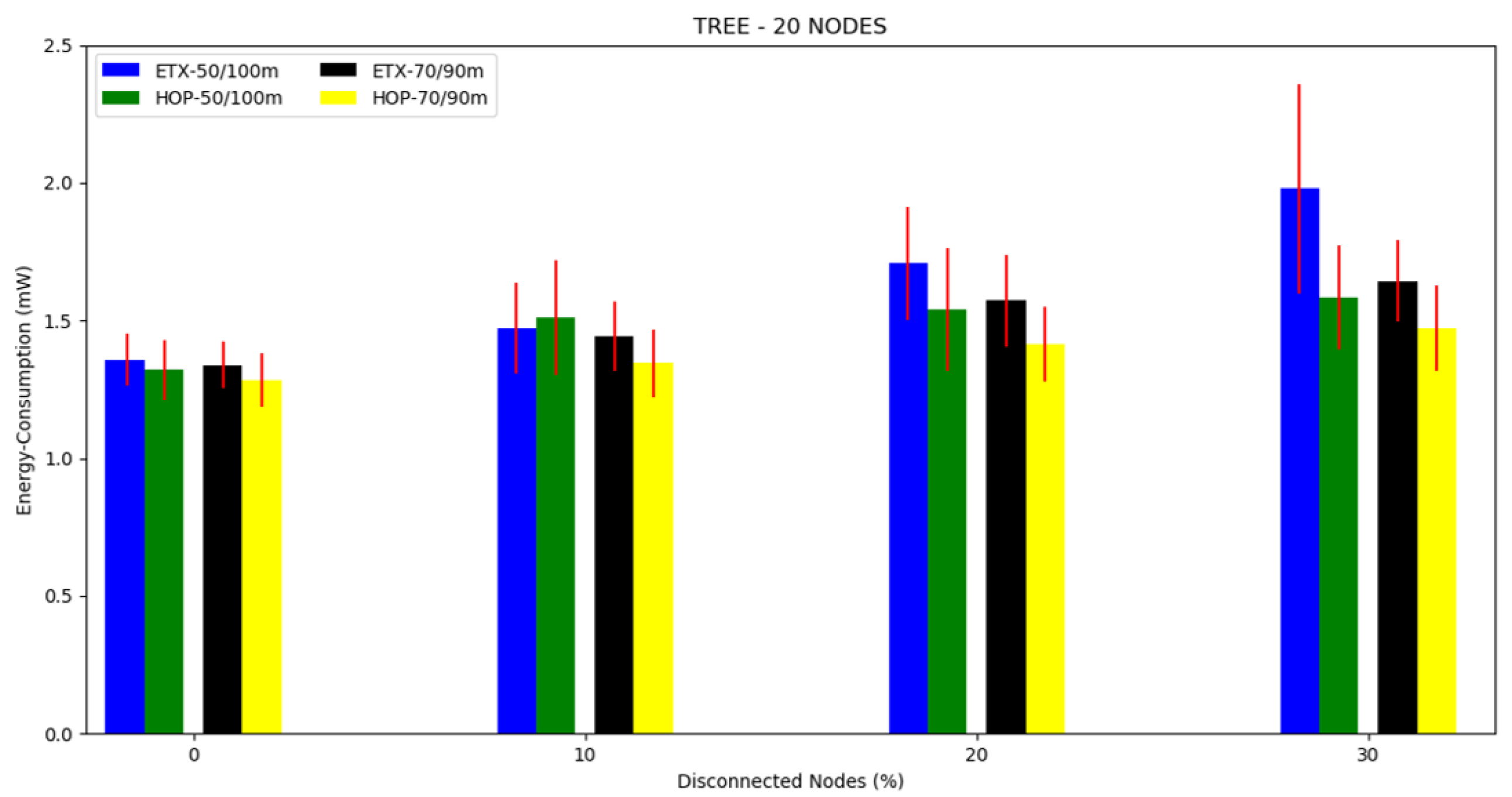
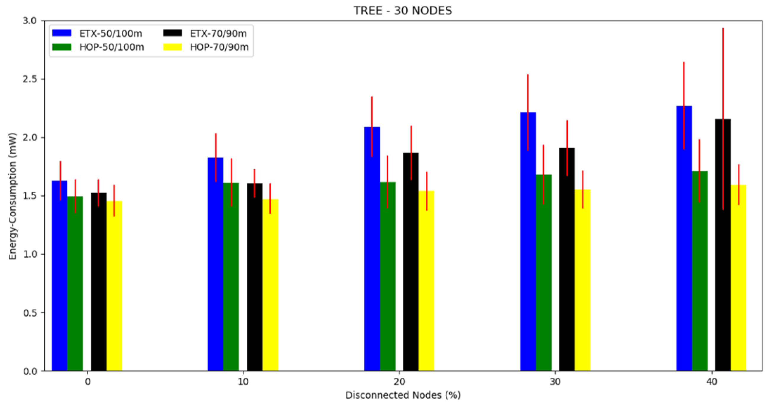
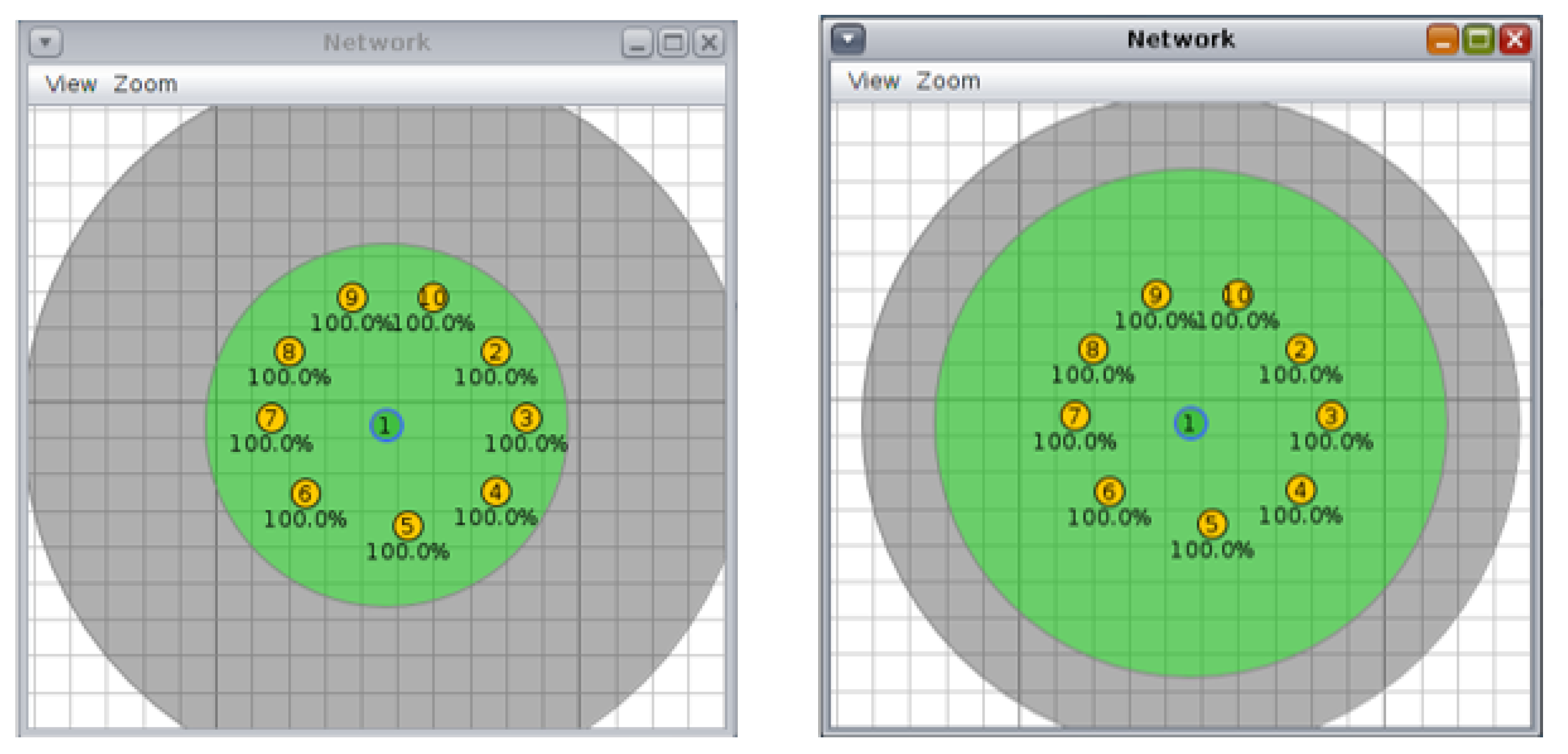
4.3.1. Tree Topology
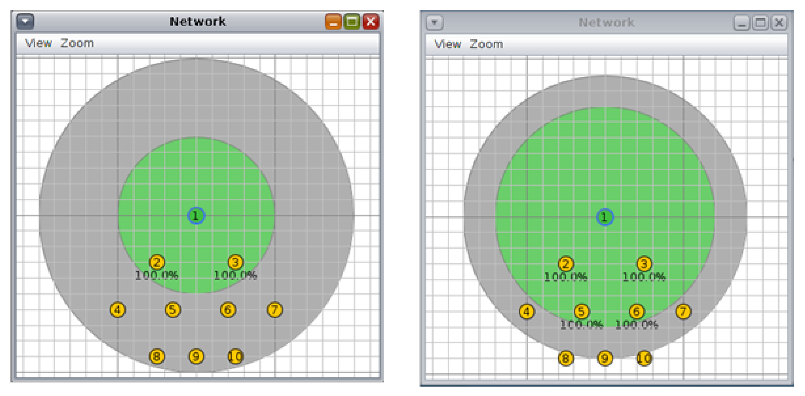
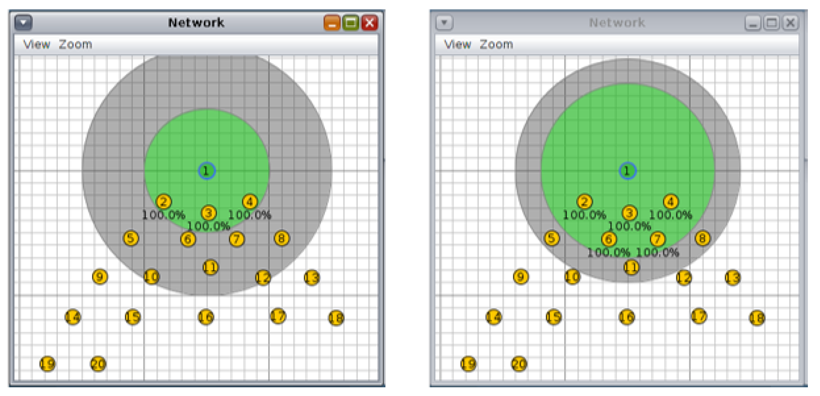
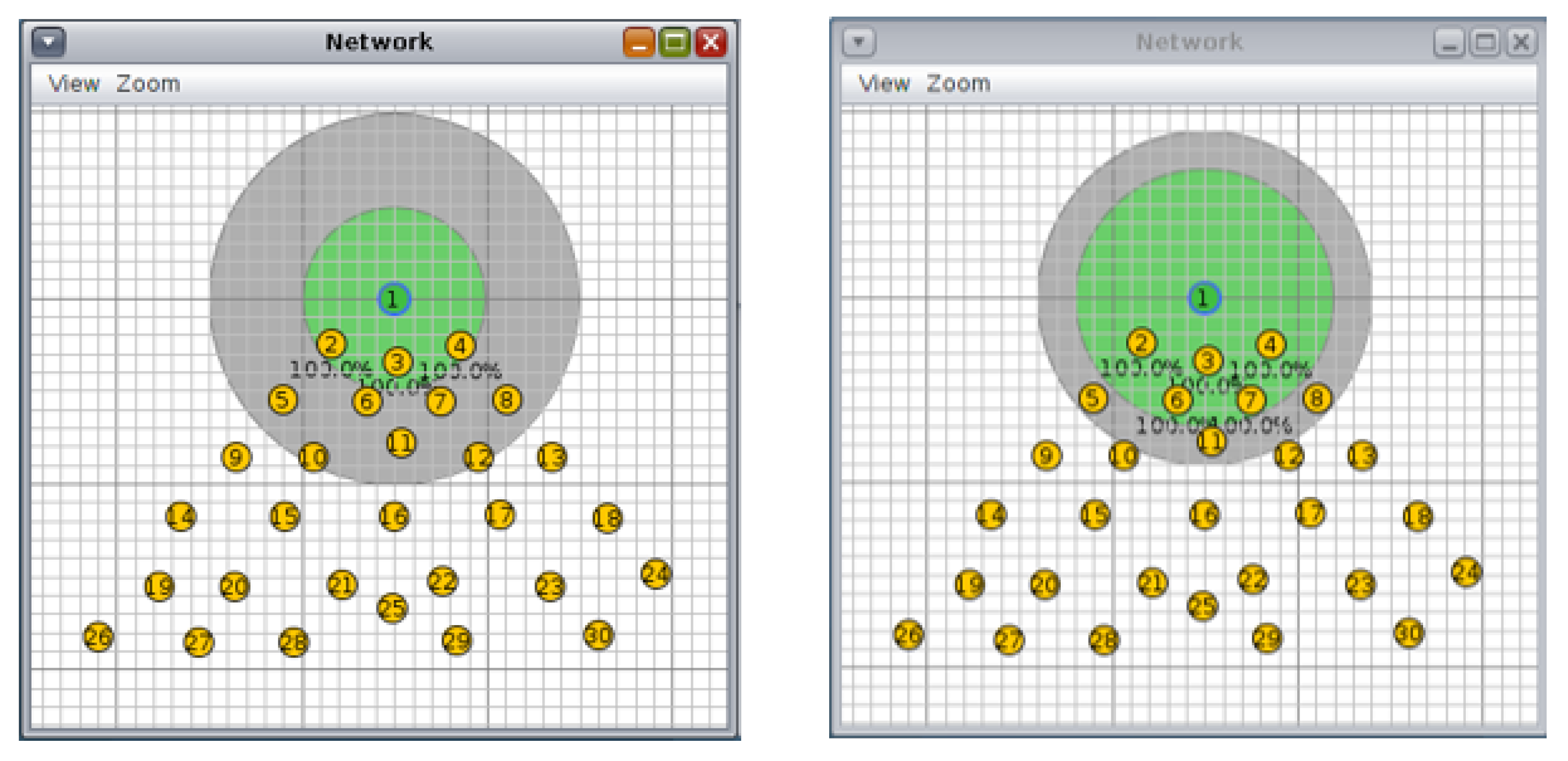
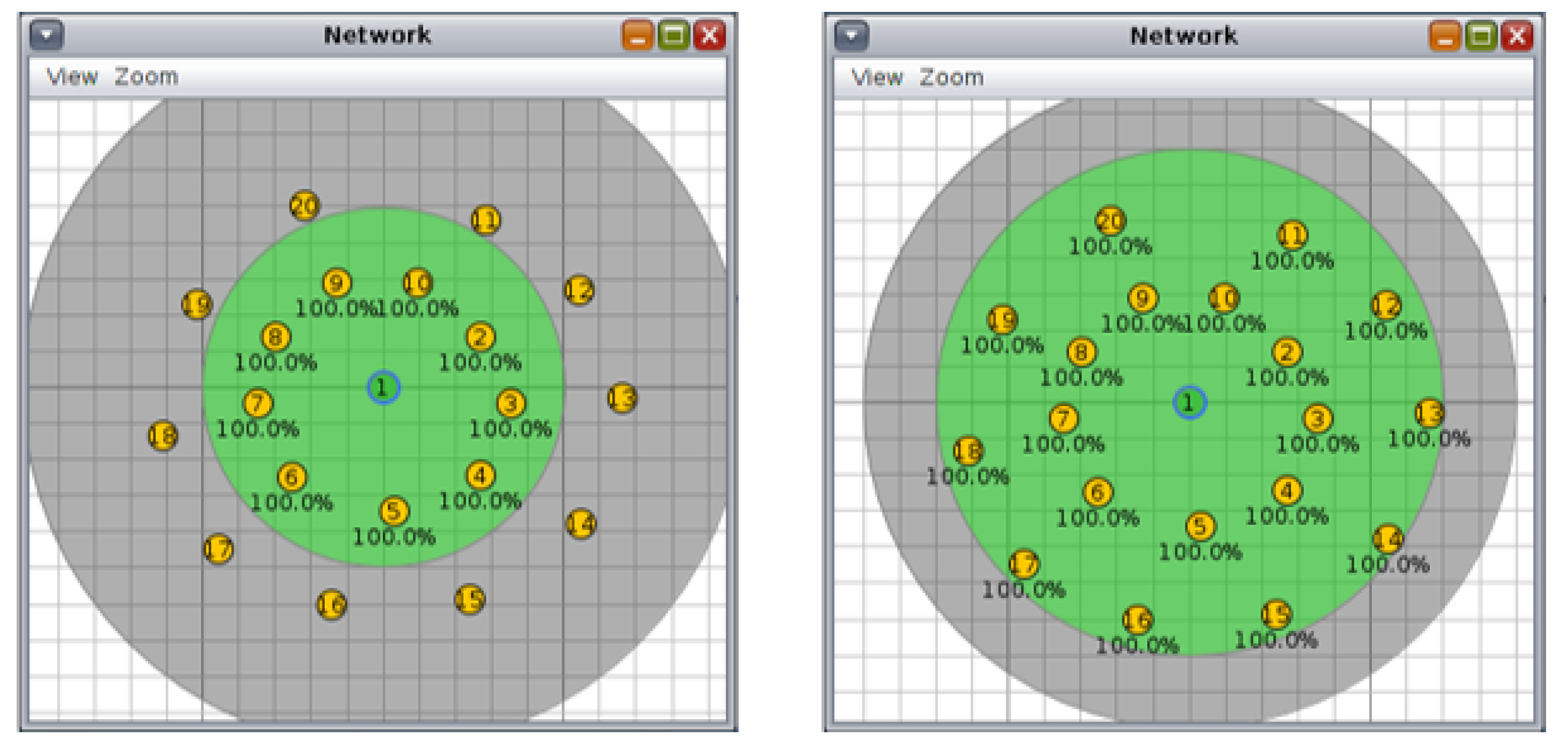
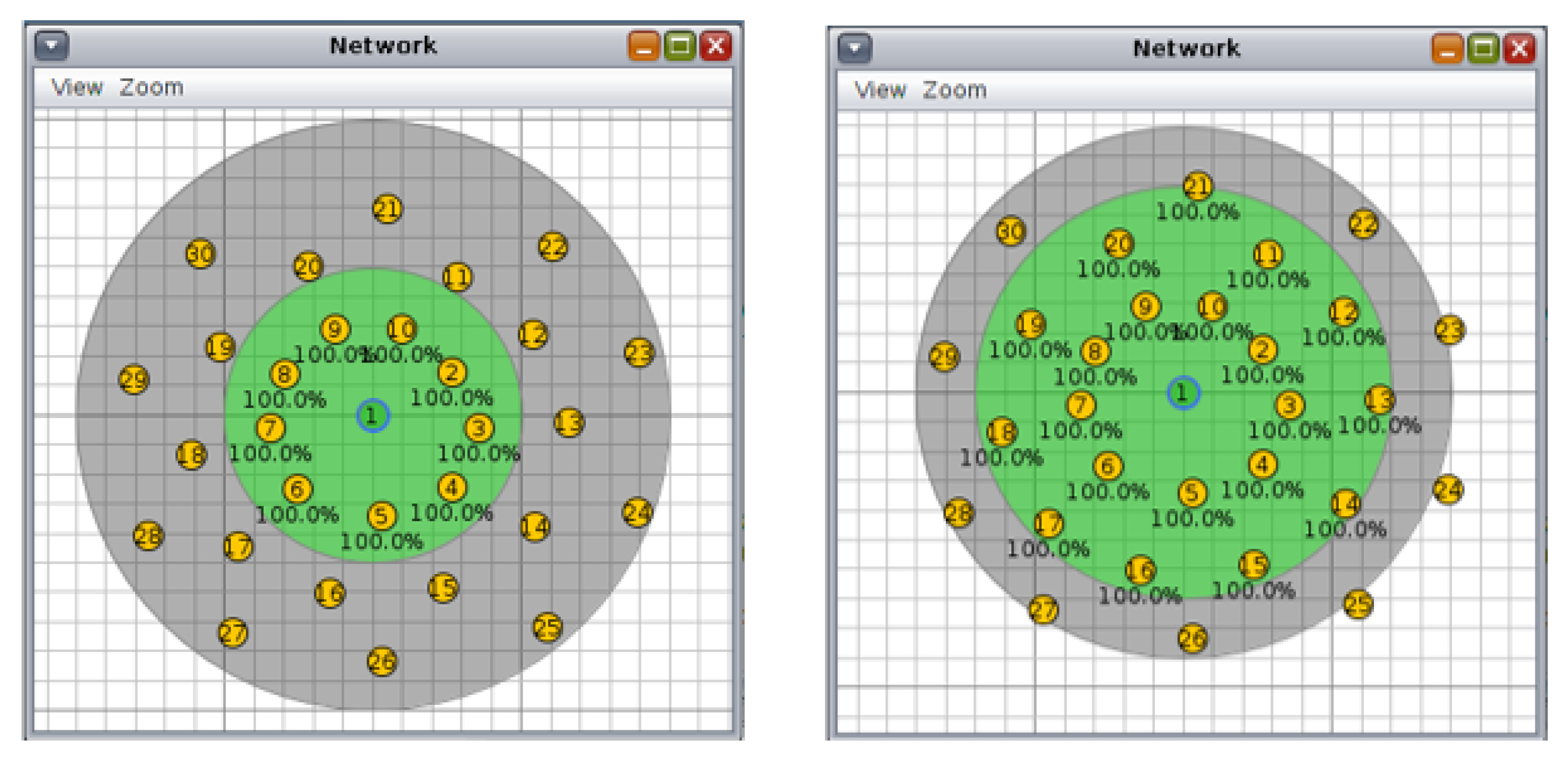
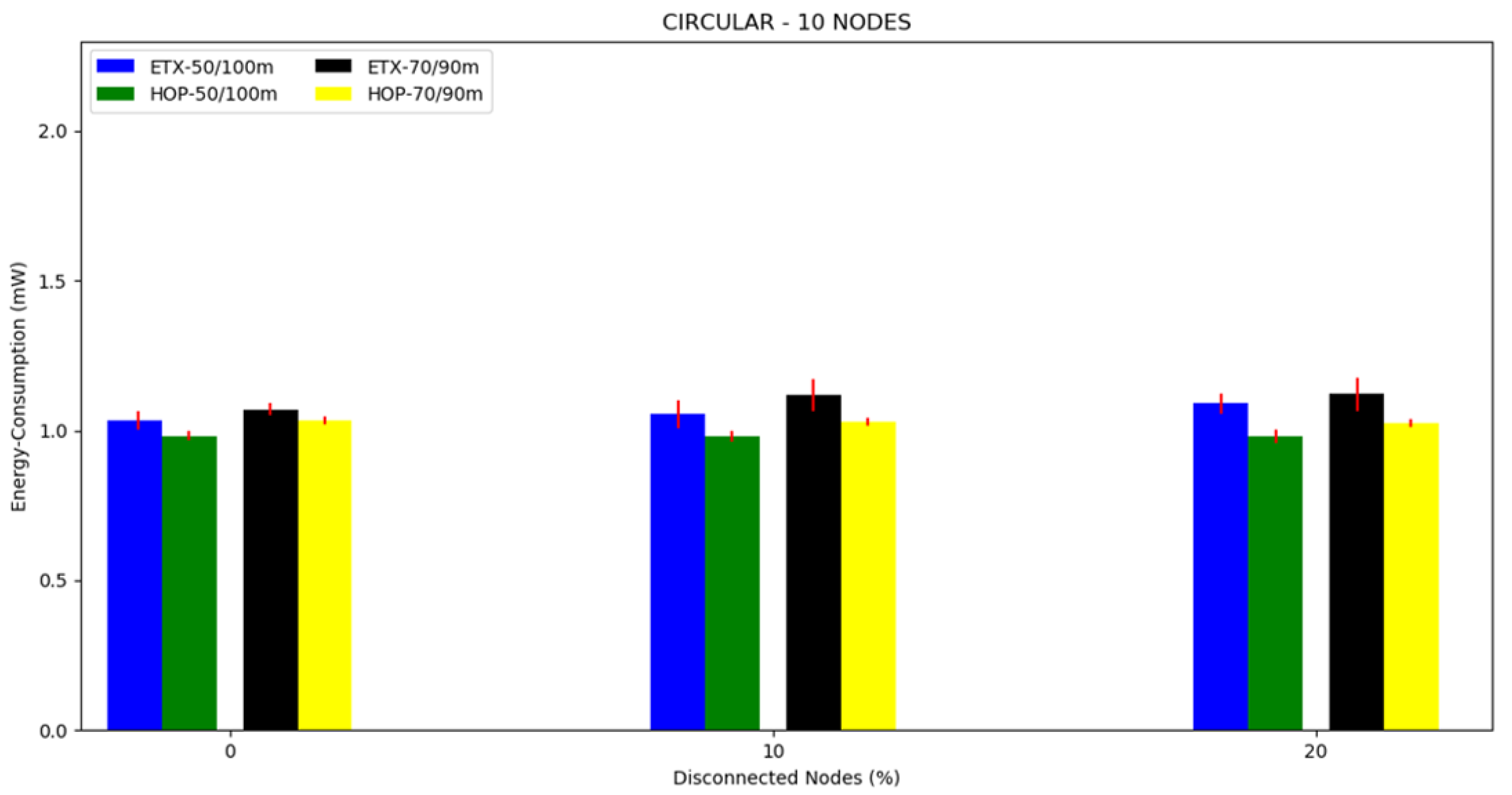
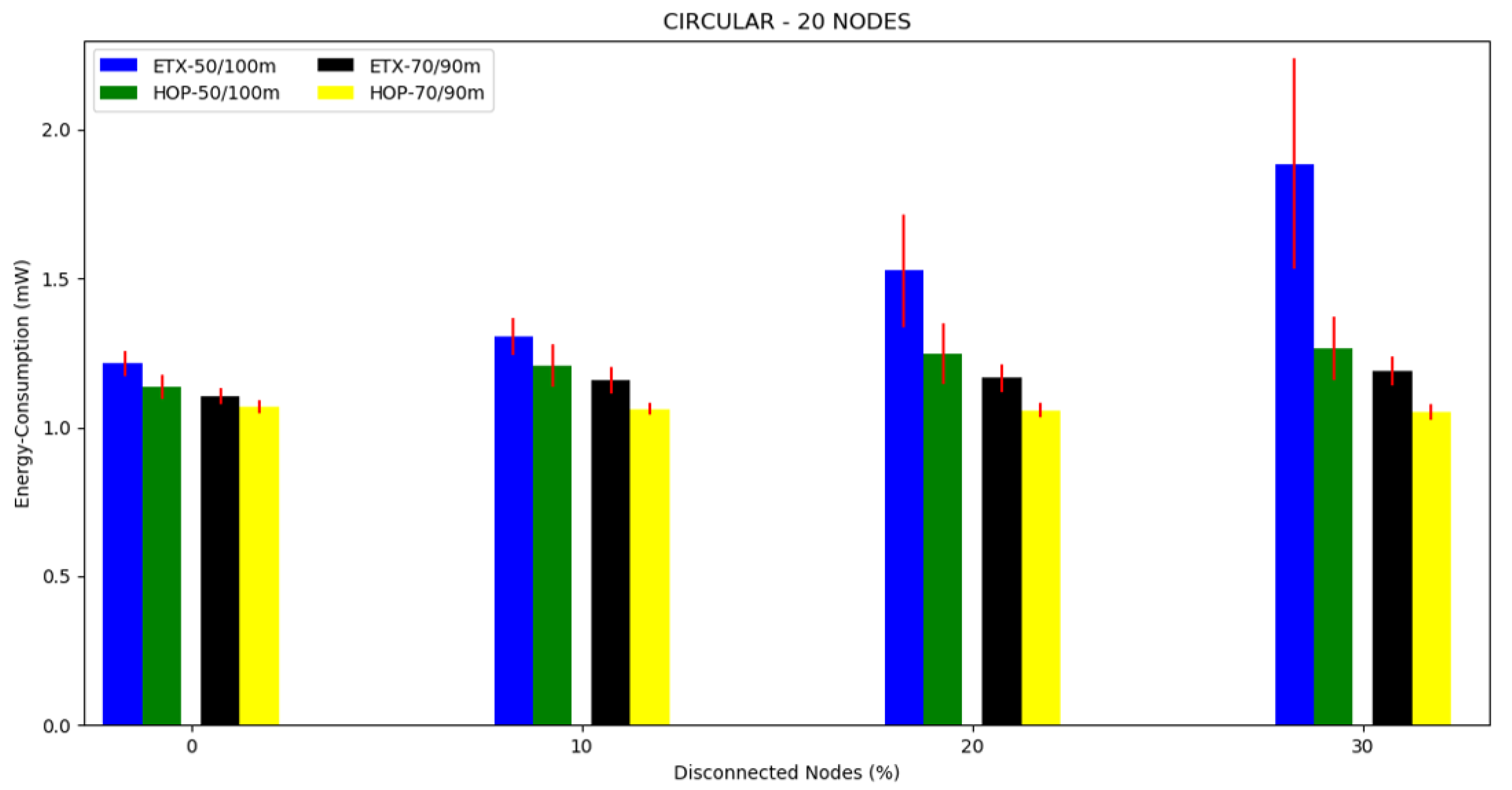
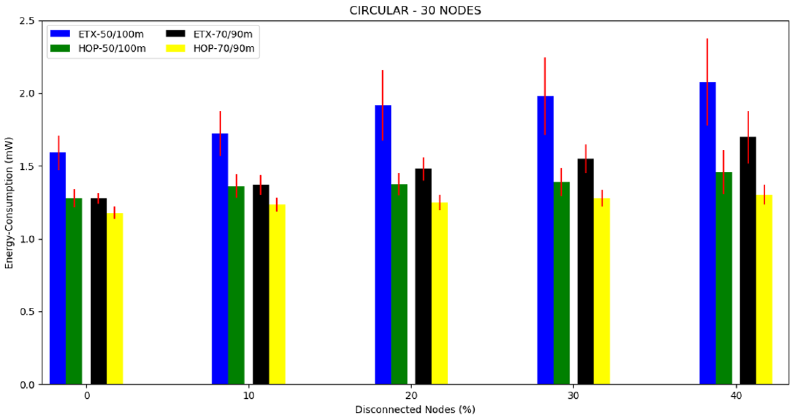
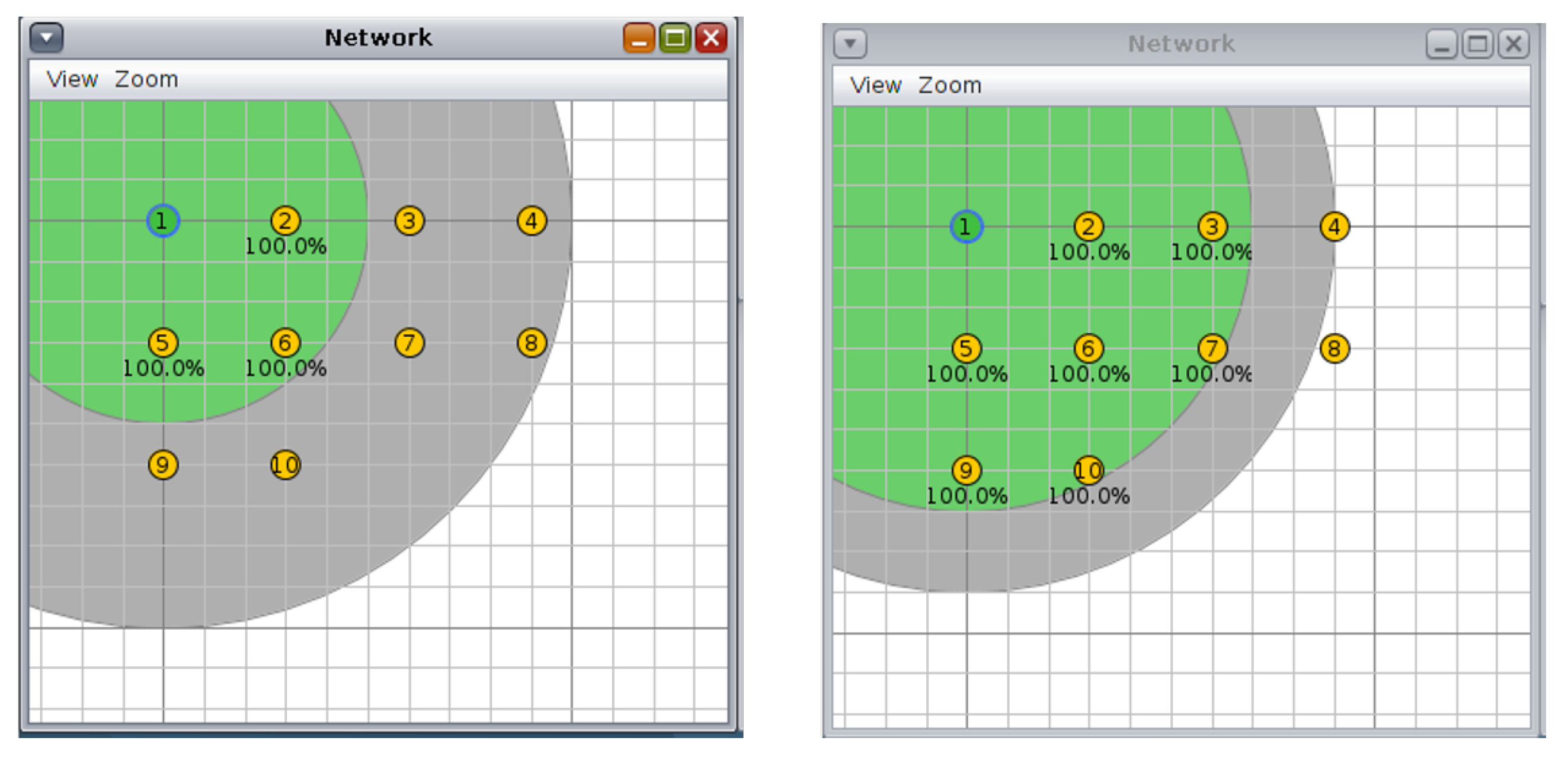
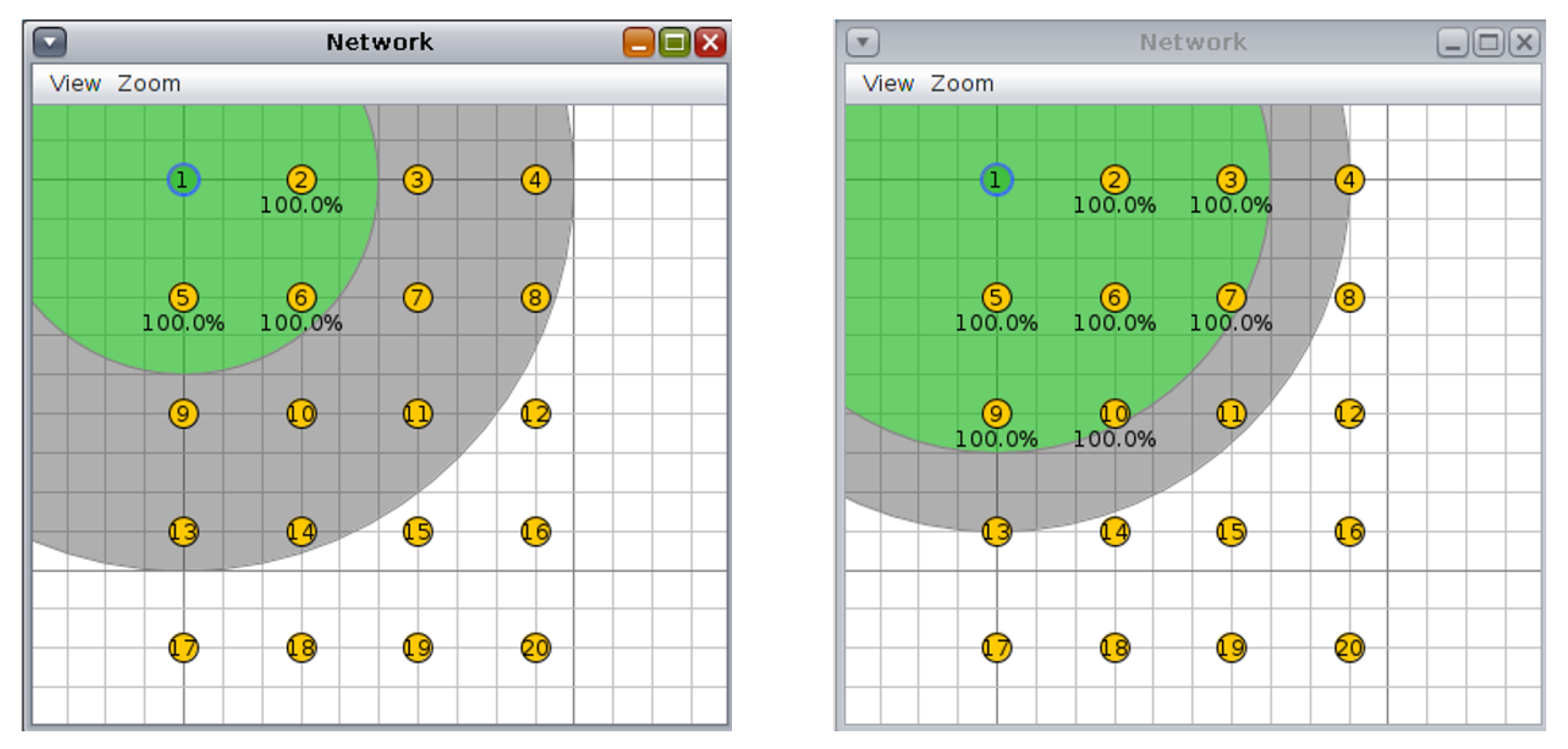
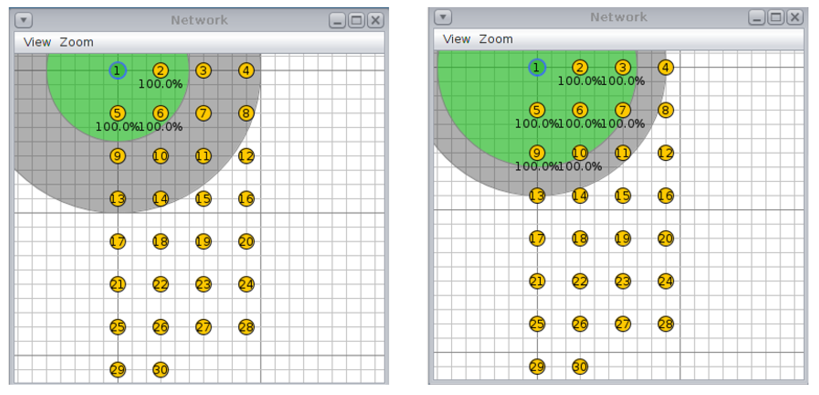
4.3.2. Circular Topology
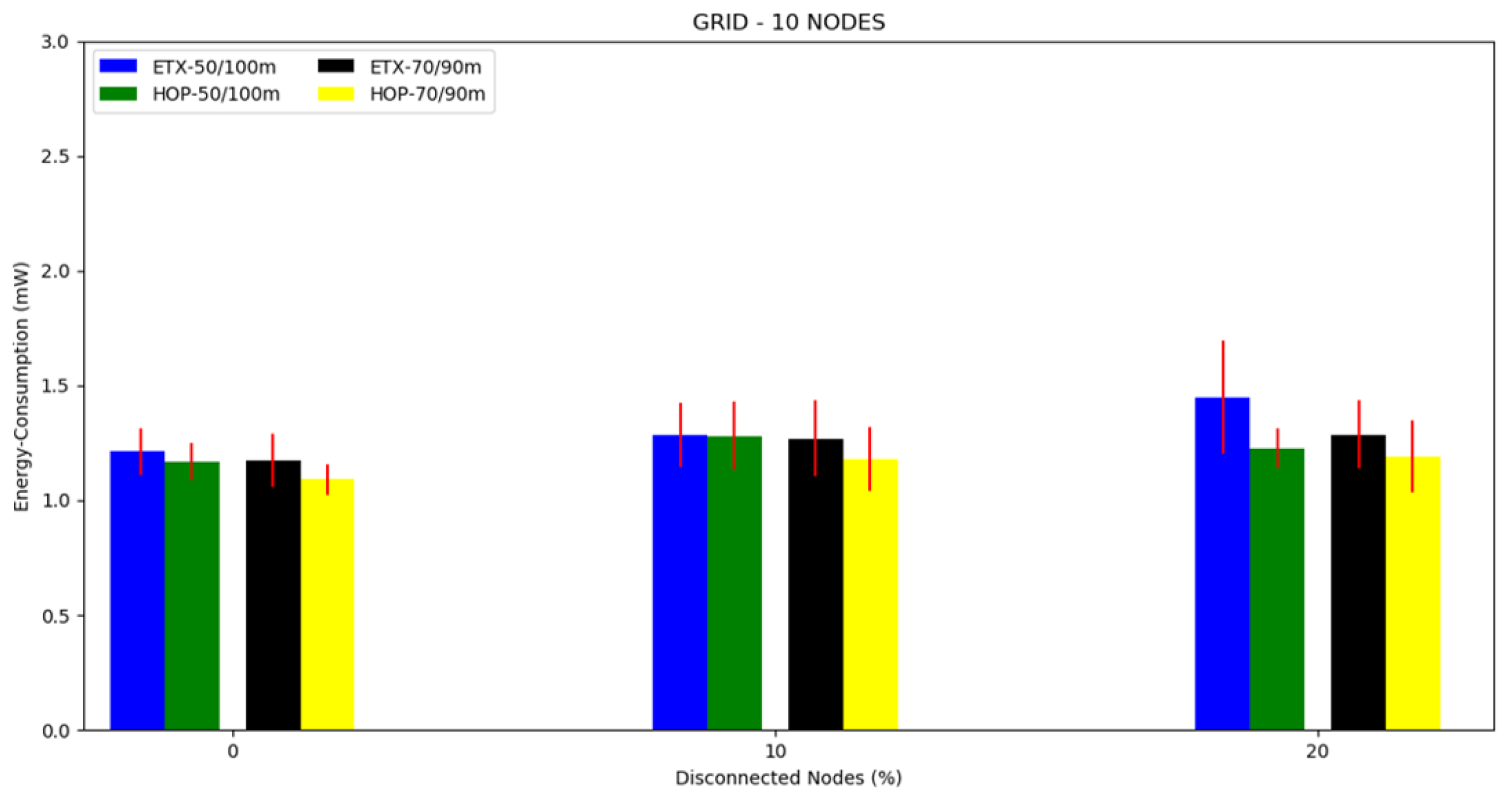
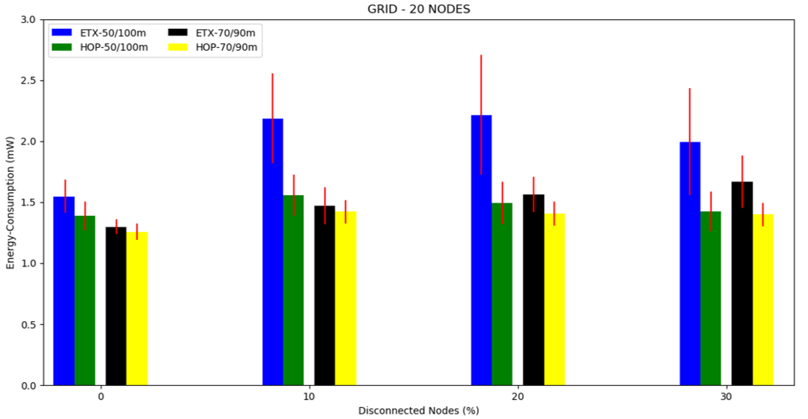
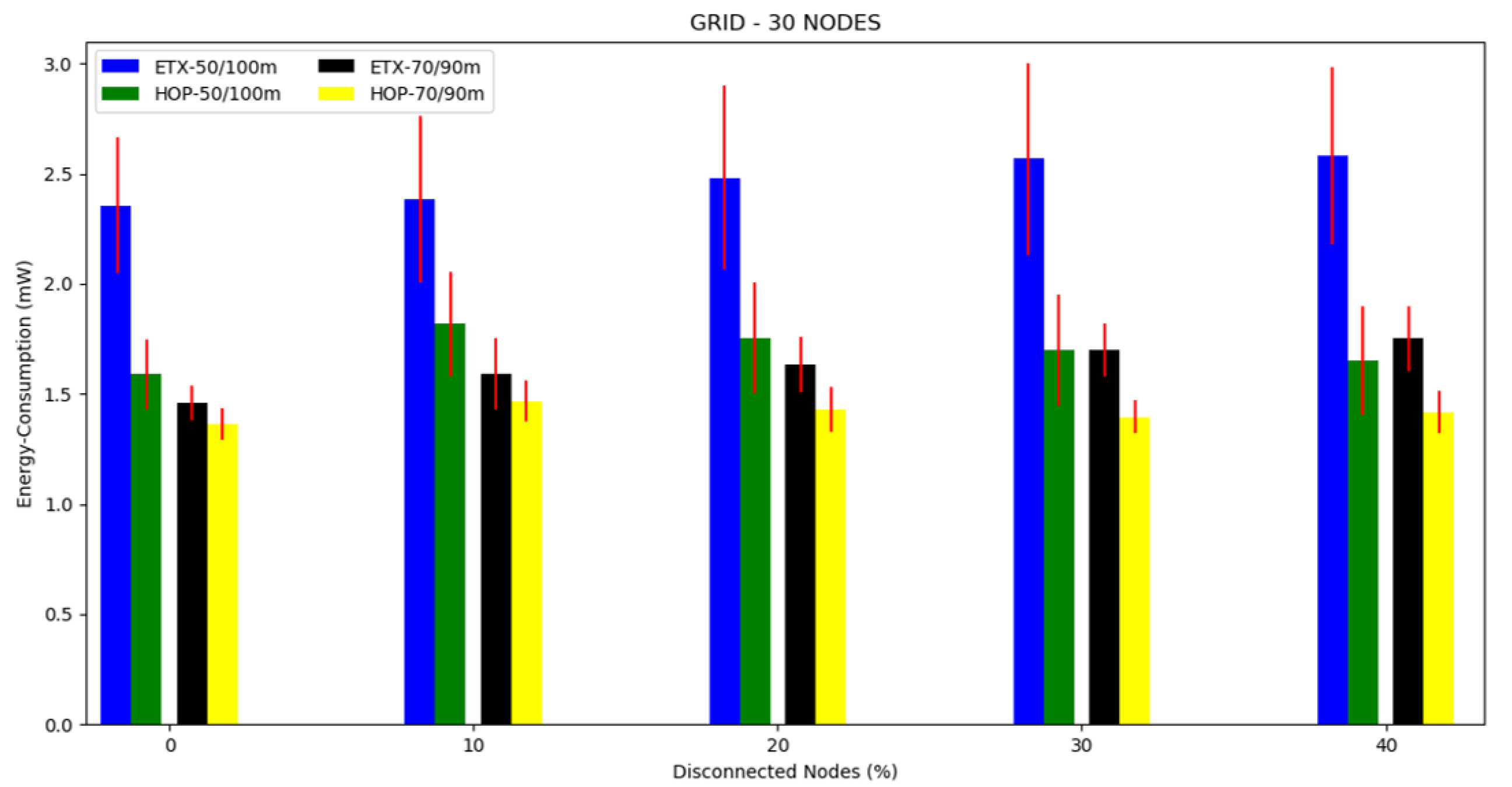
4.3.3. Grid Topology
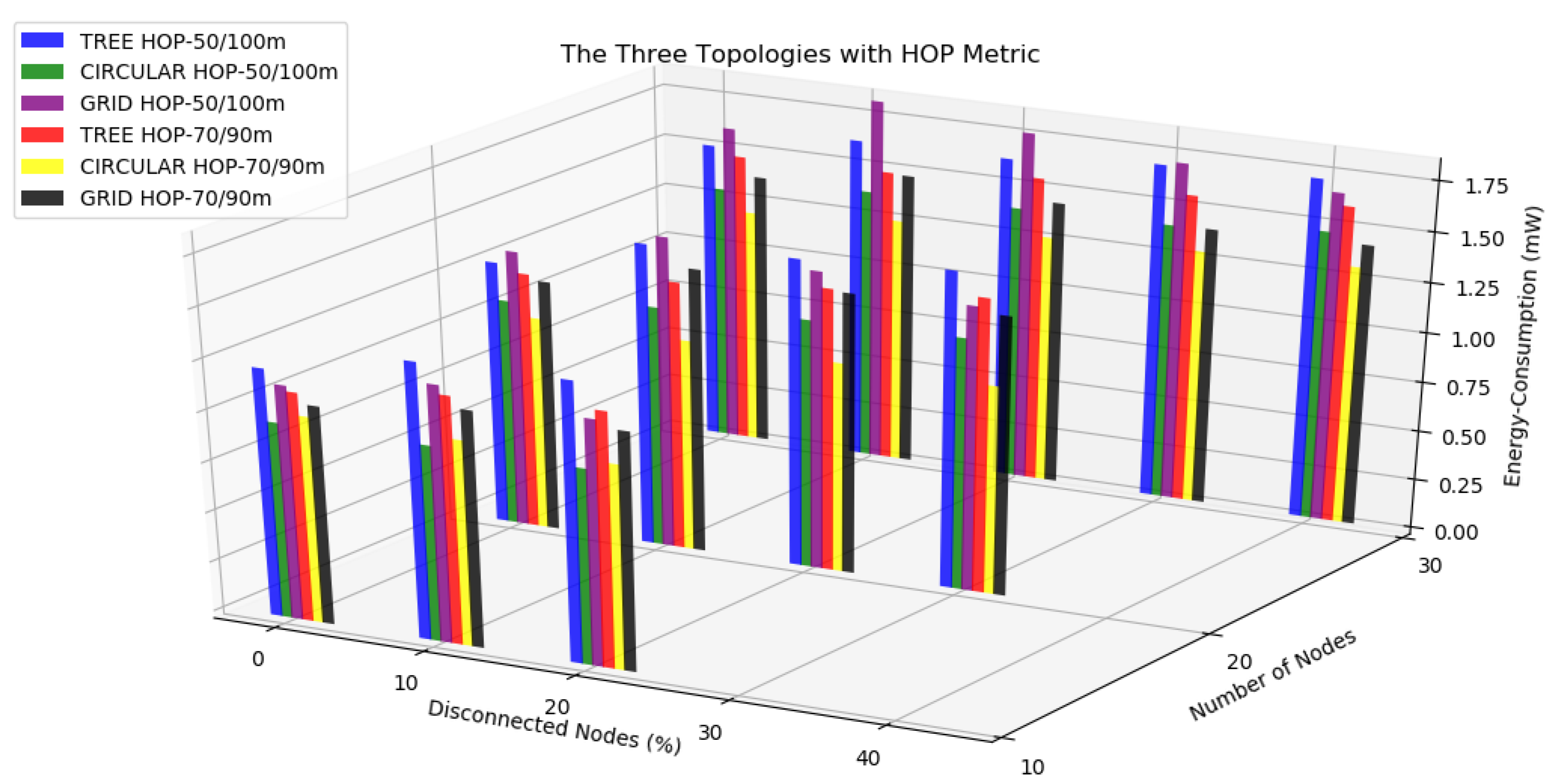
4.4. Discussion
5. Conclusions and Future Work
Author Contributions
Funding
Acknowledgments
Conflicts of Interest
References
- Yick, J.; Mukherjee, B.; Ghosal, D. Wireless sensor network survey. Comput. Networks 2008, 52, 2292–2330. [Google Scholar] [CrossRef]
- Dohler, M.; Barthel, D.; Maraninchi, F.; Mounier, L.; Aubert, S.; Dugas, C.; Buhrig, A.; Paugnat, F.; Renaudin, M.; Duda, A.; et al. The ARESA project: Facilitating research, development and commercialization of WSNs. In Proceedings of the 2007 4th Annual IEEE Communications Society Conference on Sensor, San Diego, CA, USA, 18–21 June 2007; pp. 590–599. [Google Scholar]
- Silva, E.F.; Dembogurski, B.J.; Vieira, A.B.; Ferreira, F.H.C. IEEE P21451-1-7: Providing more efficient network services over MQTT-SN. In Proceedings of the IEEE Sensors Applications Symposium, Sophia Antipolis, France, 11–13 March 2019; pp. 1–5. [Google Scholar]
- Bachir, A.; Dohler, M.; Watteyne, T.; Leung, K.K. MAC essentials for wireless sensor networks. IEEE Commun. Surv. Tutorials 2010, 12, 222–248. [Google Scholar] [CrossRef]
- Lampin, Q.; Barthel, D.; Valois, F. Efficient route redundancy in dag-based wireless sensor networks. In Proceedings of the Wireless Communications and Networking Conference (WCNC), Sydney, Australia, 18–21 April 2010; pp. 1–6. [Google Scholar]
- Watteyne, T.; Molinaro, A.; Richichi, M.G.; Dohler, M. From manet to ietf roll standardization: A paradigm shift in wsn routing protocols. IEEE Comm. Surv. Tutor. 2011, 13, 688–707. [Google Scholar] [CrossRef]
- Winter, T.; Thubert, P.; Brandt, A.; Hui, J.; Kelsey, R.; Levis, P.; Pister, K.; Struik, R.; Vasseur, J.P.; Alexander, R. RPL: IPv6 routing protocol for low-power and lossy networks. RFC 2012, 6550, 1–157. [Google Scholar]
- Alvi, S.A.; Ul Hassan, F.; Mian, A.N. On the energy efficiency and stability of RPL routing protocol. In Proceedings of the 2017 13th International Wireless Communications and Mobile Computing Conference (IWCMC), Valencia, Spain, 26–30 June 2017; pp. 927–1932. [Google Scholar]
- Javaid, N.; Javaid, A.; Khan, I.A.; Djouani, K. Performance study of ETX based wireless routing metrics. In Proceedings of the 2009 2nd International Conference on Computer, Control and Communication, Karachi, Pakistan, 17–18 February 2009. [Google Scholar]
- Nikodem, M.; Bawiec, M. Experimental Evaluation of Advertisement-Based Bluetooth Low Energy Communication. Sensors 2020, 20, 107. [Google Scholar] [CrossRef] [PubMed]
- Darroudi, S.M.; Gomez, C. Bluetooth low energy mesh networks: A survey. Sensors 2017, 17, 1467. [Google Scholar] [CrossRef] [PubMed]
- Basu, S.S.; Haxhibeqiri, J.; Baert, M.; Moons, B.; Karaagac, A.; Crombez, P.; Camerlynck, P.; Hoebeke, J. An End-To-End LwM2M-Based Communication Architecture for Multimodal NB-IoT/BLE Devices. Sensors 2020, 20, 2239. [Google Scholar] [CrossRef] [PubMed]
- Miguel, M.L.; Jamhour, E.; Pellenz, M.E.; Penna, M.C. A power planning algorithm based on rpl for ami wireless sensor networks. Sensors 2017, 17, 679. [Google Scholar] [CrossRef] [PubMed]
- Accettura, N.; Grieco, L.A.; Boggia, G.; Camarda, P. Performance analysis of the RPL routing protocol. In Proceedings of the 2011 IEEE International Conference on Mechatronics, Istanbul, Turkey, 13–15 April 2011; pp. 767–772. [Google Scholar]
- Tripathi, J.; De Oliveira, J.; Vasseur, J. Applicability study of RPL with local repair in smart grid substation networks. In Proceedings of the IEEE International Conference on Smart Grid Communications, Gaithersburg, MD, USA, 4–6 October 2010; pp. 262–267. [Google Scholar]
- Sharkawy, B.; Khattab, A.; Elsayed, K.M. Fault-tolerant RPL through context awareness. In Proceedings of the 2014 IEEE World Forum on Internet of Things (WF-IoT), Seoul, Korea, 6–8 March 2014; pp. 437–441. [Google Scholar]
- Thomson, C.; Wadhaj, I.; Romdhani, I.; Al-Dubai, A. Performance evaluation of RPL metrics in environments with strained transmission ranges. In Proceedings of the 2016 IEEE/ACS 13th International Conference of Computer Systems and Applications (AICCSA), Agadir, Morocco, 29 November–2 December 2016; pp. 1–8. [Google Scholar]
- Qasem, M.; Altawssi, H.; Yassien, M.B.; Al-Dubai, A. Performance evaluation of RPL objective functions. In Proceedings of the 2015 IEEE International Conference on Computer and Information Technology; Ubiquitous Computing and Communications; Dependable, Autonomic and Secure Computing; Pervasive Intelligence and Computing, Liverpool, UK, 26–28 October 2015; pp. 1606–1613. [Google Scholar]
- Thubert, P. Objective function zero for the routing protocol for low-power and lossy networks (RPL). RFC 2012, 6553, 1–14. [Google Scholar]
- Gnawali, O.; Levis, P. The minimum rank with hysteresis objective function. RFC 2012, 6719, 1–13. [Google Scholar]
- Jain, R. The Art of Computer Systems Performance Analysis: Techniques for Experimental Design, Measurement, Simulation, and Modeling. SIGMETRICS Perform. Evaluation Rev.. 1991, Volume 19, pp. 5–11. Available online: https://www.cse.wustl.edu/~jain/books/perfbook.htm (accessed on 2 July 2020).
- Dunkels, A. Contiki: The Open Source Operating System for the Internet of Things. Available online: http://www.contiki-os.org/ (accessed on 29 April 2019).
- Yi, J.; De Verdiere, A.C.; Igarashi, Y.; Morii, Y. Lightweight On-demand Ad hoc Distance-vector Routing–Next Generation (LOADng): Protocol, extension, and applicability. Comput. Netw. 2017, 126, 125–140. [Google Scholar]
- Sobral, J.V.; Rodrigues, J.J.; Rabêlo, R.A.; Saleem, K.; Furtado, V. LOADng-IoT: An enhanced routing protocol for internet of things applications over low power networks. Sensors 2019, 19, 150. [Google Scholar] [CrossRef] [PubMed]
- Silva, E.F.; Muchaluat-Saade, D.C.; Fernandes, N.C. ACROSS: A generic framework for attribute-based access control with distributed policies for virtual organizations. Future Gener. Comput. Syst. 2018, 78, 1–17. [Google Scholar] [CrossRef]


| Parameters | Values | |
|---|---|---|
| Objective Functions | OF0 | MRHOF |
| Metrics | HOP | ETX |
| Transmission/interference ranges | 50/100 m, 70/90 m | |
| Topologies | Tree, circular, grid | |
| Simulation duration | 10 min | |
| Number of nodes | 10, 20, and 30 | |
| Type of nodes | Sky Mote | |
| Wireless channel model | UDGM | |
| Energy Consumption (mW) | Energy Consumption (mW) | ||||||
|---|---|---|---|---|---|---|---|
| Number of Nodes | Disconnected Nodes (%) | Transmission/ Interference | ETX | HOP | Transmission/ Interference | ETX | HOP |
| 10 | 0 | 50/100 m | 1.2173 | 1.2386 | 70/90 m | 1.1774 | 1.1434 |
| 10 | 1.3928 | 1.3777 | 1.2768 | 1.2367 | |||
| 20 | 1.8560 | 1.3957 | 1.3965 | 1.2715 | |||
| 20 | 0 | 50/100 m | 1.3576 | 1.3200 | 70/90 m | 1.3386 | 1.2832 |
| 10 | 1.4709 | 1.5115 | 1.4430 | 1.3438 | |||
| 20 | 1.7069 | 1.5385 | 1.5716 | 1.4149 | |||
| 30 | 1.9783 | 1.5827 | 1.6428 | 1.4723 | |||
| 30 | 0 | 50/100 m | 1.6277 | 1.4936 | 70/90 m | 1.5241 | 1.4550 |
| 10 | 1.8235 | 1.6107 | 1.6044 | 1.4718 | |||
| 20 | 2.0865 | 1.6153 | 1.8650 | 1.5381 | |||
| 40 | 2.2123 | 1.6809 | 1.9048 | 1.5501 | |||
| 50 | 2.2674 | 1.7096 | 2.1557 | 1.5930 | |||
| Energy Consumption (mW) | Energy Consumption (mW) | ||||||
|---|---|---|---|---|---|---|---|
| Number of Nodes | Disconnected Nodes (%) | Transmission/ Interference | ETX | HOP | Transmission/ Interference | ETX | HOP |
| 10 | 0 | 50/100 m | 1.0352 | 0.9807 | 70/90 m | 1.0714 | 1.0322 |
| 10 | 1.0542 | 0.9790 | 1.1173 | 1.0286 | |||
| 20 | 1.0895 | 0.9792 | 1.1222 | 1.0230 | |||
| 20 | 0 | 50/100 m | 1.2143 | 1.1361 | 70/90 m | 1.1039 | 1.0688 |
| 10 | 1.3056 | 1.2062 | 1.1576 | 1.0615 | |||
| 20 | 1.5256 | 1.2476 | 1.1650 | 1.0568 | |||
| 30 | 1.8854 | 1.2637 | 1.1884 | 1.0500 | |||
| 30 | 0 | 50/100 m | 1.5911 | 1.2786 | 70/90 m | 1.2773 | 1.1778 |
| 10 | 1.7239 | 1.3621 | 1.3690 | 1.2342 | |||
| 20 | 1.9176 | 1.3756 | 1.4777 | 1.2500 | |||
| 40 | 1.9779 | 1.3902 | 1.5488 | 1.2792 | |||
| 50 | 2.0759 | 1.4568 | 1.6978 | 1.3020 | |||
| Energy Consumption (mW) | Energy Consumption (mW) | ||||||
|---|---|---|---|---|---|---|---|
| Number of Nodes | Disconnected Nodes (%) | Transmission/ Interference | ETX | HOP | Transmission/ Interference | ETX | HOP |
| 10 | 0 | 50/100 m | 1.2124 | 1.1705 | 70/90 m | 1.1744 | 1.0915 |
| 10 | 1.2842 | 1.2812 | 1.2697 | 1.1806 | |||
| 20 | 1.4484 | 1.2248 | 1.2868 | 1.1899 | |||
| 20 | 0 | 50/100 m | 1.5482 | 1.3864 | 70/90 m | 1.2977 | 1.2575 |
| 10 | 2.1861 | 1.5578 | 1.4724 | 1.4210 | |||
| 20 | 2.2158 | 1.4922 | 1.5615 | 1.4058 | |||
| 30 | 1.9948 | 1.4259 | 1.6700 | 1.3994 | |||
| 30 | 0 | 50/100 m | 2.3544 | 1.5900 | 70/90 m | 1.4585 | 1.3630 |
| 10 | 2.3837 | 1.8175 | 1.5898 | 1.4666 | |||
| 20 | 2.4808 | 1.7541 | 1.6330 | 1.4277 | |||
| 40 | 2.5662 | 1.7010 | 1.6993 | 1.3954 | |||
| 50 | 2.5825 | 1.6530 | 1.7517 | 1.4167 | |||
© 2020 by the authors. Licensee MDPI, Basel, Switzerland. This article is an open access article distributed under the terms and conditions of the Creative Commons Attribution (CC BY) license (http://creativecommons.org/licenses/by/4.0/).
Share and Cite
O. Sales, F.; Marante, Y.; Vieira, A.B.; Silva, E.F. Energy Consumption Evaluation of a Routing Protocol for Low-Power and Lossy Networks in Mesh Scenarios for Precision Agriculture. Sensors 2020, 20, 3814. https://doi.org/10.3390/s20143814
O. Sales F, Marante Y, Vieira AB, Silva EF. Energy Consumption Evaluation of a Routing Protocol for Low-Power and Lossy Networks in Mesh Scenarios for Precision Agriculture. Sensors. 2020; 20(14):3814. https://doi.org/10.3390/s20143814
Chicago/Turabian StyleO. Sales, Frederico, Yelco Marante, Alex B. Vieira, and Edelberto Franco Silva. 2020. "Energy Consumption Evaluation of a Routing Protocol for Low-Power and Lossy Networks in Mesh Scenarios for Precision Agriculture" Sensors 20, no. 14: 3814. https://doi.org/10.3390/s20143814
APA StyleO. Sales, F., Marante, Y., Vieira, A. B., & Silva, E. F. (2020). Energy Consumption Evaluation of a Routing Protocol for Low-Power and Lossy Networks in Mesh Scenarios for Precision Agriculture. Sensors, 20(14), 3814. https://doi.org/10.3390/s20143814