Estimating Blood Pressure from the Photoplethysmogram Signal and Demographic Features Using Machine Learning Techniques

 ,
,  ,
,  , and
, and
Abstract
1. Introduction
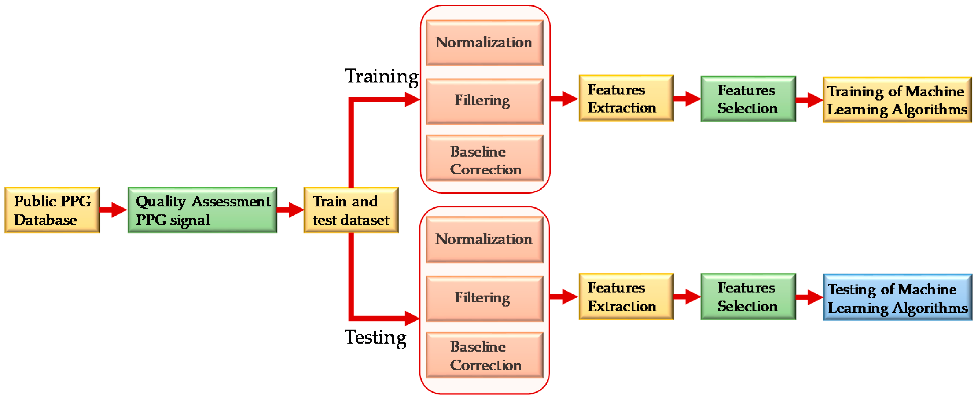
2. Materials and Methods
2.1. Dataset Description
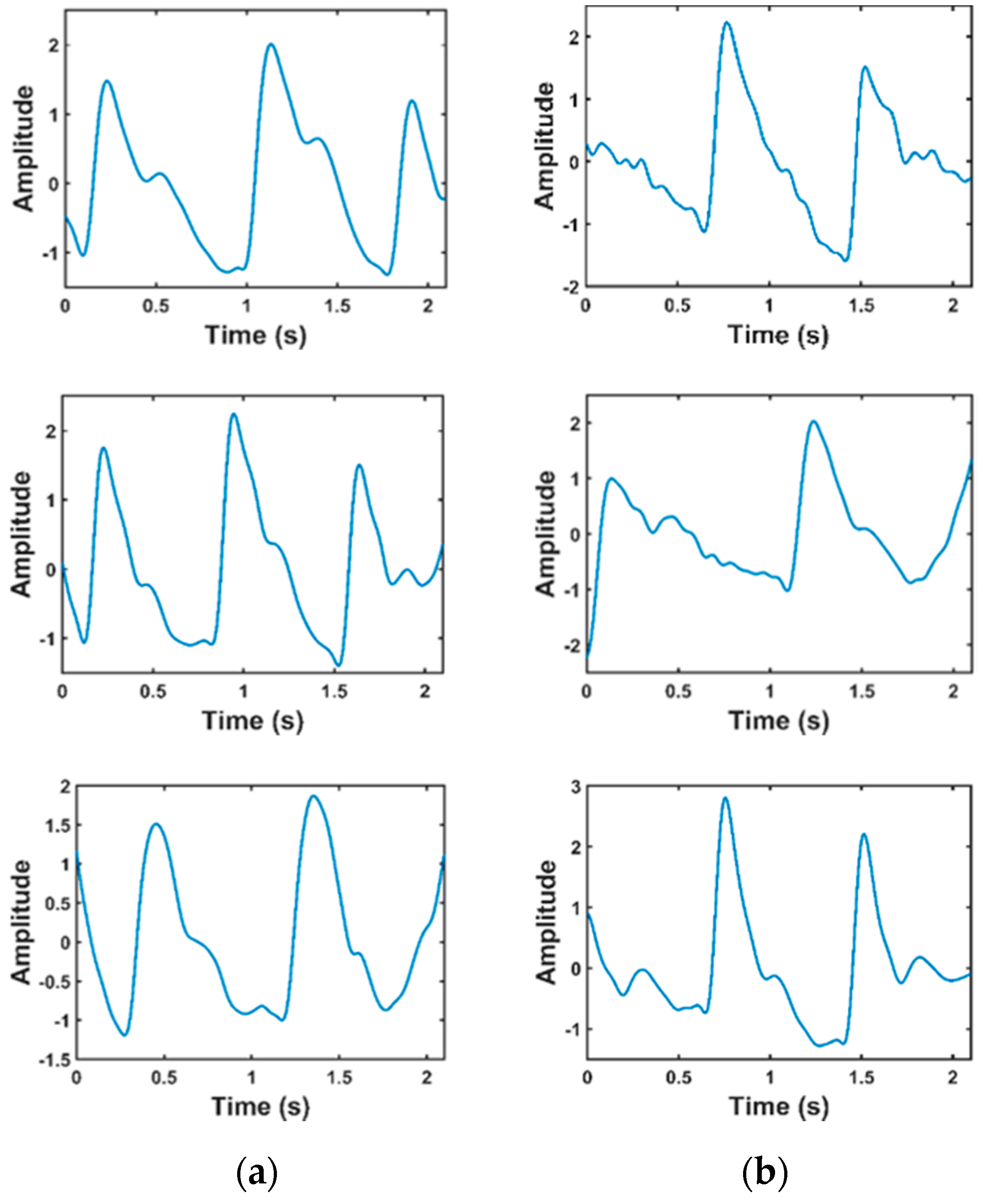
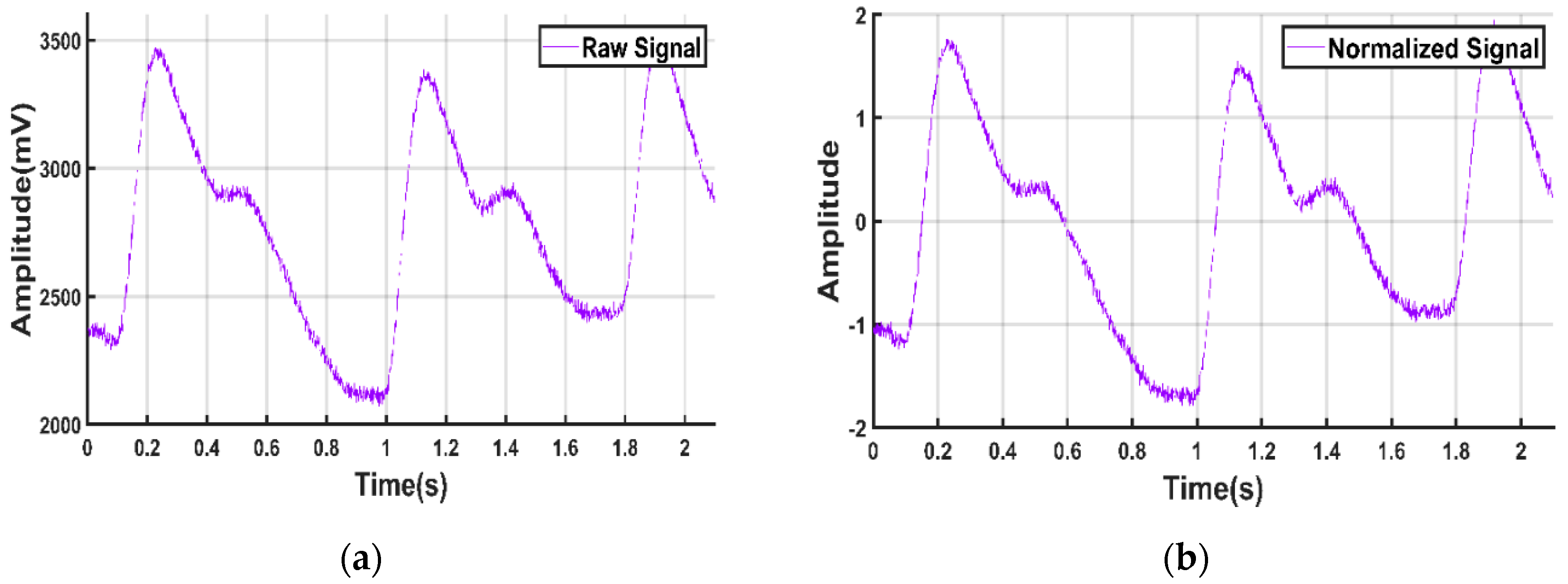
2.2. Preprocessing Signals
2.2.1. Normalization
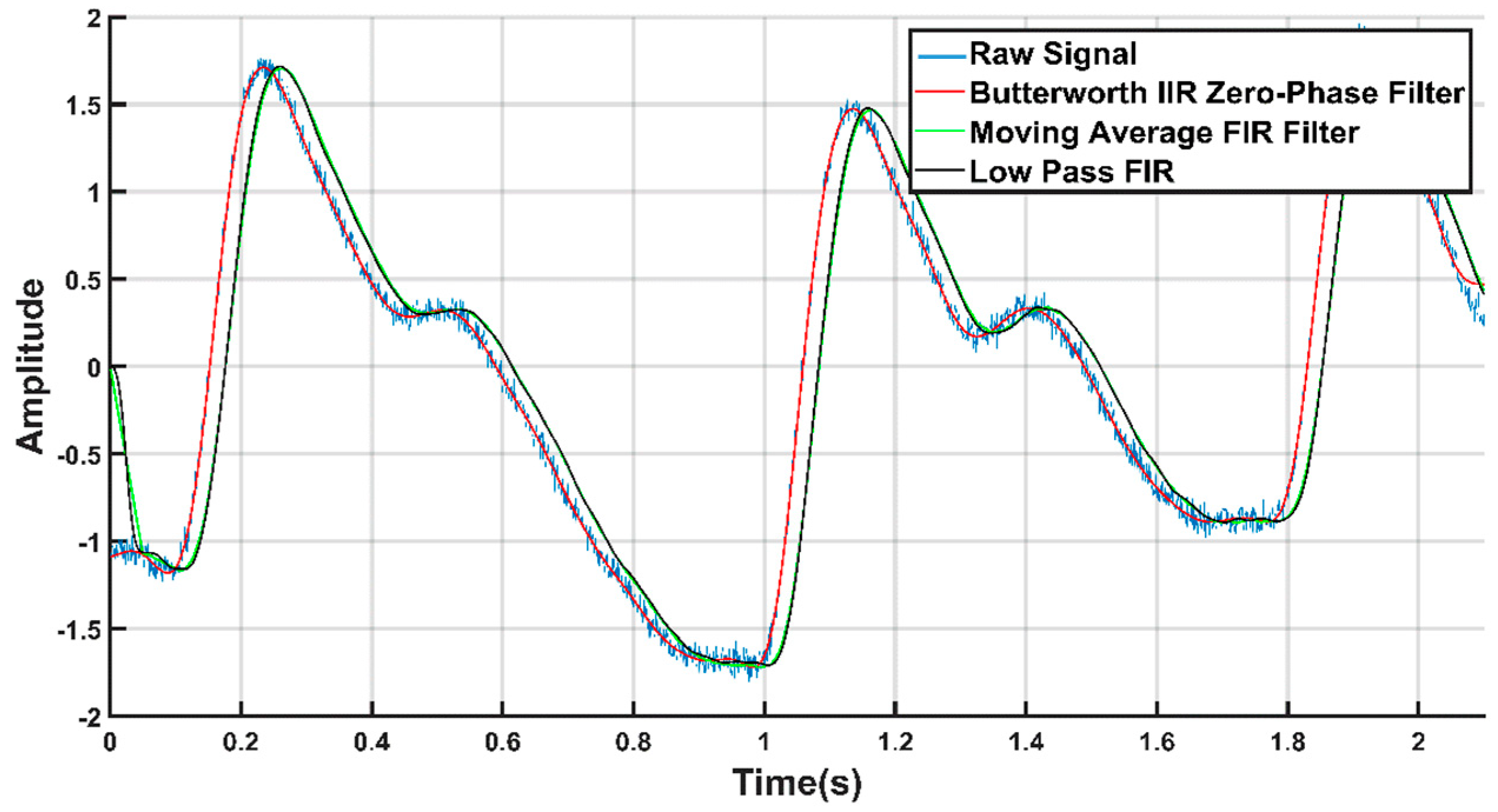
2.2.2. Signal Filtration
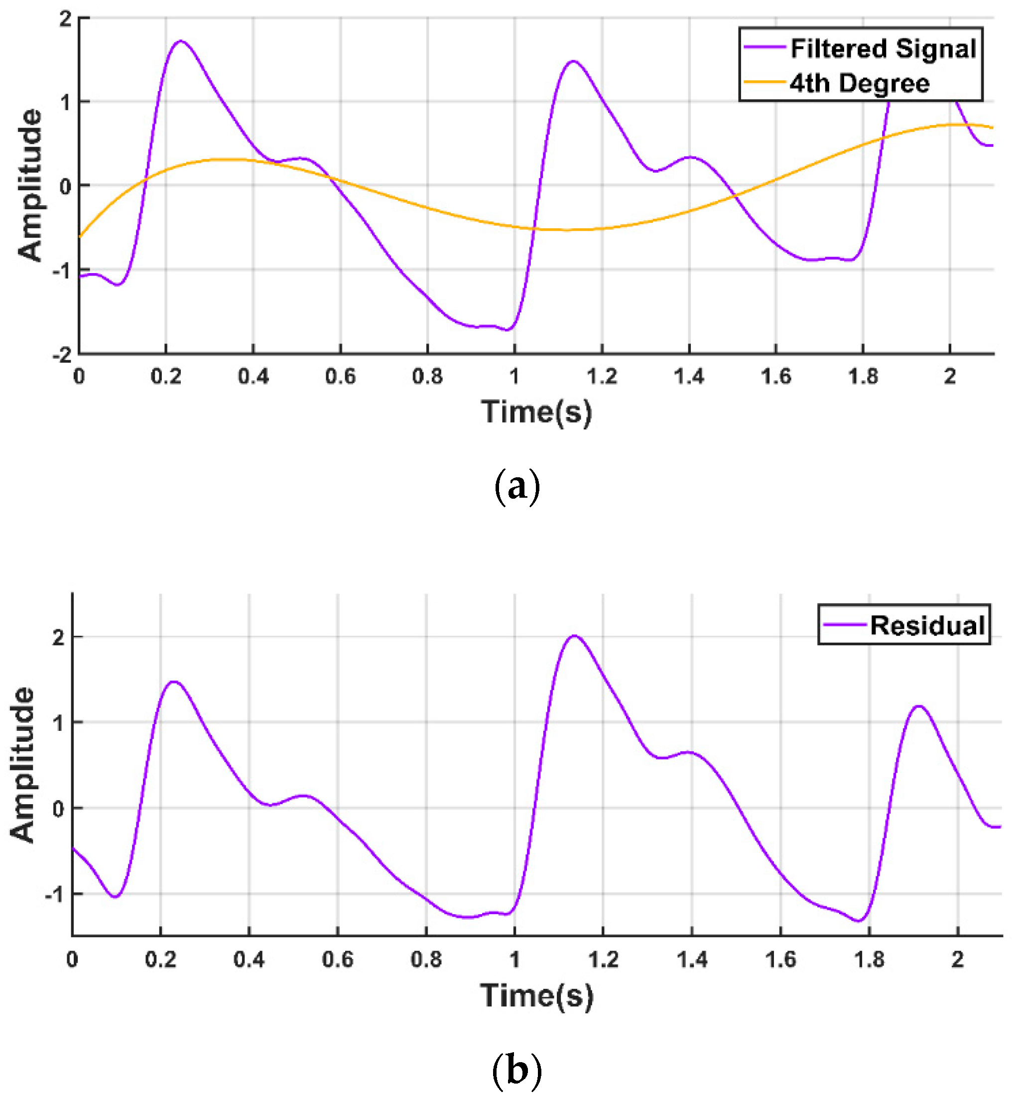
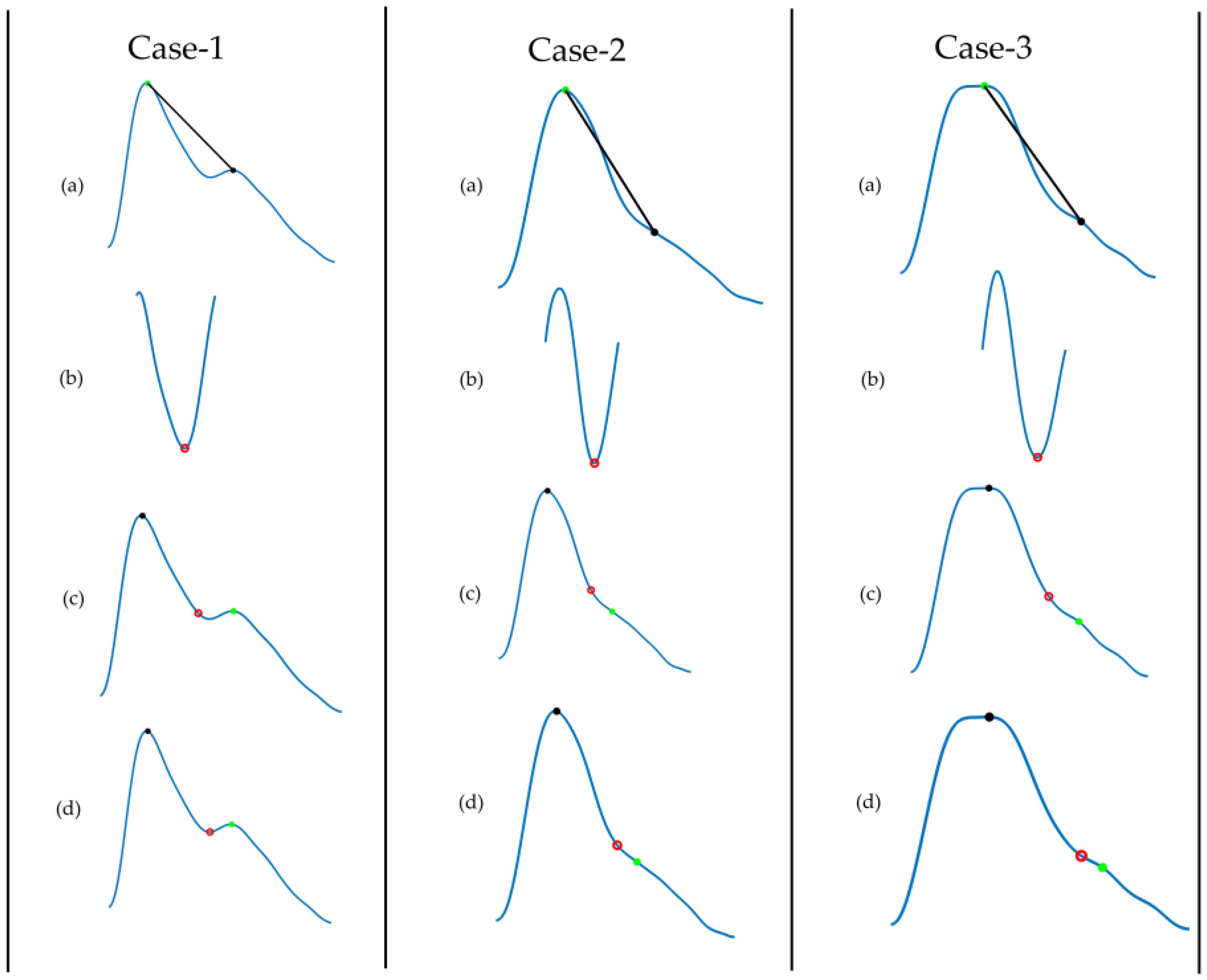
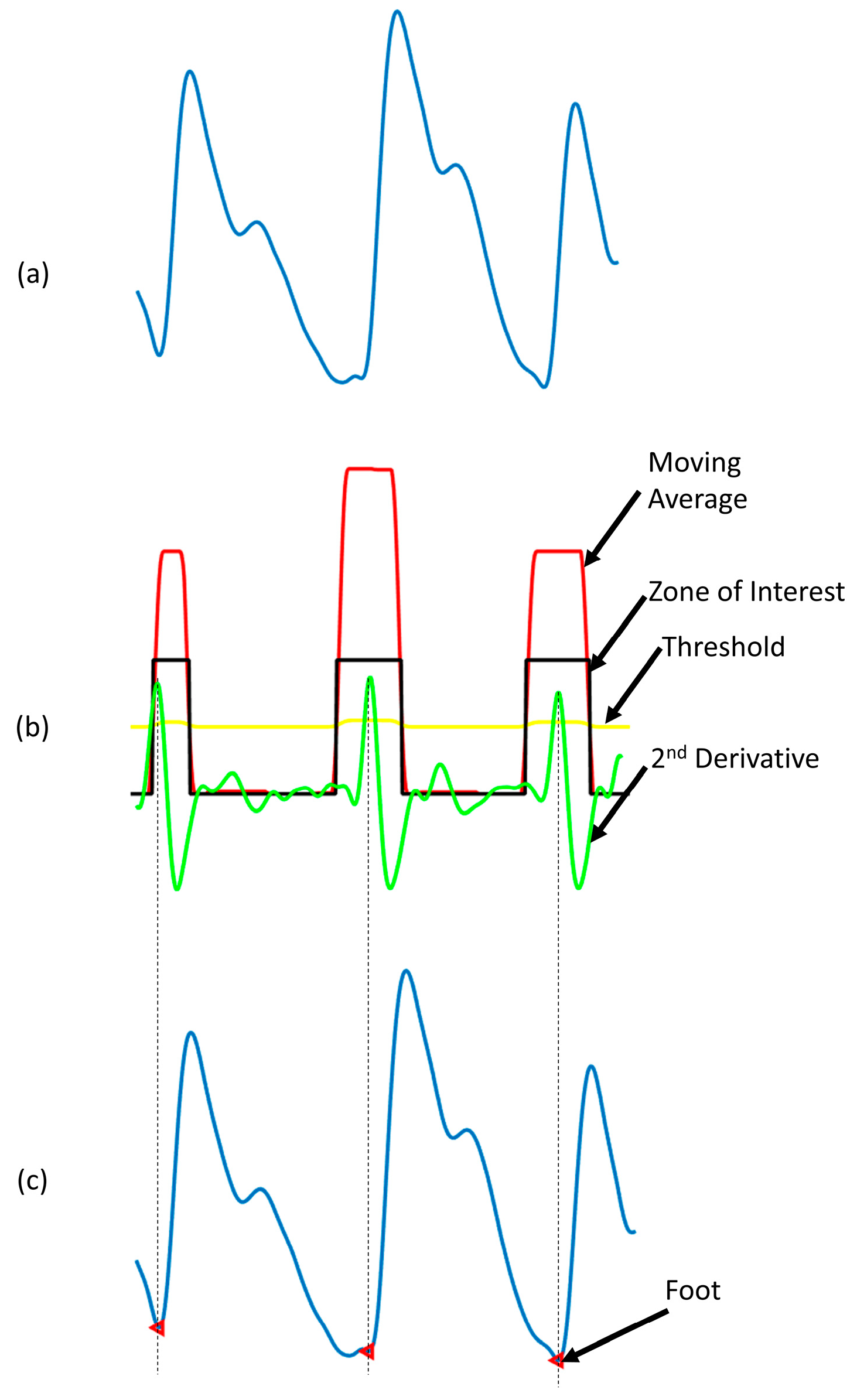
2.2.3. Baseline Correction
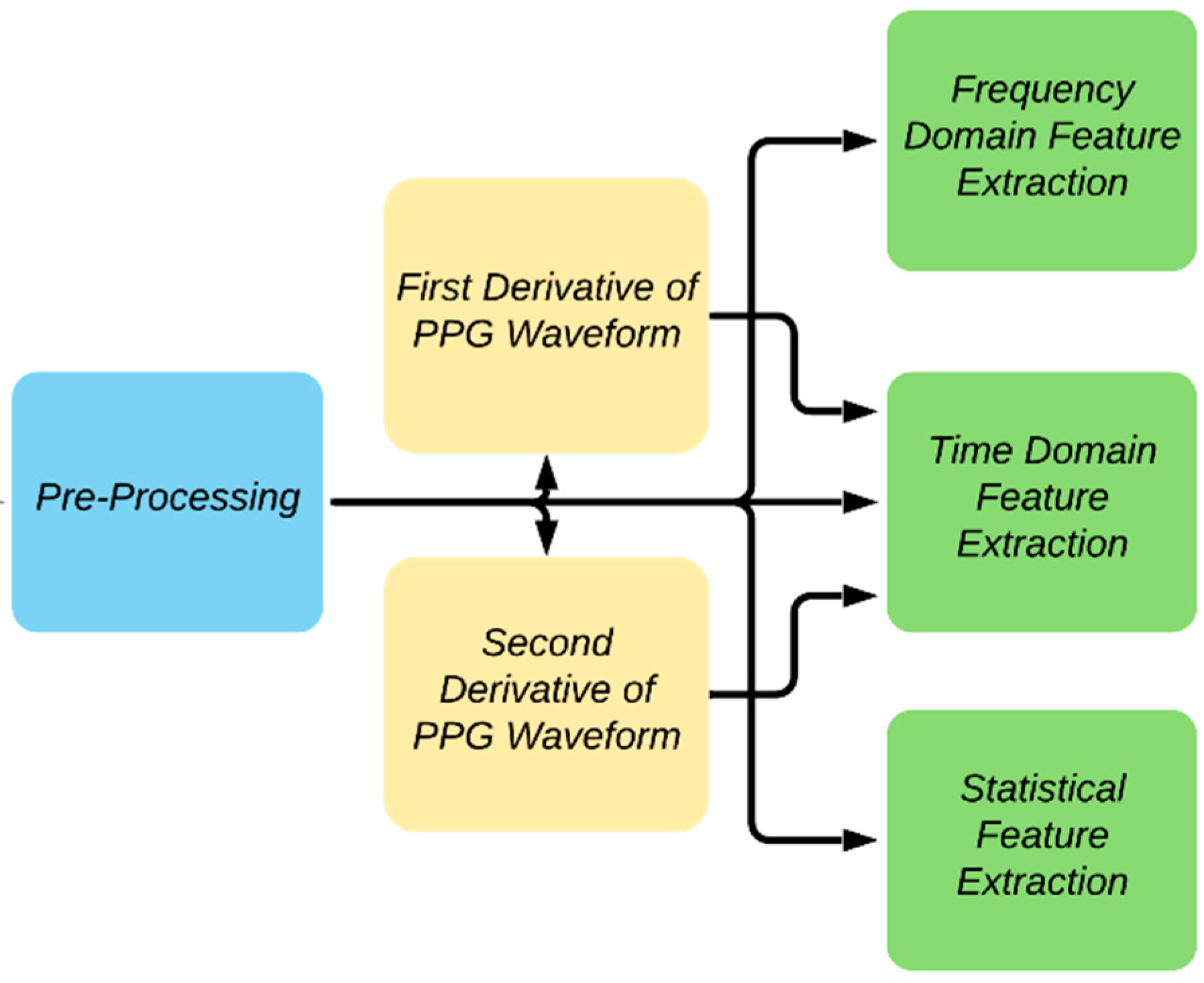
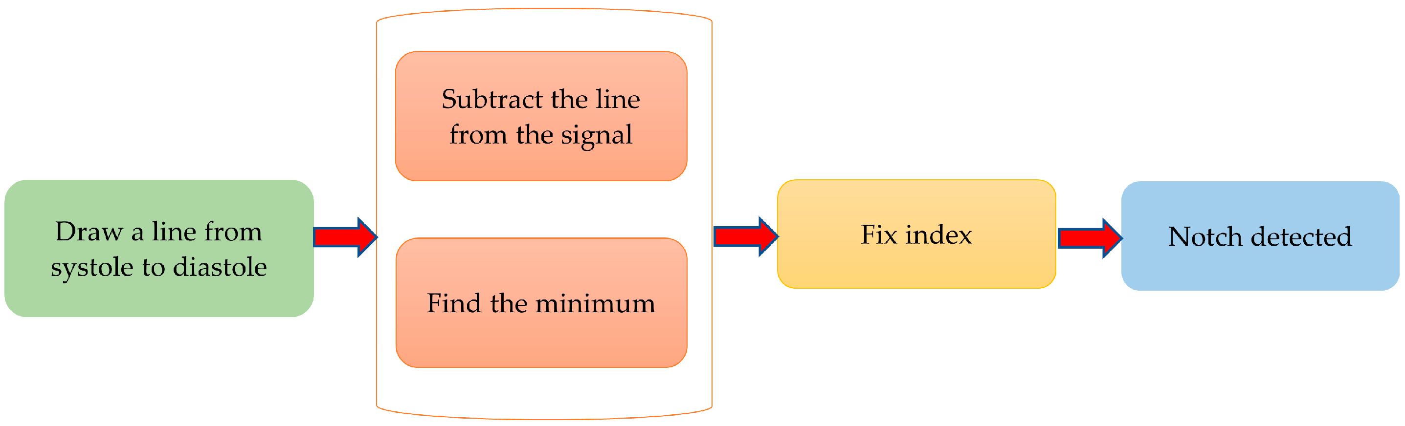
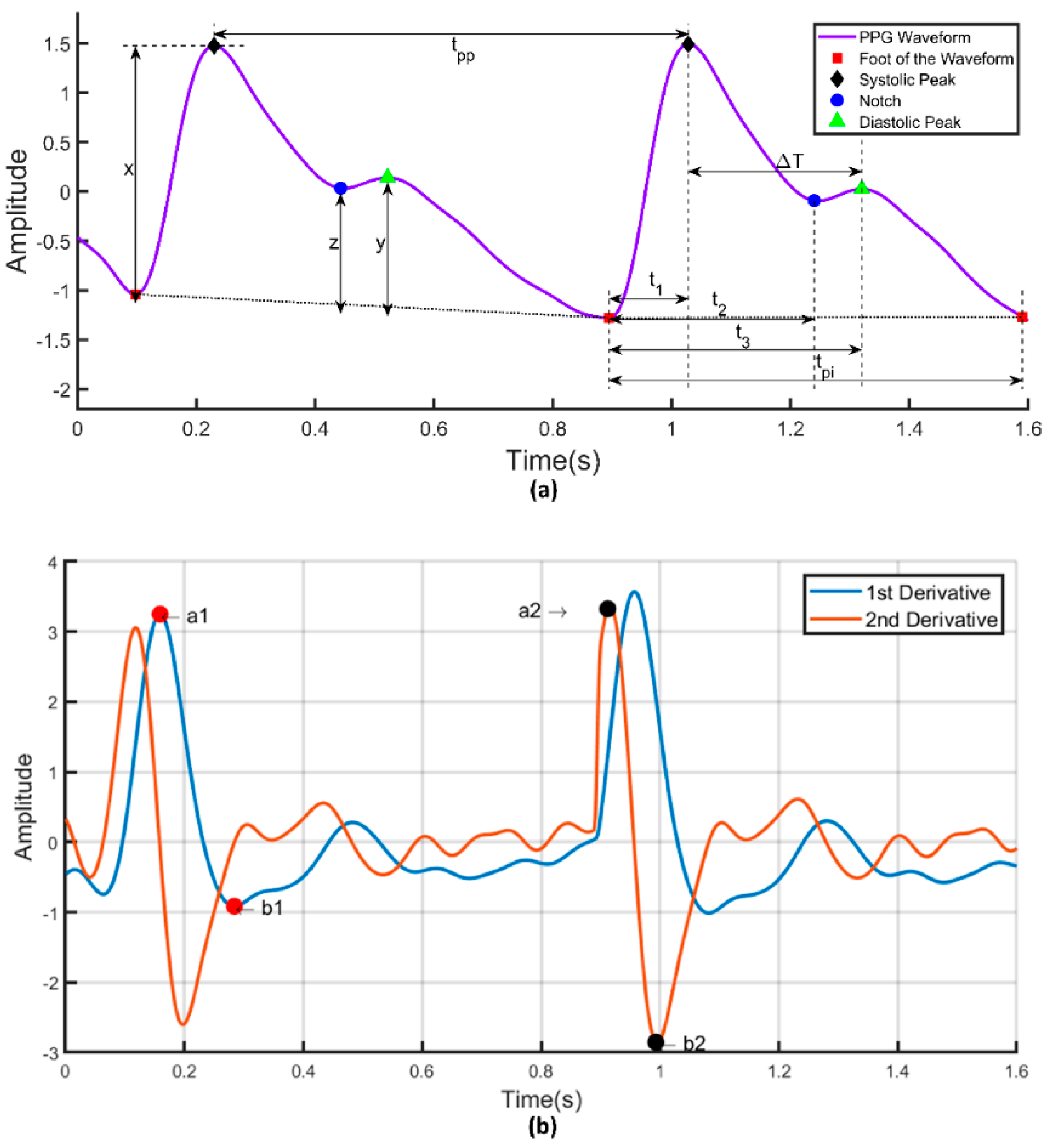
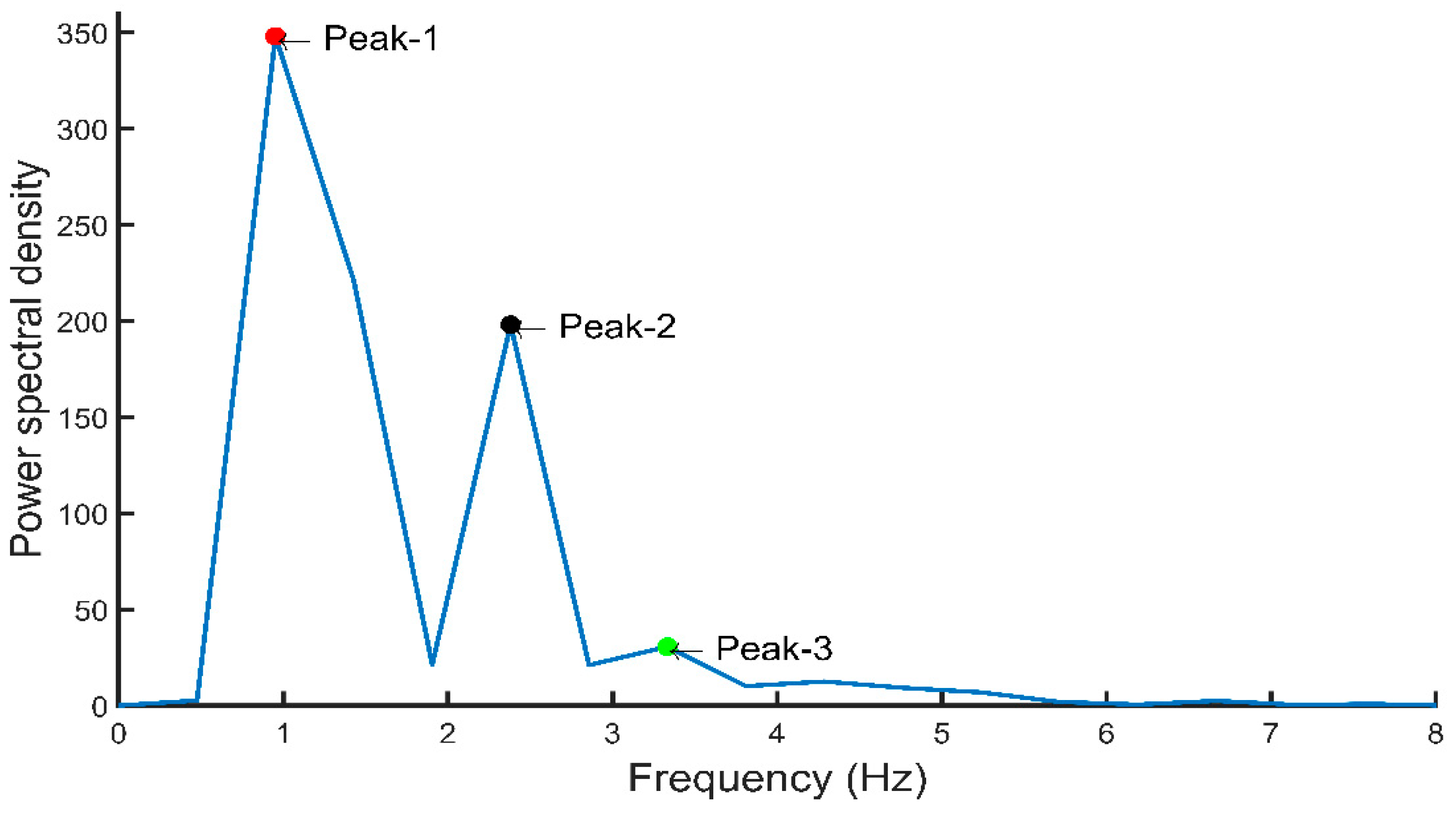
2.3. Feature Extraction
2.4. Feature Selection
2.5. Machine Learning (ML) Algorithms
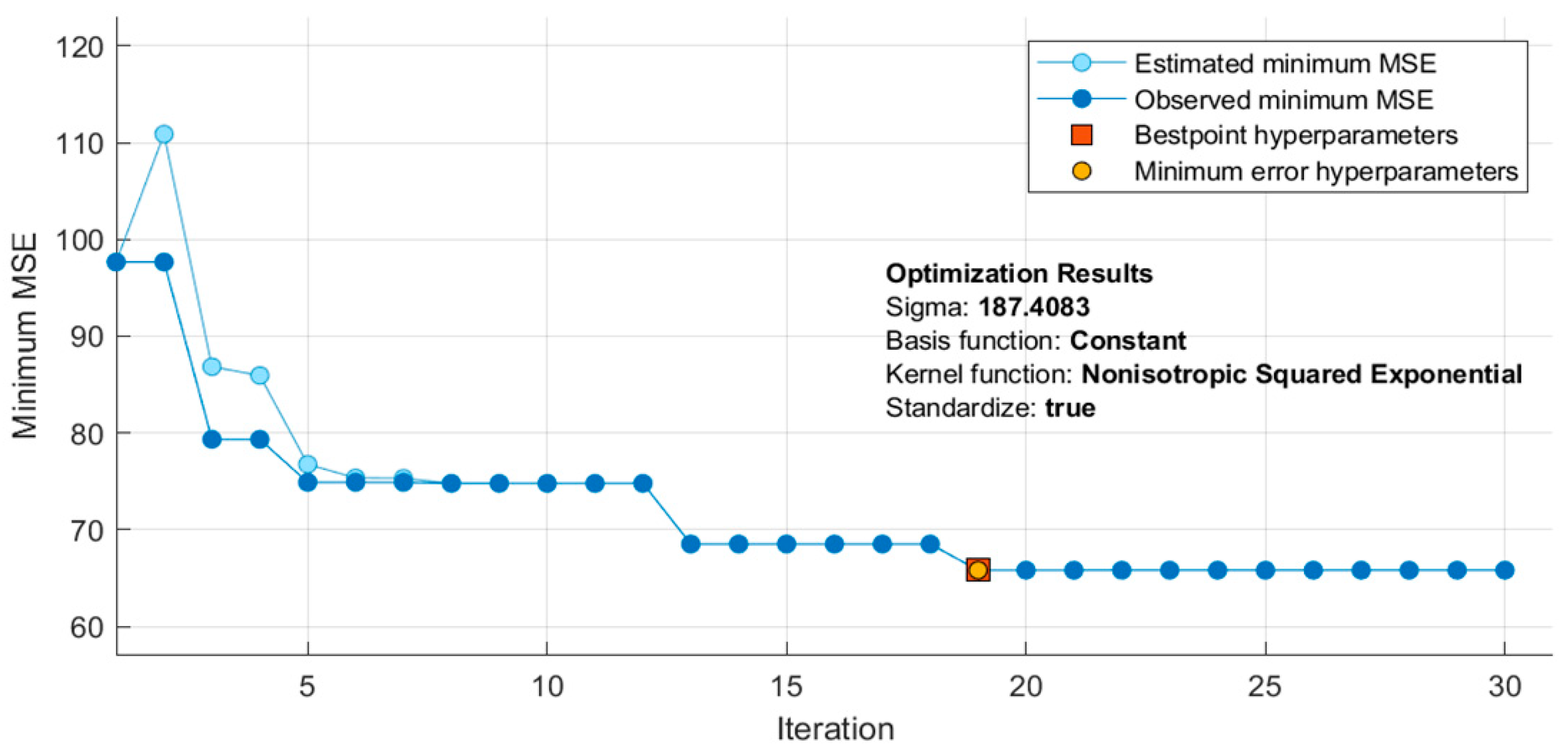
2.6. Hyper-Parameters Optimization of the Best Performing Algorithm
2.7. Evaluation Criteria
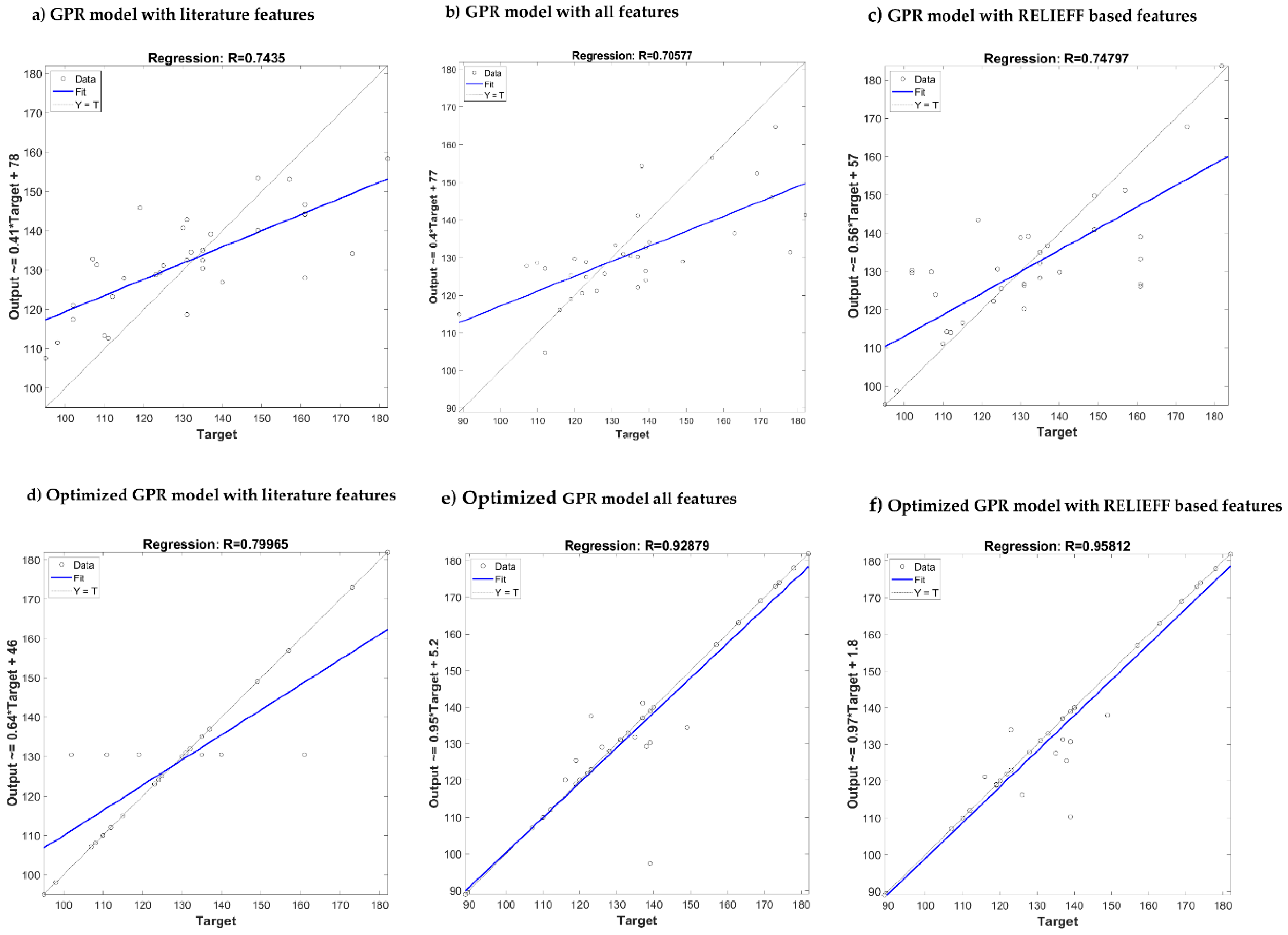
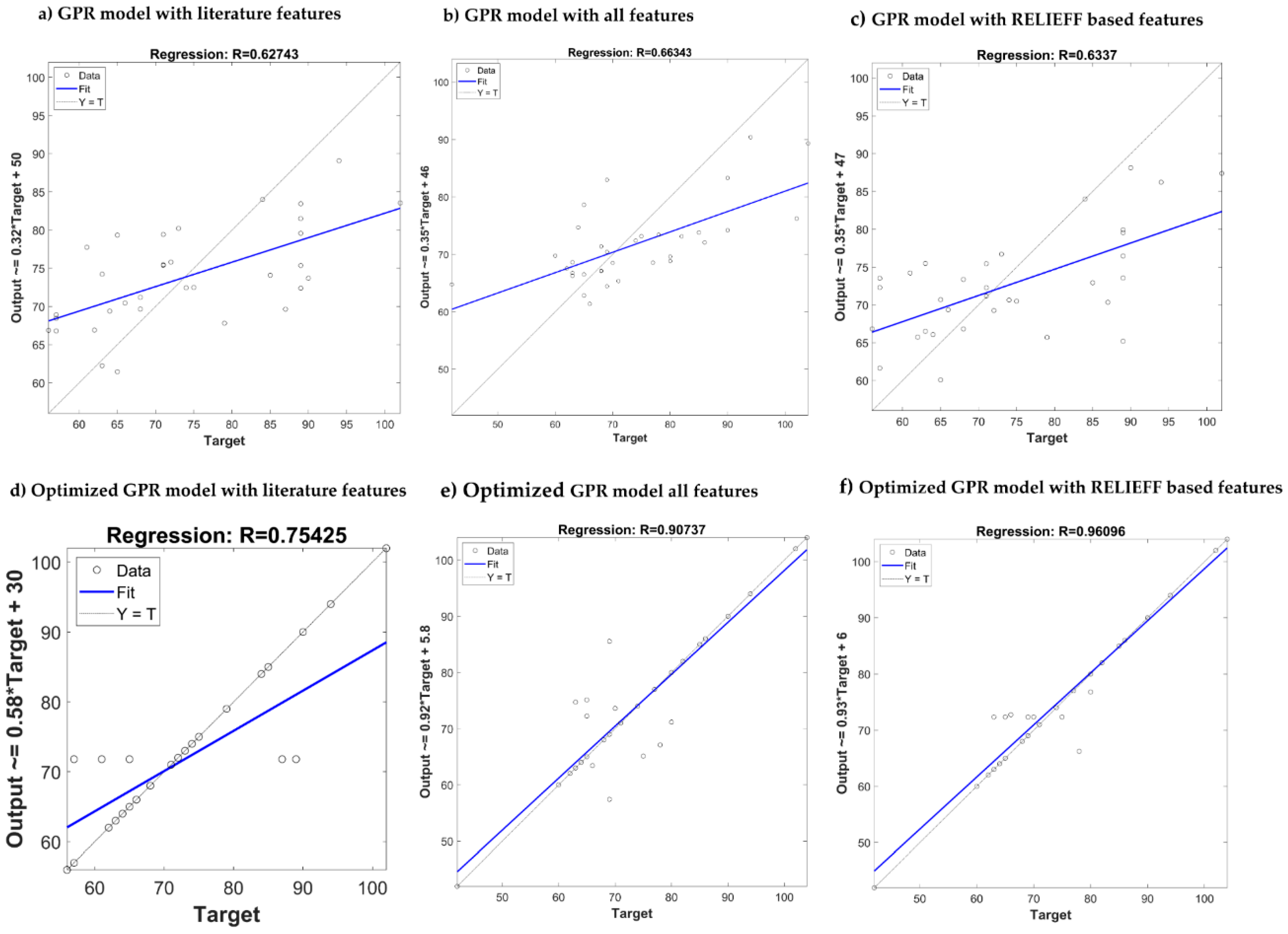
3. Results and Discussion
4. Conclusions
Author Contributions
Funding
Conflicts of Interest
References
- Why is Blood Pressure Important. Available online: http://www.bloodpressureuk.org/microsites/u40/Home/facts/Whyitmatters/ (accessed on 23 January 2020).
- 24-Hour Ambulatory Blood Pressure Monitoring (ABPM). Available online: http://www.bloodpressureuk.org/BloodPressureandyou/Medicaltests/24-hourtest/ (accessed on 23 January 2020).
- Chowdhury, M.E.; Alzoubi, K.; Khandakar, A.; Khallifa, R.; Abouhasera, R.; Koubaa, S.; Ahmed, R.; Hasan, A. Wearable real-time heart attack detection and warning system to reduce road accidents. Sensors 2019, 19, 2780. [Google Scholar] [CrossRef]
- Chowdhury, M.E.; Khandakar, A.; Alzoubi, K.; Mansoor, S.; Tahir, A.M.; Reaz, M.B.I.; Al-Emadi, N. Real-Time Smart-Digital Stethoscope System for Heart Diseases Monitoring. Sensors 2019, 19, 2781. [Google Scholar] [CrossRef] [PubMed]
- Lee, H.; Kim, E.; Lee, Y.; Kim, H.; Lee, J.; Kim, M.; Yoo, H.-J.; Yoo, S. Toward all-day wearable health monitoring: An ultralow-power, reflective organic pulse oximetry sensing patch. Sci. Adv. 2018, 4, eaas9530. [Google Scholar] [CrossRef] [PubMed]
- Chandrasekhar, A.; Kim, C.-S.; Naji, M.; Natarajan, K.; Hahn, J.-O.; Mukkamala, R. Smartphone-based blood pressure monitoring via the oscillometric finger-pressing method. Sci. Transl. Med. 2018, 10, eaap8674. [Google Scholar] [CrossRef] [PubMed]
- Liang, Y.; Chen, Z.; Ward, R.; Elgendi, M. Photoplethysmography and deep learning: Enhancing hypertension risk stratification. Biosensors 2018, 8, 101. [Google Scholar] [CrossRef]
- Elgendi, M.; Fletcher, R.; Liang, Y.; Howard, N.; Lovell, N.H.; Abbott, D.; Lim, K.; Ward, R. The use of photoplethysmography for assessing hypertension. NPJ Digit. Med. 2019, 2, 1–11. [Google Scholar] [CrossRef]
- Elgendi, M. On the analysis of fingertip photoplethysmogram signals. Curr. Cardiol. Rev. 2012, 8, 14–25. [Google Scholar] [CrossRef]
- Allen, J. Photoplethysmography and its application in clinical physiological measurement. Physiol. Meas. 2007, 28, R1. [Google Scholar] [CrossRef]
- Otsuka, T.; Kawada, T.; Katsumata, M.; Ibuki, C. Utility of second derivative of the finger photoplethysmogram for the estimation of the risk of coronary heart disease in the general population. Circ. J. 2006, 70, 304–310. [Google Scholar] [CrossRef]
- Millasseau, S.C.; Kelly, R.; Ritter, J.; Chowienczyk, P. Determination of age-related increases in large artery stiffness by digital pulse contour analysis. Clin. Sci. 2002, 103, 371–377. [Google Scholar] [CrossRef]
- Zheng, Y.; Poon, C.C.; Yan, B.P.; Lau, J.Y. Pulse arrival time based cuff-less and 24-H wearable blood pressure monitoring and its diagnostic value in hypertension. J. Med. Syst. 2016, 40, 195. [Google Scholar] [CrossRef] [PubMed]
- Lee, C.; Shin, H.S.; Lee, M. Relations between ac-dc components and optical path length in photoplethysmography. J. Biomed. Opt. 2011, 16, 077012. [Google Scholar] [CrossRef] [PubMed]
- Utami, N.; Setiawan, A.W.; Zakaria, H.; Mengko, T.R.; Mengko, R. Extracting blood flow parameters from Photoplethysmograph signals: A review. In Proceedings of the 2013 3rd International Conference on Instrumentation, Communications, Information Technology and Biomedical Engineering (ICICI-BME), Bandung, Indonesia, 7–8 November 2013; pp. 403–407. [Google Scholar]
- Bashkatov, A.; Genina, E.; Kochubey, V.; Tuchin, V. Optical properties of human skin, subcutaneous and mucous tissues in the wavelength range from 400 to 2000 nm. J. Phys. D Appl. Phys. 2005, 38, 2543. [Google Scholar] [CrossRef]
- Van Gastel, M.; Stuijk, S.; de Haan, G. New principle for measuring arterial blood oxygenation, enabling motion-robust remote monitoring. Sci. Rep. 2016, 6, 1–16. [Google Scholar] [CrossRef] [PubMed]
- Liang, Y.; Elgendi, M.; Chen, Z.; Ward, R. An optimal filter for short photoplethysmogram signals. Sci. Data 2018, 5, 180076. [Google Scholar] [CrossRef] [PubMed]
- Waugh, W.; Allen, J.; Wightman, J.; Sims, A.J.; Beale, T.A. Novel signal noise reduction method through cluster analysis, applied to photoplethysmography. Comput. Math. Methods Med. 2018, 2018, 6812404. [Google Scholar] [CrossRef]
- Lee, H.; Chung, H.; Ko, H.; Lee, J. Wearable multichannel photoplethysmography framework for heart rate monitoring during intensive exercise. IEEE Sens. J. 2018, 18, 2983–2993. [Google Scholar] [CrossRef]
- Xing, X.; Ma, Z.; Zhang, M.; Zhou, Y.; Dong, W.; Song, M. An Unobtrusive and Calibration-free Blood pressure estimation Method using photoplethysmography and Biometrics. Sci. Rep. 2019, 9, 1–8. [Google Scholar] [CrossRef]
- Rundo, F.; Ortis, A.; Battiato, S.; Conoci, S. Advanced bio-inspired system for noninvasive cuff-less blood pressure estimation from physiological signal analysis. Computation 2018, 6, 46. [Google Scholar] [CrossRef]
- Kim, J.Y.; Cho, B.H.; Im, S.M.; Jeon, M.J.; Kim, I.Y.; Kim, S.I. Comparative study on artificial neural network with multiple regressions for continuous estimation of blood pressure. In Proceedings of the 2005 IEEE Engineering in Medicine and Biology 27th Annual Conference, Shanghai, China, 17–18 January 2006; pp. 6942–6945. [Google Scholar]
- Kachuee, M.; Kiani, M.M.; Mohammadzade, H.; Shabany, M. Cuff-less high-accuracy calibration-free blood pressure estimation using pulse transit time. In Proceedings of the 2015 IEEE International Symposium on Circuits and Systems (ISCAS), Lisbon, Portugal, 24–27 May 2015; pp. 1006–1009. [Google Scholar]
- Cattivelli, F.S.; Garudadri, H. Noninvasive cuffless estimation of blood pressure from pulse arrival time and heart rate with adaptive calibration. In Proceedings of the 2009 Sixth International Workshop on Wearable and Implantable Body Sensor Networks, Berkeley, CA, USA, 3–5 June 2009; pp. 114–119. [Google Scholar]
- Xing, X.; Sun, M. Optical blood pressure estimation with photoplethysmography and FFT-based neural networks. Biomed. Opt. Express 2016, 7, 3007–3020. [Google Scholar] [CrossRef]
- Zhang, Y.; Feng, Z. A SVM method for continuous blood pressure estimation from a PPG signal. In Proceedings of the 9th International Conference on Machine Learning and Computing, Singapore, 24–26 February 2017; pp. 128–132. [Google Scholar]
- Su, P.; Ding, X.-R.; Zhang, Y.-T.; Liu, J.; Miao, F.; Zhao, N. Long-term blood pressure prediction with deep recurrent neural networks. In Proceedings of the 2018 IEEE EMBS International Conference on Biomedical & Health Informatics (BHI), Las Vegas, NV, USA, 4–7 March 2018; pp. 323–328. [Google Scholar]
- Gotlibovych, I.; Crawford, S.; Goyal, D.; Liu, J.; Kerem, Y.; Benaron, D.; Yilmaz, D.; Marcus, G.; Li, Y. End-to-end deep learning from raw sensor data: Atrial fibrillation detection using wearables. arXiv 2018, arXiv:1807.10707. [Google Scholar]
- Slapničar, G.; Mlakar, N.; Luštrek, M. Blood Pressure Estimation from Photoplethysmogram Using a Spectro-Temporal Deep Neural Network. Sensors 2019, 19, 3420. [Google Scholar] [CrossRef] [PubMed]
- Liang, G.L.Y.; Chen, Z.; Elgendi, M. PPG-BP Database. 2018. Available online: https://figshare.com/articles/PPG-BP_Database_zip/5459299/ (accessed on 21 October 2019).
- Liang, Y.; Chen, Z.; Liu, G.; Elgendi, M. A new, short-recorded photoplethysmogram dataset for blood pressure monitoring in China. Sci. Data 2018, 5, 180020. [Google Scholar] [CrossRef] [PubMed]
- Liang, Y.; Chen, Z.; Ward, R.; Elgendi, M. Hypertension assessment via ECG and PPG signals: An evaluation using MIMIC database. Diagnostics 2018, 8, 65. [Google Scholar] [CrossRef]
- Liang, Y.; Chen, Z.; Ward, R.; Elgendi, M. Hypertension assessment using photoplethysmography: A risk stratification approach. J. Clin. Med. 2019, 8, 12. [Google Scholar] [CrossRef]
- Ferdinando, H.; Huotari, M.; Myllylä, T. Photoplethysmography signal analysis to assess obesity, age group and hypertension. In Proceedings of the 2019 41st Annual International Conference of the IEEE Engineering in Medicine and Biology Society (EMBC), Berlin, Germany, 23–27 July 2019; pp. 5572–5575. [Google Scholar]
- Kavsaoğlu, A.R.; Polat, K.; Hariharan, M. Non-invasive prediction of hemoglobin level using machine learning techniques with the PPG signal’s characteristics features. Appl. Soft Comput. 2015, 37, 983–991. [Google Scholar] [CrossRef]
- Elgendi, M.; Norton, I.; Brearley, M.; Abbott, D.; Schuurmans, D. Detection of a and b waves in the acceleration photoplethysmogram. Biomed. Eng. Online 2014, 13, 139. [Google Scholar] [CrossRef]
- Kavsaoğlu, A.R.; Polat, K.; Bozkurt, M.R. A novel feature ranking algorithm for biometric recognition with PPG signals. Comput. Biol. Med. 2014, 49, 1–14. [Google Scholar] [CrossRef]
- Mahbub, Z.B.; Rabbani, K. Frequency domain analysis to identify neurological disorders from evoked EMG responses. J. Biol. Phys. 2007, 33, 99–108. [Google Scholar] [CrossRef]
- Yang, S.; Zhang, Y.; Cho, S.-Y.; Morgan, S.P.; Correia, R.; Wen, L. Cuff-less blood pressure measurement using fingertip photoplethysmogram signals and physiological characteristics. In Proceedings of the Optics in Health Care and Biomedical Optics VIII, Beijing, China, 23 October 2018; p. 1082036. [Google Scholar]
- Chatterjee, A.; Roy, U.K. PPG Based Heart Rate Algorithm Improvement with Butterworth IIR Filter and Savitzky-Golay FIR Filter. In Proceedings of the 2018 2nd International Conference on Electronics, Materials Engineering & Nano-Technology (IEMENTech), Kolkata, India, 4–5 May 2018; pp. 1–6. [Google Scholar]
- Sun, S.; Peeters, W.H.; Bezemer, R.; Long, X.; Paulussen, I.; Aarts, R.M.; Noordergraaf, G.J. Finger and forehead photoplethysmography-derived pulse-pressure variation and the benefits of baseline correction. J. Clin. Monit. Comput. 2019, 33, 65–75. [Google Scholar] [CrossRef]
- Maxwell, J.C. A Treatise on Electricity and Magnetism; Clarendon Press: Oxford, UK, 1881; Volume 1. [Google Scholar]
- McDuff, D.; Gontarek, S.; Picard, R.W. Remote detection of photoplethysmographic systolic and diastolic peaks using a digital camera. IEEE Trans. Biomed. Eng. 2014, 61, 2948–2954. [Google Scholar] [CrossRef] [PubMed]
- Laurin, A. BP_Annotate. Available online: https://www.mathworks.com/matlabcentral/fileexchange/60172-bp_annotate/ (accessed on 21 November 2019).
- Pan, J.; Tompkins, W.J. A real-time QRS detection algorithm. IEEE Trans. Biomed. Eng. 1985, 32, 230–236. [Google Scholar] [CrossRef] [PubMed]
- Sun, J.; Reisner, A.; Mark, R. A signal abnormality index for arterial blood pressure waveforms. In Proceedings of the 2006 Computers in Cardiology, Valencia, Spain, 17–20 September 2006; pp. 13–16. [Google Scholar]
- Monte-Moreno, E. Non-invasive estimate of blood glucose and blood pressure from a photoplethysmograph by means of machine learning techniques. Artif. Intell. Med. 2011, 53, 127–138. [Google Scholar] [CrossRef] [PubMed]
- Kurylyak, Y.; Lamonaca, F.; Grimaldi, D. A Neural Network-based method for continuous blood pressure estimation from a PPG signal. In Proceedings of the 2013 IEEE International Instrumentation and Measurement Technology Conference (I2MTC), Minneapolis, MN, USA, 6–9 May 2013; pp. 280–283. [Google Scholar]
- Kira, K.; Rendell, L.A. The feature selection problem: Traditional methods and a new algorithm. Aaai 1992, 2, 129–134. [Google Scholar]
- Kononenko, I.; Šimec, E.; Robnik-Šikonja, M. Overcoming the myopia of inductive learning algorithms with RELIEFF. Appl. Intell. 1997, 7, 39–55. [Google Scholar] [CrossRef]
- Roffo, G. Ranking to learn and learning to rank: On the role of ranking in pattern recognition applications. arXiv 2017, arXiv:1706.05933. [Google Scholar]
- Ding, C.; Peng, H. Minimum redundancy feature selection from microarray gene expression data. J. Bioinform. Comput. Biol. 2005, 3, 185–205. [Google Scholar] [CrossRef]
- Darbellay, G.A.; Vajda, I. Estimation of the information by an adaptive partitioning of the observation space. IEEE Trans. Inf. Theory 1999, 45, 1315–1321. [Google Scholar] [CrossRef]
- Khandakar, A.; Chowdhury, M.E.H.; Kazi, M.K.; Benhmed, K.; Touati, F.; Al-Hitmi, M.; Antonio, S.P., Jr. Gonzales. Machine learning based photovoltaics (PV) power prediction using different environmental parameters of Qatar. Energies 2019, 12, 2782. [Google Scholar] [CrossRef]
- Sit, H. Quick Start to Gaussian Process Regression. Available online: https://towardsdatascience.com/quick-start-to-gaussian-process-regression-36d838810319/ (accessed on 23 January 2020).
- Ensemble Algorithms. Available online: https://www.mathworks.com/help/stats/ensemble-algorithms.html/ (accessed on 23 January 2020).
- Filion, A. (1994–2020). Applied Machine Learning, Part 3: Hyperparameter Optimization. Available online: https://www.mathworks.com/videos/applied-machine-learning-part-3-hyperparameter-optimization-1547849445386.html/ (accessed on 23 January 2020).
- Zadi, A.S.; Alex, R.; Zhang, R.; Watenpaugh, D.E.; Behbehani, K. Arterial blood pressure feature estimation using photoplethysmography. Comput. Biol. Med. 2018, 102, 104–111. [Google Scholar] [CrossRef]
- Stergiou, G.S.; Alpert, B.; Mieke, S.; Asmar, R.; Atkins, N.; Eckert, S.; Frick, G.; Friedman, B. A universal standard for the validation of blood pressure measuring devices: Association for the Advancement of Medical Instrumentation/European Society of Hypertension/International Organization for Standardization (AAMI/ESH/ISO) Collaboration Statement. Hypertension 2018, 71, 368–374. [Google Scholar] [CrossRef]
- Mousavi, S.S.; Firouzmand, M.; Charmi, M.; Hemmati, M.; Moghadam, M.; Ghorbani, Y. Blood pressure estimation from appropriate and inappropriate PPG signals using A whole-based method. Biomed. Signal Process. Control 2019, 47, 196–206. [Google Scholar] [CrossRef]
- Association for the Advancement of Medical Instrumentation. American National Standard. Manual, Electronic or Automated Sphygmomanometers; ANSI/AAMI SP10-2002/A1; Association for the Advancement of Medical Instrumentation: Arlington, VA, USA, 2003. [Google Scholar]
- O’brien, E.; Waeber, B.; Parati, G.; Staessen, J.; Myers, M.G. Blood pressure measuring devices: Recommendations of the European Society of Hypertension. BMJ 2001, 322, 531–536. [Google Scholar] [CrossRef]


| Physical Index | Numerical Data |
|---|---|
| Females | 115 (52%) |
| Age (years) | 57 ± 15 |
| Height (cm) | 161 ± 8 |
| Weight (kg) | 60 ± 11 |
| Body Mass Index (kg/m2) | 23 ± 4 |
| Systolic Blood Pressure (mmHg) | 127 ± 20 |
| Diastolic Blood Pressure (mmHg) | 71 ± 11 |
| Heart Rate (beats/min) | 73 ± 10 |
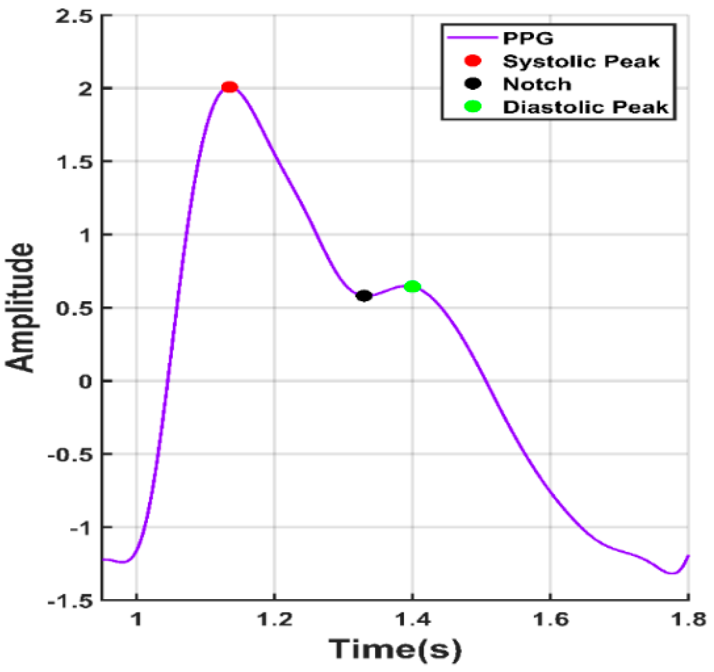
| Feature | Definition |
|---|---|
| 1. Systolic Peak | The amplitude of (‘x’) from PPG waveform |
| 2. Diastolic Peak | The amplitude of (‘y’) from PPG waveform |
| 3. Height of Notch | The amplitude of (‘z’) from PPG waveform |
| 4. Systolic Peak Time | The time interval from the foot of the waveform to the systolic peak (‘t1’) |
| 5. Diastolic Peak Time | The time interval from the foot of the waveform to the height of notch (‘t2’) |
| 6. Height of Notch Time | The time interval from the foot of the waveform to the diastolic peak (‘t3’) |
| 7. ∆T | The time interval from systolic peak time to diastolic peak time |
| 8. Pulse Interval | The distance between the beginning and the end of the PPG waveform (‘tpi’) |
| 9. Peak-to-Peak Interval | The distance between two consecutive systolic peaks (tpp) |
| 10. Pulse Width | The half-height of the systolic peak |
| 11. Inflection Point Area | The waveform is first split into two parts at the notch point. The area of the first part is A1 and the area of the second part is A2. The ratio of A1 and A2 is the inflection point area (‘A1/A2 ’) |
| 12. Augmentation Index | The ratio of diastolic and systolic peak amplitude (‘y/x’) |
| 13. Alternative Augmentation Index | The difference between systolic and diastolic peak amplitude divided by systolic peak amplitude (‘(x-y)/x’) |
| 14. Systolic Peak Output Curve | The ratio of systolic peak time to systolic peak amplitude (‘t1/x’) |
| 15. Diastolic Peak Downward Curve | The ratio of diastolic peak amplitude to the differences between pulse interval and height of notch time (‘y/ tpi-t3’) |
| 16. t1/tpp | The ratio of systolic peak time to the peak-to-peak interval of the PPG waveform |
| 17. t2/tpp | The ratio of notch time to the peak-to-peak interval of the PPG waveform |
| 18. t3/tpp | The ratio of diastolic peak time to the peak-to-peak interval of the PPG waveform |
| 19. ∆T/tpp | The ratio of ∆T to the peak-to-peak interval of the PPG waveform |
| 20. z/x | The ratio of the height of notch to the systolic peak amplitude |
| 21. t2/z | The ratio of the notch time to the height of notch |
| 22. t3/y | The ratio of the diastolic peak time to the diastolic peak amplitude |
| 23. x/(tpi-t1) | The ratio of systolic peak amplitude to the difference between pulse interval and systolic peak time |
| 24. z/(tpi-t2) | The ratio of the height of notch to the difference between pulse interval and notch time |
| Feature | Definition |
|---|---|
| 25. Width (25%) | The width of the waveform at 25% amplitude of systolic amplitude |
| 26. Width (75%) | The width of the waveform at 75% amplitude of systolic amplitude |
| 27. Width (25%)/t1 | The ratio of pulse width at 25% of systolic amplitude to systolic peak time |
| 28. Width (25%)/t2 | The ratio of pulse width at 25% of systolic amplitude to notch time |
| 29. Width (25%)/t3 | The ratio of pulse width at 25% of systolic amplitude to diastolic peak time |
| 30. Width (25%)/∆T | The ratio of pulse width at 25% of systolic amplitude to ∆T |
| 31. Width (25%)/tpi | The ratio of pulse width at 25% of systolic amplitude to pulse interval |
| 32. Width (50%)/t1 | The ratio of pulse width at 50% of systolic amplitude to systolic peak time |
| 33. Width (50%)/t2 | The ratio of pulse width at 50% of systolic amplitude to notch time |
| 34. Width (50%)/t3 | The ratio of pulse width at 50% of systolic amplitude to diastolic peak time |
| 35. Width (50%)/∆T | The ratio of pulse width at 50% of systolic amplitude to ∆T |
| 36. Width (50%)/tpi | The ratio of pulse width at 50% of systolic amplitude to pulse interval |
| 37. Width (75%)/t1 | The ratio of pulse width at 75% of systolic amplitude to systolic peak time |
| 38. Width (75%)/t2 | The ratio of pulse width at 75% of systolic amplitude to notch time |
| 39. Width (75%)/t3 | The ratio of pulse width at 75% of systolic amplitude to diastolic peak time |
| 40. Width (75%)/∆T | The ratio of pulse width at 75% of systolic amplitude to ∆T |
| 41. Width (75%)/tpi | The ratio of pulse width at 75% of systolic amplitude to pulse interval |
| Feature | Definition |
|---|---|
| 42. a1 | The first maximum peak from the first derivative of the PPG waveform |
| 43. ta1 | The time interval from the foot of the PPG waveform to the time at which a1 occurred |
| 44. a2 | The first maximum peak from the second derivative of the PPG waveform after a1 |
| 45. ta2 | The time interval from the foot of the PPG waveform to the time at which a2 occurred |
| 46. b1 | The first minimum peak from the first derivative of the PPG waveform after a1 |
| 47. tb1 | The time interval from the foot of the PPG waveform to the time at which b1 occurred |
| 48. b2 | The first minimum peak from the second derivative of the PPG waveform after a2 |
| 49. tb2 | The time interval from the foot of the PPG waveform to the time at which b2 occurred |
| 50. b2/a2 | The ratio of b2 to a2 |
| 51. b1/a1 | The ratio of first minimum peak of the first derivative after a1 to first maximum peak of the first derivative |
| 52. ta1/tpp | The ratio of ta1 to the peak-to-peak interval of the PPG waveform |
| 53. tb1/tpp | The ratio of tb1 to the peak-to-peak interval of the PPG waveform |
| 54. tb2/tpp | The ratio of tb2 to the peak-to-peak interval of the PPG waveform |
| 55. ta2/tpp | The ratio of ta2 to the peak-to-peak interval of the PPG waveform |
| 56. (ta1–ta2)/tpp | The ratio of the difference between ta1 and ta2 to the peak-to-peak interval of the PPG waveform |
| 57. (tb1–tb2)/tpp | The ratio of the difference between tb1 and tb2 to the peak-to-peak interval of the PPG waveform |
| Feature | Definition |
|---|---|
| 58. Height/∆T | It is known as stiffness index |
| 59. Weight/∆T | The ratio of weight to ∆T |
| 60. BMI/∆T | The ratio of BMI to ∆T |
| 61. Height/t1 | The ratio of height to the systolic peak time |
| 62. Weight/t1 | The ratio of weight to the systolic peak time |
| 63. BMI/t1 | The ratio of BMI to the systolic peak time |
| 64. Height/t2 | The ratio of height to the notch time |
| 65. Weight/t2 | The ratio of weight to the notch time |
| 66. BMI/t2 | The ratio of BMI to the notch time |
| 67. Height/t3 | The ratio of height to the diastolic peak time |
| 68. Weight/t3 | The ratio of weight to the diastolic peak time |
| 69. BMI/t3 | The ratio of BMI to the diastolic peak time |
| 70. Height/tpi | The ratio of height to the pulse interval |
| 71. Weight/tpi | The ratio of weight to the pulse interval |
| 72. BMI/tpi | The ratio of BMI to the pulse interval |
| 73. Height/tpp | The ratio of height to the peak-to-peak interval |
| 74. Weight/tpp | The ratio of weight to the peak-to-peak interval |
| 75. BMI/tpp | The ratio of BMI to the peak-to-peak interval |
| Feature | Definition |
|---|---|
| 76. Peak-1 | The amplitude of the first peak from the fast Fourier transform of the PPG signal |
| 77. Peak-2 | The amplitude of the second peak from the fast Fourier transform of the PPG signal |
| 78. Peak-3 | The amplitude of the third peak from the fast Fourier transform of the PPG signal |
| 79. Freq-1 | The frequency at which the first peak from the fast Fourier transform of the PPG signal occurred |
| 80. Freq-2 | The frequency at which the second peak from the fast Fourier transform of the PPG signal occurred |
| 81. Freq-3 | The frequency at which the third peak from the fast Fourier transform of the PPG signal occurred |
| 82. A0–2 | Area under the curve from 0 to 2 Hz for the fast Fourier transform of the PPG signal |
| 83. A2–5 | Area under the curve from 2 to 5 Hz for the fast Fourier transform of the PPG signal |
| 84. A0–2/A2–5 | The ratio of the area under the curve from 0 to 2 Hz to the area under the curve from 2 to 5 Hz |
| 85. Peak-1/peak-2 | The ratio of the first peak to the second peak from the fast Fourier transform of the PPG signal |
| 86. Peak-1/peak-3 | The ratio of the first peak to the third peak from the fast Fourier transform of the PPG signal |
| 87. Freq-1/freq-2 | The ratio of the frequency at first peak to the frequency at second peak from the fast Fourier transform of the PPG signal |
| 88. Freq-1/freq-3 | The ratio of the frequency at first peak to the frequency at third peak from the fast Fourier transform of the PPG signal |
| 89. Maximum Frequency | The value of highest frequency in the signal spectrum |
| 90. Magnitude at Fmax | Signal magnitude at highest frequency X |
| 91. Ratio of signal energy | Ratio of signal energy between ) and the whole spectrum X |
| Feature | Definition | Equation |
|---|---|---|
| 92. Mean | Sum of all data divided by the number of entries | |
| 93. Median | Value that is in the middle of the ordered set of data | Odd numbers of entries: Median = middle data entry. Even numbers of entries: Median = adding the two numbers in the middle and dividing the result by two. |
| 94. Standard Deviation | Measure variability and consistency of the sample. | = |
| 95. Percentile | The data value at which the percent of the value in the data set are less than or equal to this value. | 25th = ()n |
| 75th = ()n | ||
| 96. Mean Absolute Deviation | Average distance between the mean and each data value. | MAD = |
| 97. Inter Quartile Range (IQR) | The measure of the middle 50% of data. | IQR = Q3–Q1 Q3: Third quartile, Q1: First quartile, Quartile: Dividing the data set into four equal portions. |
| 98. Skewness | The measure of the lack of symmetry from the mean of the dataset. | g1 = Y: Mean, s: Standard deviation, N: Number of data. |
| 99. Kurtosis | The pointedness of a peak in distribution curve, in other words it is the measure of sharpness of the peak of distribution curve. | K = Y: Mean, s: Standard deviation, N: Number of data. |
| 100. Shannon’s Entropy | Entropy measures the degree of randomness in a set of data, higher entropy indicates a greater randomness, and lower entropy indicates a lower randomness. | H(x) = − |
| 101. Spectral Entropy | The normalized Shannon’s entropy that is applied to the power spectrum density of the signal. | SEN = : Spectral power of the normalized frequency, N: Number of frequencies in binary |
| 102. Height | 103. Weight | 104. Gender | 105. Age | 106. BMI | 107. Heart rate |
| Feature Selection Algorithms Used | Systolic Blood Pressure | Diastolic Blood Pressure |
|---|---|---|
| RELIEFF | 105. Age, 106. Heart Rate, 103. Weight, 102. Height, 107. BMI, 83. A2–5, 63. BMI/t1, 71. Weight/tpi, 74. Weight/tpp, 62. Weight/t1, 75. BMI/tpp | 105. Age, 106. Heart Rate, 103. Weight, 102. Height, 107. BMI, 69. BMI/t3, 71. Weight/tpi, 6. t3, 72. BMI/tpi, 82. A0–2, |
| FSCMRMR | 105. Age, 97. Inter Quartile Range, 45. ta2, 64. Height/t2, 13. Alternative Augmentation Index, 98. Skewness, 101. Spectral Entropy, 87. Freq-1/Freq-2, 23. x/(tpi-t1), 32. Width (50%)/t1, 36. Width (50%)/tpi, 99. Kurtosis, 30. Width (25%)/∆T | 103. Weight, 22. t3/y, 106. Heart Rate, 40. Width (75%)/∆T, 77. Peak-2, 100. Shannon’s Entropy, 96. Mean Absolute Deviation, 90. Magnitude at Fmax, 38. Width (75%)/t2, 58. Height/∆T, 101. Spectral Entropy, 31. Width (25%)/tpi, 105. Age |
| CFS | 69. BMI/t3, 71. Weight/tpi, 74. Weight/tpp, 49. tb2, 59. Weight/∆T, 51. b1/a1, 46. b1, 47. tb1, 62. Weight/t1, 52. ta1/tpp, 66. BMI/t2, 67. Height/t3, 100. Shannon’s Entropy, 48. b2, 75. BMI/tpp | 69. BMI/t3, 71. Weight/tpi, 74. Weight/tpp, 49. tb2, 59. Weight/∆T, 51. b1/a1, 46. b1, 47. tb1, 62. Weight/t1, 52. ta1/tpp, 66. BMI/t2, 67. Height/t3, 100. Shannon’s Entropy, 48. b2, 75. BMI/tpp |
| Selection Criteria | Performance Criteria | Systolic Blood Pressure | Diastolic Blood Pressure | ||
|---|---|---|---|---|---|
| GPR | Ensemble Trees | GPR | Ensemble Trees | ||
| Features from the literature | MAE MSE RMSE R | 12.27 240.25 15.50 0.71 | 12.68 246.74 15.70 0.71 | 8.31 96.90 9.84 0.62 | 8.82 109.92 10.45 0.54 |
| All features (newly designed and from the literature) | MAE MSE RMSE R | 12.06 272.32 16.50 0.70 | 12.95 316.71 17.80 0.59 | 7.70 97.31 9.86 0.63 | 8.31 110.87 10.53 0.57 |
| ReliefF | MAE MSE RMSE R | 10.08 219.08 14.80 0.74 | 12.57 258.16 16.06 0.69 | 7.87 96.70 9.83 0.62 | 8.93 119.32 10.92 0.49 |
| FSCMRMR | MAE MSE RMSE R | 13.92 302.75 17.39 0.62 | 15.10 349.06 18.68 0.55 | 8.84 112.27 10.59 0.53 | 9.66 128.43 11.33 0.42 |
| CFS | MAE MSE RMSE R | 11.91 257.77 16.05 0.69 | 13.06 325.29 18.03 0.65 | 7.64 83.95 9.16 0.68 | 8.27 103.70 10.18 0.58 |
| Selection Criteria | Performance Criteria | Systolic Blood Pressure | Diastolic Blood Pressure | ||
|---|---|---|---|---|---|
| Optimized GPR | Optimized Ensemble Trees | Optimized GPR | Optimized Ensemble Trees | ||
| Features from the literature | MAE MSE RMSE R | 6.79 180.99 13.45 0.79 | 12.43 231.15 15.20 0.73 | 4.49 70.06 8.37 0.74 | 8.17 104.45 10.27 0.57 |
| All features (newly designed and from the literature) | MAE MSE RMSE R | 3.30 72.95 8.54 0.92 | 10.886 264.24 16.25 0.67 | 2.81 30.70 5.54 0.90 | 7.96 111.97 10.58 0.56 |
| ReliefF | MAE MSE RMSE R | 3.02 45.49 6.74 0.95 | 11.32 284.69 16.84 0.65 | 1.74 12.89 3.59 0.96 | 5.99 62.04 7.88 0.78 |
| FSCMRMR | MAE MSE RMSE R | 6.11 108.96 10.44 0.88 | 14.65 321.63 17.93 0.58 | 6.80 77.26 8.78 0.72 | 8.22 110.84 10.53 0.56 |
| CFS | MAE MSE RMSE R | 12.95 361.96 19.02 0.50 | 16.27 448.25 21.17 0.28 | 7.59 108.43 10.41 0.57 | 7.89 106.72 10.33 0.58 |
| Author | Method Used | Number of Subjects | Performance Criteria | Systolic Blood Pressure | Diastolic Blood Pressure |
|---|---|---|---|---|---|
| Kachuee et al. [24] | SVM | MIMIC II (1000 subjects) | MAE MSE RMSE R | 12.38 - - - | 6.34 - - - |
| Kim et al. [23] | Multiple nonlinear regression (MLP) | 180 recordings, 45 subjects | MAE MSE RMSE R | 5.67 - - - | - - - - |
| Kim et al. [23] | Artificial neural network (ANN) | 180 recordings, 45 subjects | MAE MSE RMSE R | 4.53 - - - | - - - - |
| Cattivelli et al. [25] | Proprietary algorithm | MIMIC database (34 recordings, 25 subjects) | MAE MSE RMSE R | - 70.05 - - | - 35.08 - - |
| Zhang et al. [27] | Support vector machine (SVM) | 7000 samples from 32 patients | MAE MSE RMSE R | 11.64 - - - | 7.62 - - - |
| Zhang et al. [27] | Neural network (nine input neurons) | 7000 samples from 32 patients | MAE MSE RMSE R | 11.89 - - - | 8.83 - - - |
| Zadi et al. [59] | Autoregressive moving average (ARMA) models | 15 subjects | MAE MSE RMSE R | - - 6.49 - | - - 4.33 - |
| Slapničar et al. [30] | Deep learning (spectro-temporal ResNet) | MIMIC III database (510 subjects) | MAE MSE RMSE R | 9.43 - - - | 6.88 - - - |
| Su et al. [28] * | Deep learning (long short-term memory (LSTM)) | 84 subjects | MAE MSE RMSE R | - - 3.73 - | - - 2.43 - |
| This work | Gaussian process regression (GPR) | 222 recordings, 126 subjects | MAE MSE RMSE R | 3.02 45.49 6.74 0.95 | 1.74 12.89 3.59 0.96 |
| MEAN (mmHg) | SD (mmHg) | Subject | ||
|---|---|---|---|---|
| AAMI [62] | BP | ≤5 | ≤8 | ≥85 |
| This paper | SBP | 3.02 | 9.29 | 126 |
| DBP | 1.74 | 5.54 | 126 |
| ≤5 mmHg | ≤10 mmHg | ≤15 mmHg | ||
|---|---|---|---|---|
| BHS [63] | Grade A Grade B Grade C | 60% 50% 40% | 85% 75% 65% | 95% 90% 85% |
| This paper | SBP DBP | 69% 77% | 76% 85% | 92% 92% |
© 2020 by the authors. Licensee MDPI, Basel, Switzerland. This article is an open access article distributed under the terms and conditions of the Creative Commons Attribution (CC BY) license (http://creativecommons.org/licenses/by/4.0/).
Share and Cite
Chowdhury, M.H.; Shuzan, M.N.I.; Chowdhury, M.E.H.; Mahbub, Z.B.; Uddin, M.M.; Khandakar, A.; Reaz, M.B.I. Estimating Blood Pressure from the Photoplethysmogram Signal and Demographic Features Using Machine Learning Techniques. Sensors 2020, 20, 3127. https://doi.org/10.3390/s20113127
Chowdhury MH, Shuzan MNI, Chowdhury MEH, Mahbub ZB, Uddin MM, Khandakar A, Reaz MBI. Estimating Blood Pressure from the Photoplethysmogram Signal and Demographic Features Using Machine Learning Techniques. Sensors. 2020; 20(11):3127. https://doi.org/10.3390/s20113127
Chicago/Turabian StyleChowdhury, Moajjem Hossain, Md Nazmul Islam Shuzan, Muhammad E.H. Chowdhury, Zaid B. Mahbub, M. Monir Uddin, Amith Khandakar, and Mamun Bin Ibne Reaz. 2020. "Estimating Blood Pressure from the Photoplethysmogram Signal and Demographic Features Using Machine Learning Techniques" Sensors 20, no. 11: 3127. https://doi.org/10.3390/s20113127
APA StyleChowdhury, M. H., Shuzan, M. N. I., Chowdhury, M. E. H., Mahbub, Z. B., Uddin, M. M., Khandakar, A., & Reaz, M. B. I. (2020). Estimating Blood Pressure from the Photoplethysmogram Signal and Demographic Features Using Machine Learning Techniques. Sensors, 20(11), 3127. https://doi.org/10.3390/s20113127